Least-Squares Fourier
Reconstruction of Seismic Data
Author:
Fabio Ciabarri
Supervisor:
Prof. Alfredo Mazzotti
A thesis submitted to the University of Pisa in fulfilment of the requirements for the Degree of
Doctor of Philosophy
in the subject of
Earth Sciences
School of graduate studies "Galileo Galilei" Faculty of Mathematics, Physics and Natural Sciences.
Contents
Preface 5
Introduction 7
Seismic exploration . . . 7
Seismic data reconstruction . . . 7
Fourier reconstruction methods . . . 10
Objectives . . . 11
Thesis outline . . . 11
References . . . 13
1 Fourier analysis of non-uniformly sampled data 19 1.1 From DFT to non-uniform DFT . . . 20
1.1.1 The discrete Fourier transform . . . 20
1.1.2 The non-uniform discrete Fourier transform . . . 22
1.1.3 The least-squares non-uniform discrete Fourier transform 25 1.2 Non-uniform Fourier analysis in two dimensions . . . 27
1.3 Discussions and future developments . . . 30
References . . . 31
2 Least-squares Fourier reconstruction of seismic data 35 2.1 LS Fourier reconstruction: a two-step method . . . 36
2.1.1 The first step: Fourier spectral estimation . . . 36
2.1.2 The second step: direct inverse transformation . . . 43
2.2 FRMN of a 3D marine common shot gather . . . 45
2.3 Discussions and future development . . . 62
References . . . 64
3 Resolution analysis of the LS Fourier reconstruction 67 3.1 The FRMN viewed as an appraisal problem . . . 68
3.1.1 The model resolution matrix (MRM) . . . 68
3.1.2 The extended model resolution matrix (EMRM) . . . 70
3.1.3 Resolution analysis of a 3D common-shot gather . . . 70
3.2 Bandwidth and stability in the FRMN . . . 88 3
CONTENTS 4
3.2.1 Automatic detection of the forward operator bandwidth . 88 3.2.2 Bandwidth selection in the FRMN of a 3D common-shot
gather . . . 89
3.3 Discussions and future developments . . . 96
References . . . 97
4 LS Fourier reconstruction with model constraints 99 4.1 The NDFT as a-priori information . . . 100
4.1.1 Model-space constraint . . . 100
4.1.2 Model-constraint matrix as a band-limiting operator . . . 101
4.2 FRMC of a 3D marine common shot gather . . . 103
4.3 Discussions and future developments . . . 110
References . . . 111
MINOR RESEARCH PROJECT 115 Introduction . . . 118
Domain conversion for the temporal correspondence between PP and SS data . . . 119
The frequency balance between PP and SS data . . . 123
Wavelet distortion due to domain conversion . . . 124
The correction for the non-stationary wavelet distortion . . . 127
Conclusions . . . 134
References . . . 135
Appendix : Definition of effective frequency distortion of the SS wavelet spectra due to domain conversion . . . 136
Preface
This dissertation is submitted for the degree of Doctor of Philosophy at the School of Graduate Studies "Galileo Galilei", University of Pisa. The thesis is organized into two parts. The main research project, described in the first part, concerns the reconstruction or interpolation of irregularly sampled 3D seismic data by means of Fourier methods. This work was supported by ENI, Explo-ration and Productions Division, and was conducted under the supervision of Professor Alfredo Mazzotti at the Department of Earth Sciences of the Univer-sity of Pisa over the period from January 2010 to January 2013. Part of this research was presented in:
• Ciabarri F., Mazzotti A., Stucchi E. 2012. 3D Fourier reconstruction of irregularly sampled seismic gathers: analysis of the extended model resolution matrix. 74th EAGE, meeting, expanded abstract, P358. • Ciabarri F., Mazzotti A., Stucchi E. 2010. 3D Fourier regularization of
seismic data: theoretical aspect and preliminary results. 29th GNGTS, meeting, expanded abstract, session 3.2.
• Ciabarri F., Mazzotti A., Stucchi E. and Bienati N. Appraisal problem in the 3D least-squares Fourier seismic data reconstruction. Submitted to Geophysical Prospecting (May 2013).
The minor research project, described in the second part, concerns the research and development of velocity-based wavelet corrections for matching PP with PS data, based on Gaiser (2011). This work was carried out during an internship at CGGVeritas (Crawley, UK) under the supervision of Dr. Sergio Grion, over the period from May 2012 to July 2012.
The results presented in this thesis were computed using MATLAB. The 3D seismic data sets used for the tests are courtesy of ENI and WesternGeco. The preprocessing of the seismic data was performed by means of the ProMAX 3D Software of Landmark Graphics Corporation. The thesis was written with
OpenOffice and edited with LATEX.
PREFACE 6
Acknowledgments
First of all I would like to record my sincere gratitude to Professor Alfredo Mazzotti for his supervision, advice, and guidance from the very early stages of this research. Above all the most needed, he provided me encouragement and support in various way. I am indebted to him more than he knows.
I gratefully acknowledge Professor Eusebio Stucchi (University of Milano) for his invaluable help in working through practical and theoretical problems. My special thanks go to Dr. Sergio Grion, for being such a great adviser during my internship at CGGVeritas.
Many thanks are also owed to my Ph.D collegues at the Department of Earth Sciences of the University of Pisa; particular thanks go to Dr. Andrea Tognarelli for scientific discussions and prominent friendship.
Last but not least, I am perfectly aware that the great effort that I made comes not only from my personal work and from the contributions and suggestions of the people cited so far, but also from the continuos support and help of my family, of my friends and of all the people that in these years gave me their unselfish encouragement and approval. Even though their names are not cited here, I will always remember them.
Fabio Ciabarri Pisa, Italy May 2013
Introduction
Seismic exploration
Reflection seismology is an exploration technique that uses the physical princi-ples of wave propagation to estimate the properties of the earth’s subsurface. A source, such as dynamite in an on-shore survey or an air gun in marine ac-quisition, sends energy into the subsurface, causing reflections where there are changes in the physical properties of the medium. In three-dimensional (3D) seismic surveys, these reflections are recorded by receivers (geophones or hy-drophones) deployed along a two-dimensional (2D) grid at the surface. The result is a 3D seismic data set in which the response of each receiver to a single shot over time is referred to as a trace. After acquisition, the data recordings are processed to generate an "image" of the subsurface that can be interpreted by geo-scientists to understand the geological structures and the sedimentary environments with the goal of identifying accumulations of hydrocarbons.
Seismic data reconstruction
Seismic data are often irregularly and inadequately sampled spatially. During acquisition, obstacles, cable feathering (in marine surveys), bad traces due to faulty equipment and logistical and economic constraints make it impossible to acquire seismic data with a uniform distribution of closely spaced sources and receivers. Moreover, the merging of independently acquired data sets, with different spreads and grid orientations, can produce a final data set with large and irregular gaps.
Non-uniform spatial sampling can introduce noise and artefacts in results from the most commonly used seismic data processing algorithms (see, e.g., Aaron
et al. (2007)), particularly in the case of time-lapsed acquisition (see, e.g.,
Schonewille (2003) and Smith et al. (2012)). Coarse sampling can also have an adverse effect on AVO/AVA/AVAz analysis (Downton et al. (2012); Sacchi and Liu (2005)) and limit the effectiveness of several imaging algorithms (see, e.g., Downton et al. (2008); Gardner and Canning (1994)).
To overcome these problems, regularization, interpolation, or even extrapola-7
INTRODUCTION 8
tion are commonly used in the early stages of seismic processing. Although the precise definition varies, the regularization process is usually described as the mapping of seismic traces from their irregularly spaced recording locations to a nodes on a regular grid. Interpolation is a process in which new traces are created between existing regularly spaced traces, and extrapolation entails the creation of new traces outside the range of input data. In this thesis, I use the term reconstruction to denote one or a combination of these three processes. In the practice of exploration seismology, several reconstruction methods with different strengths and weaknesses (Abma and Kabir (2003), Abma and Kabir (2005); Mazzucchelli et al. (1998)) have been proposed. These methods can be divided into five major groups:
1. Binning and staking methods are fast and relatively simple solutions for handling non-uniformly sampled seismic data (Yilmaz (2001)). In these methods, a seismic survey is divided into regularly spaced cells or bins. Traces collected within a bin are stacked to generate an output trace for that bin. Bins are commonly assigned according to the midpoint between the source and receiver (CMP), but in principle these methods can be applied to any subset of seismic data. Although widely used, binning methods are inaccurate because, neglecting the real positions of acquired data, they do not respect the spatial continuity of the seismic wavefield.
2. Wave-equation-based methods are faithful reconstruction methods specifically developed for the field of exploration seismology. These meth-ods use the physics of wave propagation to reconstruct missing traces. Examples of reconstruction methods based on the wavefiled operator are the offset continuation operator (OCO) (Bagaini and Spagnolini (1996)) and the shot continuation operator (SCO) (Fomel (2003)). A variety of continuation to zero-offset implementations (better known as dip moveout DMO) have been used to reconstruct seismic data as described in Can-ning and Gardner (1996), Ronen (1987) and Stolt (2002), while Chemingui and Biondi (2002) and Malcom et al. (2005) use a similar DMO operator called azimuth moveout (AMO). Continuation operators are best applied to interpolating or extrapolating missing traces in otherwise regularly sam-pled data sets, but they can also be used for regularization (Mazzucchelli and Rocca (1999)). However, wave-equation-based methods require the a-priori knowledge of the wave velocity field and they are fairly computa-tionally intensive.
3. Interferometric methods are explicitly developed and used to inter-polate and/or extrainter-polate missing traces. In some examples that refer to marine surveys, (Dong and Schuster (2008); Wang et al. (2009)) the original data are interferometrically cross-correlated with the surface or
INTRODUCTION
the seabed related multiples to estimate the kinematic of the primary events in the missing traces. The multiple events can be obtained from the data using an inverse focal transform (Berkhout and Verschuur (2006)) or through a finite difference modeling of the wavefield in the water layer (Hanafy (2011)). The performance of these methods is dependent on the reflector depths and on the available recording apertures which determine what events can be accurately predicted. A least-squares matching filter and amplitude corrections are needed to reconstruct the wavelet signa-ture and to mitigate the inevitable artifacts due to a limited recording aperture.
4. Filter-based methods are a group of reconstruction methods that are widely used in the seismic processing industry. The well-known sinc in-terpolation method falls into this group, and it is used to interpolate unaliased uniformly sampled seismic data to a finer grid.
Common methods for handling aliasing in seismic data reconstruction use the prediction-error filter (PEF) in the frequency-space domain (Hung and Notfors (2003); Porsani (1999); Soubaras (1997); Spitz (1991); Wang (2002)) or frequency-wave-number domain (Gulunay (2003)). In these methods, low and unaliased temporal frequency data components are used to estimate the prediction filters needed to interpolate high and aliased temporal frequency data components. Similar methods have also been developed to interpolate aliased data in the time-space domain or in the tau-space domain (Claerbout and Nichols (1991)). PEF-based methods can also be used to fill gaps in otherwise regularly sampled data sets (Fomel (2000)), but PEF results degrade if the sampling is random and the method assumes that the data consist of a limited number of dipping events.
5. Transform-based methods are an on-going topic of research in explo-ration seismology. In these algorithms, the measurements are assumed to be efficiently described in a suitable transform domain. An inverse transform is used to synthesise the data at the desired regularly spaced locations. Common transformations for seismic data reconstruction are the linear Radon transform (Lu (1985)), the hyperbolic Radon transform (Kao (1997); Schonewille and Duijndam (1998); Trad et al. (2002)), the parabolic Radon transform (Hugonnet and Canadas (1997); Kabir and Verschuur (1995)), the Fourier transform (Duijndam et al. (1995); Duijn-dam et al. (1999)) and the mixed Fourier-Radon transform (Schonewille and Duijndam (1998)).
Recently, many other different transform domains have been proposed, and more will likely be proposed in the future. For instance, the pyra-mid transform (Kustowski (2010)), and a group of digital wavelet-like
INTRODUCTION 10
transforms such as the seislet transform (Liu et al. (2012)), the shearlet transform (Hauser and Ma (2012)), the curvelet transform (Hennenfent and Herrmann (2005); Herrmann and Hennenfent (2008)), the S-transform (Naghizadeh and Innanen (2011)), and the mixed wavelet-Radon trans-form (Yu et al. (2007)). Transtrans-form-based techniques are fast when the transform can be computed efficiently, and they are particularly attrac-tive because they require little user input and can be applied to any subset of seismic data. Furthermore, they do not require geological or geophysical
a-priori information (e.g. a velocity model) and, in general, can handle
uniform grids with gaps or random spatial sampling.
Fourier reconstruction methods
The most popular transform-based reconstruction methods use the Fourier do-main to represent the irregularly sampled data. While most of the existing spectral estimation algorithms have been developed for uniformly sampled data (Kay and Marple (1981)), extensive research has been performed concerning the spectral analysis of non-uniformly sampled data, which applies to many areas of science and engineering (comprehensive reviews are presented by Adorf (1995) and Babu and Stoica (2010)).
A straightforward approach based on an ordinary least-squares (LS) estimation of the Fourier coefficient from non-uniformly sampled data has been proposed by Lombet al. (1976) and Papoulis (1975), and it has been successfully applied to signal reconstruction in the fields of magnetic resonance imaging (MRI) Wajer
et al. (2001) and image processing Strohmer (1996). In geophysics, the
least-squares non-uniform discrete Fourier transfrom (NDFTLS) has been adopted
to reconstruct seismic data under the assumption that the data are spatially band-limited with a known bandwidth (Hindriks and Duijndam (2000)) or
spa-tially band-limited with a sparse1 representation in the Fourier domain
(Zwart-jes and Duijindam (2000); Zwart(Zwart-jes and Gisolf (2007)). Additionally, Rauth
and Strohmer (1998) and Guspi and Introcaso (2000) applied the NDFTLS to
gridding potential field data.
INTRODUCTION
Objectives
The goal of this Ph.D. thesis is to reconstruct 3D seismic data that are ir-regularly sampled in two spatial dimensions using the least-squares Fourier re-construction method. The theory of LS Fourier rere-construction has been well developed in the literature (Feichtinger et al. (1995) and references therein) and it is well known that the ill conditioning of the forward operator is the main difficulty in this inverse problem. The numerical treatment of ill conditioned systems of equations is complicated, and a good estimation of the Fourier coef-ficients lies in imposing constraints on the estimated Fourier spectra and in the correct parameterization of the forward problem.
The objectives of this thesis are summarized as follows:
• Describe a numerically stable methods to use and properly weight mini-mum energy constraints in the LS Fourier estimation.
• Develop a robust method for choosing the optimal spatial bandwidth in the parameterization of the forward operator.
• Define an efficient method of quality control (QC) for the estimated Fourier spectra and the reconstructed regular data.
Thesis outline
This dissertation is organized as follows:
Chapter 1 deals briefly with the one-dimensional discrete Fourier transform
(1D DFT) for uniformly sampled sequences (Section 1.1.1), and the one-dimensional DFT for non-uniformly sampled sequences (1D NDFT) is pre-sented in Section 1.1.2. The NDFT does not yield the correct Fourier
coef-ficients, but a least squares non-uniform Fourier transform (1D NDFTLS)
corrects for this, as discussed in Section 1.1.3. Section 1.2 introduces the
two-dimensional least-squares non-uniform Fourier transform (2D NDFTLS),
which is used in the reconstruction method described in Chapter 2.
Chapter 2 shows how the 2D NDFTLS can be used to reconstruct 3D seismic
data that are irregularly sampled in two spatial dimensions by means
of a two-step approach. In the first step, the 2D NDFTLS is used to
estimate the wavenumber components of the irregularly sampled data for each temporal frequency (Section 2.1.1). A minimum energy constraint is used to stabilize the LS inversion. In the second step, the estimated 3D Fourier spectra are used to reconstruct the seismic data on a regular grid (Section 2.1.2). A real data set from a 3D marine common shot gather
INTRODUCTION 12
is used to demonstrate the LS Fourier reconstruction with a minimum energy constraint (FRMN) (Section 2.2).
Chapter 3 describes a method for controlling the quality of the results of
FRMN (Sections 3.1.1 and 3.1.2). The proposed QC analysis is used to show the limitations of the FRMN reconstruction (Section 3.1.3) and to develop a novel algorithm that determines the maximum wavenumber that can be accurately estimated from irregularly sampled data (Section 3.2.1). Real data from a 3D marine common shot gather are used to dis-cuss the proposed algorithm in order to guide the parameterization of the forward problem (Section 3.2.2).
Chapter 4 discusses how to modify the minimum energy constraint, which
is described in Chapter 3, including a weighted term that incorporates a-priori knowledge of the energy distribution in wavenumber domain to help obtain a stable solution in the inversion (Section 4.1). A 3D marine common shot gather is used to demonstrate the LS Fourier reconstruction with model constraints (FRMC) (Section 4.2).
References
Aaron P., Barnes S., Schonewille M., van Borselen R. 2007. Data regulariza-tion for 3D SRME: a comparison of methods. 77th SEG, meeting, Expanded Abstracts, 1987-1991.
Abma R. and Kabir N. 2003. Comparisons of interpolation methods in the presence of aliased events. 73rd SEG, meeting, Expanded Abstracts, 1909-1912.
Abma R. and Kabir N. 2005. Comparisons of interpolation methods. The Lead-ing Edge, 24 (10), 984-989.
Adorf H. M. 1995. Interpolation of Irregularly Sampled Data Series: A Survey. ASP Conference Series, 77.
Babu P. and Stoica P. 2010. Spectral analysis of non-uniformly sampled data: a review. Digital Signal Processing, 20 (2), 359-378.
Bagaini C. and Spagnolini U. 1996. 2D continuation operators and their appli-cations. Geophysics, 61 (6), 1846-1858.
Berkhout A. J. and Verschuur D. J. 2006. Imaging of multiple reflections. Geo-physics, 71 (4), SI209-SI220.
Canning A. and Gardner G. 1996. Regularizing 3D data sets with DMO. Geo-physics, 61 (4), 1103-1114.
Chemingui N. and Biondi B. 2002. Seismic data reconstruction by inversion to common offset. Geophysics, 67 (5), 1575-1585.
Claerbout J. F., and Nichols D. 1991. Interpolation beyond aliasing by (tau,x) domain PEFs. 53rd EAGE, meeting, Expanded Abstracts, 2-3.
Dong, S. and Schuster G. T. 2008. Interferometric extrapolation of OBS and SSP data. 78th SEG, meeting, Expanded Abstracts, 3013-3017.
Downton J., Durrani B., Hunt L., Hadley S., Hadley M. 2008. 5D Interpolation, PSTM and AVO Inversion. 78th SEG meeting, Expanded Abstracts, 237-241.
INTRODUCTION 14
Downton J., Hunt L., Trad D., Reynolds S., Hadley S. 2012. 5D interpolation to improve AVO and AVAz: a quantitative case history. Canadian Journal of Exploration Geophysics, 37 (1), 8-17.
Duijndam A. J. W., Schlis J and Schonewille M. A 1995. Reconstruction of band-limited, irregularly sampled signals. 65th SEG, meeting, Expanded Abstracts, 1350-1353.
Duijndam A. J. W., Schonewille M. A. and Hindriks C. O. H. 1999. Reconstruc-tion of band-limited signals, irregularly sampled along one spatial direcReconstruc-tion. Geophysics, 64 (2), 524-538.
Feichtinger H., Grochenig K. and Strohmer T. 1995. Efficient numerical methods in non-uniform sampling theory. Numerische Mathematik, 69, 423-440. Fomel S. 2000. Three-dimensional seismic data regularization. Ph.D. thesis,
Stanford University. website: http://sepwww.stanford.edu/public/docs/ sep107/paper.pdf.
Fomel S. 2003. Seismic reflection data interpolation with differential offset and shot continuation. Geophysics, 68 (2), 733-744.
Gardner G. and Canning A. 1994. Effects of irregular sampling on 3D prestack migration. 64th SEG, meeting, Expanded Abstracts, 1553-1556.
Gulunay N. 2003. Seismic trace interpolation in the Fourier transform domain. Geophysics, 68 (1), 355-369.
Guspi F. and Introcaso B. 2000. A sparse spectrum technique for gridding and separating potential field anomalies. Geophysics, 65 (4), 1154-1161.
Hauser. S. and Ma J. 2012. Seismic data reconstruction via shearlet-regularized directional inpainting. Preprint University of Kaiserslautern. website: http: //www.mathematik.uni-kl.de/uploads/tx_sibibtex/seismic.pdf. Hanafy S. M. 2011. 3D Interferometric Extrapolation of SSP Marine Data. 73th
EAGE meeting, Vienna, Austria, Expanded Abstracts, P375.
Hennenfent G. and Herrmann F. J. 2005. Sparseness-constrained data continua-tion with frames: applicacontinua-tions to missing traces and aliased signals in 2D-3D. 75th SEG meeting, Expanded Abstracts, 2162-2165.
Herrmann F. J. and Hennenfent G. 2008. Non-parametric seismic data recovery with curvelet frames. Geophysical Journal International, 173, 233-248. Hindriks K. O. H. and Duijndam A. 2000. Reconstruction of 3D seismic signals
irregularly sampled along two spatial coordinates. Geophysics, 65 (2), 253-263.
INTRODUCTION
Hugonnet P. and Canadas G. 1997. Regridding of irregular data using 3D Radon decompositions. 67th SEG, meeting, Expanded Abstracts, 1111-1114.
Hung, B. and Notfors C. 2003. Seismic trace interpolation using non-causal spatial filters in the f-x-y domain. 65th EAGE, meeting, Extended Abstract, D021.
Kabir M. M. N. and Verschuur D. J. 1995. Restoration of missing offsets by parabolic radon transform. Geophysical Prospecting, 43 (3), 347-368.
Kao C. N. 1997. A trace interpolation method for spatially aliased and irreg-ularly spaced seismic data. 67th SEG, meeting, Expanded Abstracts, 1108-1110.
Kay S.M. and Marple S. L., 1981. Spectrum Analysis: a modern perspective. IEEE, 69, 1380-1419.
Kustowski B. 2010. Regularization of spatially aliased seismic wavefield using the Pyramid transform: a new insight. 80th SEG, meeting, Expanded Ab-stracts, 3574-3578.
Liu Y., Liu C., Wang D., Feng X. and Lu Q. 2012. Iterative seismic data in-terpolation beyond aliasing using seislet transform. 74th EAGE, meeting, Extended Abstract, P042.
Lomb N. R. 1976. Least-squares frequency analysis of unevenly spaced data. Astrophysics and Space Science, 39 (4), 447-462.
Lu L. 1985. Application of local slant stack to trace interpolation. 55th SEG, meeting, Expanded Abstracts, 235-238.
Malcolm A. E., De Hoop M. V. and LeRousseau J. V. 2005. The applicability of dip moveout/azimuth moveout in the presence of caustics. Geophysics 70 (1), 1-17.
Mazzucchelli P., Rocca F., Spagnolini U., Spitz S. 1998. Wavefield interpolation: continuation or prediction filter techniques?. 60th EAGE, meeting, Extended Abstracts, 2-51.
Mazzucchelli P. and Rocca F. 1999, Regularizing land acquisitions using shot continuation operators: effects on amplitudes. 69th SEG, meeting, Expanded Abstracts, 1995-1998.
Naghizadeh M. and Innanen K.A. 2011. Seismic data interpolation using a fast generalized Fourier transform. Geophysics, 76 (1), V1-V10.
INTRODUCTION 16
Papoulis A.1975, A new algorithm in spectral analysis and bandlimited inter-polation. IEEE Trans. Circuits an Systems, 22 (9), 735-742.
Porsani M. J. 1999. Seismic trace interpolation using half-step prediction filters. Geophysics 64 (5), 1461-1467.
Rauth M. and Strohmer T. 1998. Smooth approximation of potential fields from noisy scattered data. Geophysics, 63 (1), 85-94.
Ronen J. 1987. Wave-equation trace interpolation. Geophysics 52 (7), 973-984. Sacchi M. and Liu B. 2005. Minimum weighted norm wavefield reconstruction
for AVA imaging. Geophysical Prospecting 53 (6), 787-801.
Schonewille M. A. and Duijndam A. J. W. 1998. Efficient non-uniform Fourier and Radon filtering and reconstruction. 68th SEG, meeting, Expanded Ab-stracts, 1692-1695.
Schonewille M. 2003. A modeling study on seismic data regularization for time-lapse applications. 73rd SEG, meeting, Expanded Abstracts, 1537-1540. Smith P.J., Scott I. and Traylen T. 2012. Simultaneous time-lapse binning and
regularization of 4D data. 74th EAGE, meeting, Expananded Abstract, E009. Soubaras R. 1997. Spatial interpolation of aliased seismic data. 67th SEG,
meet-ing, Expanded Abstracts, 1167-1170.
Spitz S. 1991. Seismic trace interpolation in the f-x domain. Geophysics 56 (6), 785-794.
Stolt R. H. 2002. Seismic data mapping and reconstruction. Geophysics, 67 (3), 890-908.
Strohmer T. 1996. Computationally attractive reconstruction of band-limited images from irregular samples. IEEE Trans. Image Processing, 6 (4), 540-548. Trad D., Ulrych T. J. and Sacchi M. D. 2002. Accurate interpolation with
high-resolution time-variant Radon transforms. Geophysics, 67 (2), 644-656. Wajer F. T. A. W., Coron A., Lethmate R., Van Osch J. A. C., Martinez L.T.,
Graveron D. and Van Ormondt D. 2001. Accelerated Bayesian MR Image Reconstruction. 10th ISMRM, meeting, Extended Abstract, 2422.
Wang Y. 2002. Seismic trace interpolation in the f-x-y domain. Geophysics 67 (4), 1232-1239.
Wang Y., Luo Y. and Schuster G. T. 2009. Interferometric interpolation of missing seismic data. Geophysics 74 (3), S137-S145.
INTRODUCTION
Yilmaz O. 2001. Seismic data analysis: processing, inversion, and interpre-tation of seismic data. Society of Exploration Geophysicists, Tulsa. ISBN: 1560800941, 9781560800941.
Yu Z., Ferguson J., MCMechan G. and Anno P. 2007. Wavelet-Radon domain de-aliasing and interpolation of seismic data. Geophysics, 72 (2), V41-V49. Zwartjes P.M. and Duijindam A.J.W. 2000. Optimizing reconstruction for
sparse spatial sampling. 70th SEG, meeting, Expanded Abstracts, 2162-2165. Zwartjes P.M. and Gisolf A. 2007 Fourier reconstruction with sparse inversion.
Chapter 1
Fourier analysis of non-uniformly
sampled data
Abstract
The frequency spectrum of a discretely sampled data set is commonly obtained via the discrete Fourier transform (DFT) or fast Fourier transform (FFT). The DFT can also be used with non-uniformly sampled data when taking into ac-count the exact positions of the samples. In the case of uniform sampling, the DFT is an orthonormal transformation, but the basis function are no longer orthogonal when the sampling is non-uniform. Therefore, direct evaluation of the Fourier transform yields a smeared estimate of the Fourier coefficients. To overcome this problem, a least-squares estimation approach is used to calcu-late the Fourier coefficients of an irregularly sampled data set. The least-squares
non-uniform Fourier transform NDFTLS can be viewed as a deconvolution
pro-cedure that attempts to recover the DFT spectrum and to filter the spectral leakage due to non-orthogonality of the basis function in the direct non-uniform DFT approach (NDFT).
1.1. FROM DFT TO NON-UNIFORM DFT 20
1.1
From DFT to non-uniform DFT
The discrete Fourier transform DFT, particularly its faster version, the fast Fourier transform FFT (Cooley and Tukey (1965)), is one of the most impor-tant mathematical algorithms used in digital signal processing. Its application, known as Fourier analysis or harmonic analysis, provides a useful decomposi-tion/expansion of a signal into a sum of distinct harmonic components. This simple representation is extremely powerful because it can reveal hidden struc-tures present in the data. Moreover, it offers distinct advantages in the com-putation of the intermediate steps in elaborate signal processing techniques. The classic examples of this are FFT-based convolution (Agarwal and Cooley (1977)) or the FFT Radon filter (Averbuch and Shkolnisky (2003)). However, the Fourier analysis has significant limitations in many applications because it requires sampling on a uniform grid (Beylkin (1995)).
In this chapter, I describe the details of Fourier analysis of unevenly sampled data, which plays an important role in many areas of science and engineering and represents the kernel portion of the seismic data reconstruction method described in this thesis. Non-uniform Fourier analysis is first introduced for a non-uniformly sampled one-dimensional time series, and it is generalized to handle two-dimensional data that are irregularly sampled along two orthogonal (spatial) directions.
1.1.1
The discrete Fourier transform
The Fourier transform pair for a continuous and integrable signal s(t) is defined as: S(f ) = F {s(t)} =∫ +∞ −∞ s(t)e −j2πftdt (1.1) and s(t) = F−1{S(f )} =∫ +∞ −∞ S(f )e +j2πft df. (1.2)
The forward Fourier transform (equation (1.1)) converts a time-domain signal
s(t) of finite duration T into a continuous frequency spectrum S(f) composed
of an infinite number of complex sinusoids e±j2πft = cos(2πf t) ± j sin(2πf t).
The inverse Fourier transform (equation (1.2)) is used to retrieve the original signal from its Fourier spectrum. The orthogonality of the complex
exponen-tial e±j2πft (the Fourier kernel function) implies that the representation in the
Fourier domain is uniquely determined and the energy contained in the signal
s(t) is conserved before and after the transform (Parseval’s identity).
For a discrete signal s[n∆t], the discrete counterpart of the Fourier transform pair is defined as:
SDFT[m∆f ] = ∆t
N−1
∑
n=0
CHAPTER 1. FOURIER ANALYSIS OF NON-UNIFORMLY SAMPLED DATA and s[n∆t] = ∆f M−1 ∑ m=0 SDFT[m∆f ]e+j2πm∆fn∆t. (1.4)
Equations (1.3) and (1.4) are the discrete (forward) Fourier transform DFT and its inverse IDFT, respectively. The signal s[n∆t] is obtained by uniformly
sampling the continuous signal s(t) at a sampling interval ∆t. N = T
∆t+1is the
total number of samples, and the individual samples in s[n∆t] are denoted by indices 0 < n < N − 1.
Uniform sampling involves multiplying a continuous signal s(t) with a discrete spike train, called sampling operator or sampling function:
s[n∆t] = s(t)
+∞
∑
n=−∞δ (t − nT ) . (1.5)
The analogue in the Fourier domain is to convolve the spectrum S(f) with the Fourier transform of the sampling operator:
˜ S(f ) = F {s(t) +∞ ∑ n=−∞δ (t − nT )} = S(f ) ∗ F { +∞ ∑ n=−∞δ (t − nT )} (1.6a)
which is also an impulse train: ˜ S(f ) = S(f ) ∗ 1 ∆t +∞ ∑ m=−∞δ (f − m ∆t) = 1 ∆t +∞ ∑ m=−∞S (f − m ∆t). (1.6b)
This causes the Fourier spectrum S(f) to become periodic in the Fourier domain
with a period of 1
∆t. To avoid overlap between the periodic repetition of S(f)
(aliasing effects), the signal s(t) must be band limited before sampling, such
that its maximum frequency fM AX is less than the Nyquist frequency fN Y Q,
which is defined as half the sampling frequency:
fNYQ= 1
2∆t >fMAX. (1.7)
The frequency spectrum SDFT[m∆f ] (equation (1.3)) is a discrete
represen-tation of ˜S(f ) (equation (1.6b)) sampled at constant interval ∆f. The total
number of Fourier coefficients is M = N, and for an even number of Fourier
coefficients, SDFT is defined in the interval [−M2 ∆f ; +(M2 −1)∆f ], which means
the Nyquist frequency is the first sample in the interval and the zero frequency
is at position M
2 +1. For an odd number of Fourier coefficients the frequency
interval is [−M−12 ∆f ; +M−12 ∆f ] and the zero frequency is at position M−1
2 . In
the remainder of this chapter, I assume an even number of Fourier coefficients. For duality, sampling in the Fourier domain causes the signal to become
peri-odic in the time domain with a period of 1
∆f. The Nyquist condition to avoid
wrap-around effects (aliasing effects in time domain) is: 1
1.1. FROM DFT TO NON-UNIFORM DFT 22
In the DFT algorithm, the Nyquist limit in equation (1.8) is fulfilled by using
∆f = N ∆t1 .
The DFT (equation (1.3)) and the IDFT (equation (1.4)) can be written in vector notation as:
sDFT=∆tADFTs (1.9)
and
s = ∆f AHDFTsDFT, (1.10)
respectively. The column vector s contains the samples of s[n∆t], and the
col-umn vector sDFT contains the Fourier coefficients of SDFT[m∆f ]. The
Vander-monde1 matrix ADFT ∈CM×N is the exponential matrix in the forward Fourier
transform (equation (1.3), with elements ADFT(m,n) =e−j2πm∆fn∆t, and the
su-perscript H indicating the Hermitiane or transpose conjugate.
1.1.2
The non-uniform discrete Fourier transform
For non-uniform sampling, a continuous signal s(t) is sampled non-equidistantly,
i.e., at locations (t0, ..., tn, ..., tN−1), to yield s[tn]. When the sampling is not
regular, the sampling position cannot be indexed as n∆t, and the DFT
(equa-tion (1.3) cannot be used. To account for the exact times of samples tn, the
discrete Fourier transform can be performed using the Riemann approach, which approximates the integral of the continuous Fourier transform (equation (1.1) using the Riemann sum:
SNDFT[m∆f ] =
N−1
∑
n=0
s[tn]e−j2πm∆ftn∆tn. (1.11)
Equation (2.11) is known as the non-uniform discrete Fourier transform (NDFT or NuDFT) (Bagchi and Mitra (1996)). Assuming that the sampling positions
in the temporal domain are sorted, i.e., (t0 < tn < ... < tN−1), the sampling
weight ∆tn (the sampling interval in the standard DFT) is defined as:
∆tn= tn+1
−tn−1
2 (1.12)
and if there are two or more samples at the same position, then the weight is cal-culated as if only one sample were present at that position and the weight is
dis-tributed over the samples at that position. The NDFT spectrum SN DF T[m∆f ]
(equation(1.11)) is a discrete signal sampled at the constant interval ∆f, such that the inverse transformation (INDFT) to the non-uniformly sampled time axis is given by:
s[tn] =∆f
M−1
∑
m=0SNDFT
[m∆f ]e+j2πm∆ftn (1.13)
1A Vandermonde matrix, also called an alternant matrix, contains the terms of a geometric
CHAPTER 1. FOURIER ANALYSIS OF NON-UNIFORMLY SAMPLED DATA
It is important to stress that for non-uniformly sampling, the concept of the Nyquist frequency does not explicitly exist. Beutler (1966) and others (Horne and Baliunas (1986); Press et al. (1992)) have demonstrated that an irregularly sampled signal can be correctly represented in the Fourier domain if the average sampling rate fulfills the Nyquist condition expressed in equation(1.7). How-ever, this is a highly debated topic, and there are many contradictions in the theories given in the literature. For example, Scargle (1982) and Roberts et al. (1987) showed that for an irregularly sampled data set the Nyquist frequency is determined by the smallest sampling interval. In contrast, Eyer and Bartholdi (1998) and Maciejewski et al. (2009) relied on the fact that the maximum recov-erable frequency depends on the greatest common divisor of all sample intervals in the data set. Practically, the NDFT can be accomplished by setting the num-bers of NDFT coefficients M equal to the numnum-bers of irregular samples N and
selecting a suitable ∆f to avoid wrap-around effects (equation(1.8))2 and assure
good resolution in the Fourier domain. Consequently, the NDFT can be viewed
as a band-limited representation of s[tn] in the range [−M2 ∆f ; +(M2 −1)∆f ].
In vector notation, equations(1.11) and (1.13) are:
sNDFT=AHNDFTWsIRR (1.14)
and
sIRR=∆f ANDFTsNDFT, (1.15)
respectively, where sIRR and sNDFT are the column vectors representations of
s[tn] and SNDFT[m∆f ], respectively. The matrix ANDFT∈CN×M is the
expo-nential matrix in the inverse NDFT3 with element:
ANDFT(n,m)=e+j2πm∆ftn,
and the elements of the diagonal matrix W ∈ RN×N correspond to the distance
between the samples in equation(2.12): W(n,n)=∆tn.
The NDFT is used in many processing schemes (Bagchi and Mitra (1999)), and it can be computed using a fast algorithm known as the non-uniform fast Fourier transfrom (NFFT). The most complete discussions of NFFT theory are given in Duijndam and Schonewille (1999) and Potts et al. (2001), while practical considerations such as computational load and numerical stability are addressed in Dunis and Potts (2008) and Potts and Tasche (2008). However, is important to stress that the NDFT provides a distorted representation of Fourier spectra
because the columns of the matrix ANDFTare not orthogonal to each other. This
spectral distortion is also known as spectrum leakage, which means that each
2The Nyquist limit in equation (1.8) depends on the duration of the signal s[t
n]and not on the fact that the samples are taken at regular or irregular intervals.
3The choice of A
NDFT (equation (1.15)) for the INDFT complies with the notation in
1.1. FROM DFT TO NON-UNIFORM DFT 24
spectral component affects others and components with stronger amplitudes have more impact, particularly on their nearest components. The amount of distortion in the NDFT spectrum can be simply viewed, assuming that the
discrete Fourier transform SDF T[m∆f ] of the irregularly sampled signal s[tn]
is known, such that the inverse NDFT equation(1.13) can be rewritten as:
s[tn] =∆f
M−1
∑
m=0SDFT[m∆f ]e
+j2πm∆ftn. (1.16)
Substituting equation(1.16) into equation(1.11) gives:
SNDFT[m∆f ] = ∆f ∑ n ∑ q SDFT[q∆f ]e+j2πq∆ftne−j2πm∆ftn∆tn (1.17a) SNDFT[m∆f ] = ∆f ∑ q ∑ n ∆tne−j2π(m−q)∆ftnSDFT[q∆f ]. (1.17b)
Then, one obtains:
SNDFT[m∆f ] = {P SF ⊛ SDFT}[m∆f ] (1.17c)
where ⊛ indicates the circular or cyclic convolution and the P SF (point-spread function) is defined as the NDFT of the non-uniform sampling grid (Zwartjes and Sacchi (2007)): P SF [m∆f ] = ∆f N−1 ∑ n=0∆tne −j2πm∆ftn. (1.18)
Equation(1.17c) evidences that the NDFT coefficients equal those of the DFT convolved with the PSF. The PSF can be viewed as analogous to the frequency response of the sampling operator (equation(1.6a)) for an irregular sampling pattern. Simple PSFs of various non-uniform sampling operators are shown in Naghizadeh and Sacchi (2010). The PSF is determined by the sampling irregu-larity, but it can be influenced by the choice of sampling weight (equation(1.12)).
In practice, one should adjust the ∆tn such that the PSF approaches a delta
function (Pipe and Menon (1999)), but this is nearly impossible for a sampling with "random" irregularities.
Using vector-matrix notation, the circular convolution in equation(1.17c) can be written as:
sNDFT=P sDFT= (AHNDFTWANDFT)sDFT, (1.19)
where P ∈ CM×M is a circulant4 matrix which elements are:
P(p,q) =∆f
N−1
∑
n=0
∆tne−j2π(p−q)∆ftn,
and its first column equals the PSF in equation(1.18).
4A circulant matrix is a special type of Toepliz matrix in which each row vector is rotated
CHAPTER 1. FOURIER ANALYSIS OF NON-UNIFORMLY SAMPLED DATA
1.1.3
The least-squares non-uniform discrete Fourier
trans-form
Several remedies have been proposed in order to improve upon the NDFT by re-ducing the spectral leakage that results from irregularity of sampling geometries (Abma and Kabir (2006); Ferraz-Mello (1981); Ferreira (1995)). A method that contains a deconvolution for the PSF term in equation(1.17c) is a clear solution to the problem. The PSF deconvolution can be performed using an iterative
non-linear approach, as discussed by Hogbom (1974)5 and Xu et al. (2005)6 ,
or more efficiently, via a least-squares estimation of the Fourier coefficient (Kar
et al. (1981)). In the least squares Fourier estimation, the inverse NDFT of
equation(1.16) is used as a forward model, and following the standard nota-tion used in linear inverse problem theory (Aster et al. (2005)), it is written in vector-matrix notation as:
dIRR=GmDFT+ε, (1.20)
where mDF T is the model vector containing the unknown DFT Fourier
co-efficients SDFT[m∆f ] which are to be estimated from the data vector dIRR
containing the irregularly sampled sequence s[tn]. The forward operator G is
∆f ANDFT, and the component of the data dIRR beyond the assigned frequency
bandwidths [−M
2 ∆f ; +(
M
2 −1)∆f ]form the noise term ε in the forward model.
To solve for the unknown model, a least-squares cost function can be written as:
JLS= ∥dIRR−Gm∥22 (1.21)
where m is a generic model vector that describes the data dIRR. The best model
(in the least-squares sense) is given by:
mLS =G−gLSdIRR = (GHG)
−1
GHdIRR (1.22)
where G−gLS= (GHG)
−1
GH is the LS generalized inverse of G. Equation(1.22) is
known as the least-squares non-uniform Fourier transform NDFTLS, and mLS
is the LS Fourier spectrum of the irregularly sampled data. Using the sample weight matrix W, which elements have been defined in equation (1.12), as the data weight matrix, the equations (1.21) and (1.22) can be rewritten as:
JLS = ∥W− 1 2 (dIRR−Gm) ∥22. (1.23) and mLS= (GHWG) −1 GHWd IRR, (1.24)
5The CLEAN algorithm.
1.1. FROM DFT TO NON-UNIFORM DFT 26
respectively. In equation(1.24), the term GHWd
IRR is the NDFT transform of
dIRR apart from a constant factor ∆f (see equation(1.14)), and the factor in
the brackets, the inverted gram matrix:
(GHWG)
−1
= 1
∆f2 (A
HWA)−1,
represents the inverse of the matrix P in equation(1.19). The weighted NDFTLS
(equation(1.24)) can be viewed as a deconvolution that corrects for the smearing introduced by the PSF. However, the deconvolution is only accomplished for the basis functions contained in G. Any model parameters belonging to basis functions not in G (i.e., the model parameters contained in the noise term of equation(1.20)) leak into the estimated parameters. Theoretically, this spectral leakage can be reduced by extending the bandwidth in the LS inversion to take in account a greater number of basis functions (Trampert and Snieder (1996)). However, this approach leads to numerical instability as discussed in Chapter 3.
CHAPTER 1. FOURIER ANALYSIS OF NON-UNIFORMLY SAMPLED DATA
1.2
Non-uniform Fourier analysis in two
dimen-sions
The two-dimensional discrete Fourier transform for a two-dimensional data set
d[x, y] that is uniformly sampled along two orthogonal directions x and y, is
carried out by two one-dimensional Fourier transforms over the x and y coor-dinates: DDFT[mx∆kx, my∆ky] =∆a Nx−1 ∑ nx=0 Ny−1 ∑ ny=0 d[nx∆x, ny∆y]e−j2π(mx∆kxnx∆x+my∆kyny∆y) (1.25) with ∆a = ∆x∆y. Similarly the inverse two-dimensional Fourier transform is:
d[nx∆x, ny∆y] = ∆kx∆ky Mx−1 ∑ mx=0 My−1 ∑ my=0 DDFT[mx∆kx, my∆ky]e+j2π(mx∆kxnx∆x+my∆kyny∆y). (1.26)
The scalars nx and ny denote the nth sample in the x and y directions,
respec-tively, and mx and my denote the mth Fourier coefficient along the kx and ky
waveumber axes, respectively. The sampling intervals are denoted by ∆x and
∆y and by ∆kx and ∆ky in the Fourier domain. Nx and Ny are the total
numbers of samples in the x and y directions, respectively, and Mx and My
are the total numbers of Fourier coefficients in the kx and ky wavenumber axes
respectively. Unlike in one dimension, the relationship between sampling and periodicity is not straightforward in two dimensions (Peterson and Middleton
(1962)). Using an orthogonal7 reference grid, either for the spatial samples
and for the related wave-number samples, the Nyquist condition which avoids aliasing in the Fourier domain is given by:
KxNYQ=
1
2∆x >KxMAX; KyNYQ=
1
2∆y >KyMAX (1.27)
where KxNYQ and KyNYQ are the Nyquist wavenumbers, and KxMAX and KyMAX
are the maximum wavenumbers of the 2D dataset in the kx and ky coordinates,
respectively. Similarly, to avoid wrap-around effects in the 2D IDFT: 1 ∆kx >X = (Nx−1)∆x; 1 ∆ky >Y = (Ny−1)∆y (1.28)
where X = (Nx−1)∆x and Y = (Ny −1)∆y are the data dimensions in the x
and y coordinates, respectively.
7Grids other than the orthogonal grid can be used if the area of measurement is circular
in the spatial domain, which may occur in a 3D walk-away VSP acquisition. In this case, a hexagonal grid in the wave-number domain is the most efficient grid because it requires the least number of Fourier coefficients (Hindriks et al. (1997)).
1.2. NON-UNIFORM FOURIER ANALYSIS IN TWO DIMENSIONS 28
When the sampling is non-uniform, a simple approach to obtain the data in the Fourier domain is using the 2D NDFT in which the indices in the standard
2D DFT are replaced by the actual sample locations (xn, yn). For irregular
sampling, a formulation using separate sums over xn and yn is not possible8,
and the two-dimensional forward NDFT is written as a single summation over the sample index n:
DNDFT[mx∆kx, my∆ky] = (NxNy)−1 ∑ n=0 d[xn, yn]e −j2π(mx∆kxxn+my∆kyyn)∆a n. (1.29) and d[xn, yn] =∆kx∆ky Mx−1 ∑ mx=0 My−1 ∑ my=0 DNDFT[mx∆kx, my∆ky]e+j2π(mx∆kxxn+my∆kyyn). (1.30)
In equation (1.29), the term ∆an is the area corresponding to the samples (xn,
yn). In contrast to the one-dimensional case, the assignment of this area is not
trivial, although the Voronoi tessellation (Okabeet al. (2000)) can be used to determinate it. As in the 1D NDFT, the Voronoi polygons are used in the 2D NDFT to give more weight to a sparsely sampled region and less weight to a densely sampled region, playing a similar role to a sampling density compen-sation factor (DCF) in gridding algorithms (Sedarat and Nishimura (2000)). Hindriks and Duijndam (2000) proposed another way of calculating weights us-ing Delaunay triangulation. There seems to be no theoretical preference for either of these methods (Voronoi cell are the dual graph to Delaunay triangu-lation), and in practice both methods will probably give similar results.
In the 2D NDFT, the number of Fourier coefficients can be set to Mx= X
∆xAVER+1
and My = ∆yY
AVER+1, where ∆xAVERand ∆yAVERapproximate the average
sam-pling interval in the x and y directions, respectively. In the wavenumber domain,
the sampling intervals ∆kx and ∆kymust be chosen small enough to avoid
wrap-around effects (equation (1.28)). Consequently, the spatial bandwidth is limited
to the intervals [−Mx 2 ∆kx; +( Mx 2 −1)∆kx]and [− My 2 ∆ky; +( My 2 −1)∆ky].
The 2D NDFT does not reproduce the discrete Fourier spectra exactly, but as demonstrated in the Section 1.1.2 for the one-dimensional case, the 2D NDFT coefficients equal the 2D DFT coefficients convolved with a point-spread func-tion. The 2D PSF is defined as:
P SF [mx∆kx, my∆ky] =∆kx∆ky
N−1
∑
n=0∆ane
−j2π(mx∆kxxn+my∆kyyn). (1.31)
8In general, the determinant of the 2D NDFT matrix cannot be factored. However, Bagchi
and Mitra (1999) consider special cases (e.g., non-uniform sampling but with a repetitive pattern) in which the determinant can be factored and the 2D NDFT can be computed by two 1D NDFT transforms.
CHAPTER 1. FOURIER ANALYSIS OF NON-UNIFORMLY SAMPLED DATA
The NDFTLSwas proposed in order to improve upon the NDFT (Section 1.1.3).
Using the same matrix-vector notation as in the 1D case (Section 1.1.3), the
forward problem that describes the 2D NDFTLS can be written as:
dIRR=GmDFT+ε. (1.32)
where dIRR and mDFT are the 2D data d(xn, yn) and the 2D discrete Fourier
spectrum DDFT(mx∆kx, my∆ky), respectively, arranged in column vectors such
that dIRR(n) =d(xn, yn), and using a single index m instead of the indices mx
and my mDFT(m) =DDFT(kxm, kym). The forward model matrix G ∈ CN×M is
the 2D INDFT matrix with elements:
G(n,m)=∆kx∆kye+j2π(mx∆kxxn+my∆kyyn),
and ε is the noise term. The associate least-squares cost function can be written as:
JLS= ∥W−
1
2 (dIRR−Gm) ∥22. (1.33)
where the elements of the diagonal weight matrix W ∈ RN×N are the areas of
Voronoi cell: W(n,n) =∆an, and m is a generic model vector that can be used
to describe the data vector dIRR.
In contrast to the one dimension, where it is always possible to set M = N,
set-ting Mx=Nx and My =Ny is not straightforward in two dimensions. Therefore,
the matrix G is rarely a square matrix. For overdetermined problems, with
Nx×Ny ≥Mx×My, the minimum of the cost function in equation (1.33) is given
by: mLS =G−gLSdIRR = (GHWG) −1 GHWdIRR, (1.34) where G−gLS= (GHWG) −1
GHW is the (weighted) LS generalized inverse of G.
For a undetermined problem, with Nx×Ny <Mx×My, the matrix GHWG is
not invertible because it is not full rank. In this case, the Fourier spectrum can be estimated using the following minimum length formulation, written in standard form for the weight matrix W:
mMN=G −g MNdIRR =GW(GWGHW) −1 dIRRW. (1.35) with GW =W 1 2G and dIRR W =W 1 2dIRR. G−g MN =GW(GWG H W) −1 is the
mini-mum length generalized inverse of G and GWGHW is the minimum length version
1.3. DISCUSSIONS AND FUTURE DEVELOPMENTS 30
1.3
Discussions and future developments
The NDFTLS is a straightforward method of computing the Fourier spectrum
of an irregularly sampled data set and it is an improvement upon the NDFT.
The NDFTLS is particularly attractive because it is easy to implement and
it can be efficiently generalized to the multi-dimensional case (Jin (2010)) for irregularly sampled signals in more than two directions. Unfortunately, this type of LS inversion is often an ill posed problem, and additional constraints
must be incorporated in the NDFTLS, as discussed in Chapter 2. Moreover, the
stability of LS Fourier inversion is strictly dependent upon the bandwidth used in the forward model parameterization, as discussed in Chapter 3.
To examine the performance of the NDFTLSin the future, it would be interesting
to have the ability to compare the NDFTLS with other methods based on the
NDFT operator, such as the CLEAN algorithm (Hogbom (1974)) or the anti-leakage Fourier transform (ATLF) (Xu and Pham (2004)). These methods use a iterative procedures to compute the spectrum of irregularly sampled data. In
each iteration, a NDFT9 is performed and the highest NDFT coefficient is back
transformed to the original irregular grid and subtracted from the data. This procedure is repeated until there is no remaining signal or until a user-specified threshold is reached. Due to the repeated evaluation of the forward and inverse
NDFT, both algorithms can be slow in comparison to the NDFTLS approach.
9The CLEAN algorithm uses a LS fit for each retrieved coefficient, while the ATLF only
References
Abma R. and Kabir N. 2006. 3D interpolation of irregular data with a POCS algorithm. Geophysics, 71 (6), E91-E97.
Agarwal R.C. and Cooley J.W. 1977. New algorithms for digital convolution. IEEE Tram ASSP, 25 (5), 392-409.
Aster R.C., Borchers B. and Thurber C. 2005 Parameter estimation and inverse problems. Academic Press ISBN 9780123850485.
Averbuch A. and Shkolnisky Y. 2003. 3D Fourier based discrete Radon trans-form. Applied and Computational Harmonic Analysis, 15 (1), 33-69.
Bagchi S. and Mitra S. K. 1996. The Non-uniform discrete Fourier transform and its applications. Filter Design: Part I. IEEE Analog. and Digital Signal Process., 43 (6), 422-433.
Bagchi S. and Mitra S. K. 1999. The Non-uniform Discrete Fourier Transform and its Applications in Signal Processing. Kullwer Academic Publish. ISBN 0-306-46445-4.
Beylkin G. 1995. On the fast Fourier transform of function with singularities. Applied and Computational Harmonic Analysis, 2 (2), 363-381.
Beutler F. J. 1966. Error-free recovery of signals from irregularly spaced samples. SIAM Review 8, 328-355.
Cooley J. W. and Tukey J. W. 1965. An algorithm for the machine computation of complex Fourier series. Mathematics of Computation, 19, 297-301.
Dunis S. and Potts D. 2008. Time and memory requirements of the non-equispaced FFT. Sampling Theory in Signal and Image Processing, 7, 77-100. Duijndam A. J. W. and Schonewille M. A. 1999. Non-uniform fast Fourier
trans-form. Geophysics, 64 (2), 539-551.
Eyer L. and Bartholdi P. 1998. Variable stars: which NyquistfFrequency?. As-tronomical Astrophysical Supplement Series 135, 1-3.
REFERENCES 32
Ferraz-Mello S. 1981. Estimation of periods from unequally spaced observations. The Astronomical Journal, 86 (4), 619-624.
Ferreira P. J. S. G. 1995. A class of eigenvalue
prob-lems in interpolation, extrapolation and sampling. website:
http://citeseerx.ist.psu.edu/viewdoc/summary?doi=10.1.1.29.6592.
Hindriks K.O.H., Duijndam A.J.W. and Schonewille A. 1997. Reconstruction of two-dimensional irregularly sampled wave-fields. 67th SEG, meeting, Ex-panded Abstracts, 1163-1166.
Hindriks K. O. H. and Duijndam A. J W. 2000. Reconstruction of 3D seismic signals irregularly sampled along two spatial coordinates. Geophysics, 65 (1), 253-263.
Hogbom J. A. 1974. Aperture synthesis with a non-regular distribution of inter-ferometric baselines. Astronomical Astrophysical Supplement, 15, 417-426. Horne J. H. and Baliunas S. L. 1986. A prescription for period analysis of
unevenly sampled time series. The Astrophysical Journal, 302, 757-763. Jin S. 2010. 5D seismic data regularization by a damped least-norm Fourier
inversion. Geophysics, 75, (6), supplement seismic data sampling and wave-field representation.
Kar M. L., Hornkohl O. J. and Farmer W. 1981. A new approach to Fourier analysis of randomly sampled data using linear regression. IEEE Conference on Acoustics, Speech and Signal Processing, 89-93.
Maciejewski M.W, Qui H. Z., Rujan I., Mobli M. and Hoch J.C. 2009. Non-uniform sampling and spectral aliasing. Journal Magnetic Resonance, 1, 88-93.
Naghizadeh M. and Sacchi M. D. 2010. On sampling functions and Fourier reconstruction methods. Geophysics, 75 (6), WB137-WB151.
Okabe A., Boots B., Sugihara K. and Chiu S. N. 2000. Spatial tessellations concepts and applications of Voronoi Diagrams. John Wiley. ISBN 0-471-98635-6.
Peterson D. P. and Middleton D. 1962. Sampling and reconstruction of wave-number limited functions in n-dimensional Euclidian Spaces. Information and Control, 5, 279-323.
Pipe J. G. and Menon P. 1999. Sampling Density Compensation in MRI: Ratio-nale and an Iterative Numerical Solution. Magnetic Resonance in Medicine, 41, 179-186.
REFERENCES
Potts D., Steidl G. and Tasche M. 2001. Fast fourier transforms for non-equispaced data: a tutorial. In Benedetto and Ferreira, editors. Modern Sam-pling Theory: Mathematics and Applications, 247-270.
Potts D. and Tasche M. 2008. Numerical stability of non-equispaced fast Fourier transforms. Journal of Computational Applied Mathematics, 222, 655-674. Press W. H., Teukolsky S. A., Vetterling W. T. and Flannery B. P. 1992.
Numerical Recipes in Fortran 77. Cambridge University Press. ISBN 978-0521430647.
Roberts D. H., Lehar J. and Dreher J. W. 1987. Time series analysis with clean derivation of spectra. The Astrophysical Journal, 93, 968-989.
Scargle J. D. 1982. Studies in astronomical time series analysis. II. Statisti-cal aspects of spectral analysis of unevenly spaced data. The AstrophysiStatisti-cal Journal, 263, 835-853.
Sedarat H. and Nishimura D. G. 2000. On the Optimality of the Gridding Reconstruction Algorithm. IEEE Transactions on medical Imaging. 19 (4), 306-317.
Trampert J. and Snieder R. 1996. Model estimations biased by truncated ex-pansions: possible artifacts in seismic tomography. Science, 271 (5253), 1257-1260.
Xu S. and Pham D. 2004. Seismic data regularization with anti-leakage Fourier transform. 66th EAGE, meeting, Extended Abstracts. D031.
Xu S., Zhang Y., Pham D. and Lambare G. 2005. Antileakage Fourier transform for seismic data regularization. Geophysics, 70 (4), V87-V95.
Zwartjes P. M. and Sacchi, M. D. 2007. Fourier reconstruction of non-uniformly sampled, aliased seismic data. Geophysics, 72 (1), V21-V32.
Chapter 2
Least-squares Fourier
reconstruction of seismic data
Abstract
Least-squares Fourier reconstruction is essentially a discrete linear inverse prob-lem that attempts to recover the discrete Fourier spectrum of the seismic wave-field from data that are irregularly sampled in space. Spectral estimations can be efficiently accomplished via least-squares non-uniform Fourier transforms if a sufficient number of spatial samples are available and the signal is band lim-ited. The estimated Fourier coefficients are then used to reconstruct the data on a regular grid via a standard inverse Fourier transform. Unfortunately, this type of inverse problem is usually ill conditioned. Therefore, a truncated SVD (TSVD) approach is used to impose a minimum energy constraint in the inver-sion procedure to retrieve a noise-free solution. A TSVD approach is very useful due to its connection with SVD decomposition, which is a powerful tool for the numerical analysis of ill conditioned problems. Using the SVD analysis, a rule for determining the threshold in TSVD inversions is experimentally developed. Fourier reconstruction with a minimum energy constraint (FRMN) is applied to seismic data in overlapping spatiotemporal windows. FRMN works very well for non-uniformly sampled data with gaps that are not too large. Because seis-mic data are frequently spatially aliased due to econoseis-mic constraints on the acquisition geometry, a normal-moveout (NMO) correction is often required to compress the bandwidth.
2.1. LS FOURIER RECONSTRUCTION: A TWO-STEP METHOD 36
2.1
LS Fourier reconstruction: a two-step method
Three-dimensional seismic data sets, in which two dimensions represent the spa-tial coordinates and the third one represents the recording time, are discretely sampled representations of a continuous seismic wavefield. Sampling the wave-field in time is not a problem because the frequency range used in seismic processing (up to 100 Hz) can be uniformly sampled using modern equipment without aliases. In contrast, as discussed in the Introduction, the seismic data are usually coarsely sampled in the two spatial dimensions.
Least-squares Fourier reconstruction is widely used to reconstruct the seismic data on a regularly sampled spatial grid. The only requirement of this method is that the seismic data are spatially band limited (i.e., no aliasing). In gen-eral, this is rarely satisfied, but the spatial bandwidth can be compressed using a normal-moveout (NMO) correction, which essentially flattens the reflection events by compensating for their approximately hyperbolic moveout (Yilmaz (2001)).
Conceptually, LS Fourier reconstruction is a two steps procedure. In the first
step a least-squares non-uniform discrete Fourier transform (NDFTLS) is used
to decompose a 3D seismic data set, that is irregularly sampled along the two spatial directions, into plane wave components. In the second step the esti-mated Fourier coefficients are used to reconstruct the data on a regular grid
(xREG, yREG) via an inverse Fourier transform (IDFT or IFFT).
2.1.1
The first step: Fourier spectral estimation
In the first step, the irregularly sampled 3D seismic data set D∧
IRR is first
trans-formed in the frequency-space domain via a standard 1D DFT (equation (1.9))
or 1D FFT (figure 1a). Then, a 2D NDFTLS (equation (1.34)) is used to
esti-mate its Fourier coefficients (kx, ky) for each single temporal frequency f:
mLS=G−gLSdIRR = (GHWG)
−1
GHWdIRR (2.1a)
where dIRR and mLS (figure 1b, orange columns) denote a 2D temporal
fre-quency slice f, arranged in lexicographical order into column vectors , of the 3D
seismic data set (D∧
IRR, in frequency-space coordinates) and the 3D LS Fourier
spectrum (M∧
LS, figure 1b), respectively. An inversion approach is necessary
because, as described in the Chapter 1, the direct transformation via NDFT of the non-uniformly sampled data poorly estimates the Fourier coefficients. The
advantages of performing the NDFTLS in the frequency-space domain are
CHAPTER 2. LEAST-SQUARES FOURIER RECONSTRUCTION OF SEISMIC DATA
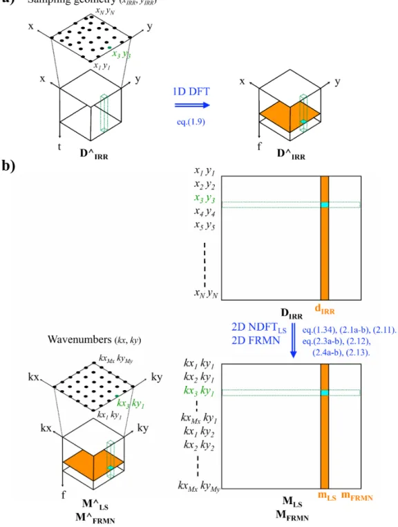
Figure 1: Schematic representation of the first step of the LS Fourier reconstruction. (a)
The original 3D data volume D∧
IRR(in time-space coordinates) is transformed in the temporal
frequency domain. The dots indicate the actual spatial positions (xIRR, yIRR) of the traces.
(b) The 3D data volume D∧
IRR(in frequency-space coordinates) is arranged in lexicographical
order into a 2D matrix DIRR. Each column of DIRR, that is a vector dIRR, corresponds to
a frequency slice of D∧
IRR. Each row of DIRRcorresponds to a data trace of D∧IRR. The 3D
Fourier spectrum M∧
LS (or M
∧
FRMN) can be estimated from the 3D data using a 2D NDFTLS
(or 2D FRMN), as discuss in the text. MLS (or MFRMN) is the 3D Fourier volume M∧LS (or
M∧
FRMN ) arranged in a 2D matrix. Each column of MLS(or MFRMN), that is a vector mLS
(or mFRMN), corresponds to a frequency slice of M∧LS (or M
∧
FRMN ). Each row of MLS (or
MFRMN) corresponds to a temporal frequency spectrum in M∧LS (or M
∧
FRMN ). Note that
the Fourier elements of M∧
LS (or M
∧
2.1. LS FOURIER RECONSTRUCTION: A TWO-STEP METHOD 38
Equation (2.1a) can be rewritten as:
mLS= (GHWG)
−1
∆kx∆kymNDFT (2.1b)
where the column-vector mNDFT is a temporal frequency slice of the the 3D
NDFT spectrum (M∧
NDFT) of the 3D irregularly sample data set; mNDFT is
equal to the GHWd
IRR matrix-vector product in equation (2.1a), apart from
the constant factor ∆kx∆ky. The inverted Gram matrix (GHWG)−1 acts as
a deconvolution operator for the spectral leakage, as discussed in the Chapter 1. However, the structure of the forward operator G (and thus the structure
of GHWG is usually ill conditioned. Due to small singular values, an ill
con-ditioned problem is effectively underdetermined (i.e., numerical rank deficient) (Hansen (1998)). For a stable inversion and to retrieve an unique and noise-free LS Fourier spectrum, additional constraints or a-priori information on model parameters must be incorporated in the LS inversion. Unfortunately, there is no a-priori knowledge in the Bayesian sense regarding either the model param-eters and the noise distribution for this type of inverse problem (Duijndam et
al.(1999)). Therefore, to overcome the combination of noise (spectral leakage)
and ill conditioning, FRMN adopts the simple strategy of adding a restriction
on the Euclidean model norm to the cost function of the 2D NDFTLS (equation
(1.33)) (Hindriks and Duijndam (2000)):
JFRMN= ∥W−
1
2 (dIRR−Gm) ∥2
2+λ∥m∥22. (2.2)
The damped least-squares (DLS) cost function of equation (2.2) is also known as the zero-order Tikhonow cost function (Aster et al. (2005)). The damping (or tuning) parameter λ is a positive constant that acts as a stabilization term to balance the influences of the LS data misfit (the first term of equation (2.2)) and the quadratic penalty term (the second term of equation (2.2)). Because the cost function into equation (2.2) is strictly convex, the unique minimum given is by:
mFRMN=G−gF RM NdIRR= (GHWG + λI)
−1
GHWdIRR. (2.3a)
The subscript FRMN is used to remark that minimum energy constraints are
used in the estimation process and G−gFRMN = (GHWG + λI)
−1
GHW is the
(weighted) DLS generalized inverse of G. Equation (2.3a) can be rewritten as:
mFRMN= (GHWG + λI)
−1
∆kx∆kymNDFT (2.3b)
where the term λ can be viewed as a pre-whitening term in the deconvolution. In equations (2.3a) and (2.3b), instead of using a damped least-squares scheme,
the inverse of the Gram matrix GHWGcan be computed by truncated singular
value decomposition (TSVD):
CHAPTER 2. LEAST-SQUARES FOURIER RECONSTRUCTION OF SEISMIC DATA
or
mFRMN= (GHWG)
†
∆kx∆kymNDFT (2.4b)
where † denotes the Moore-Penrose pseudo-inverse (Aster et al. (2005)) and,
in this case, G−gFRMN= (GHWG)
†GHW is the TSVD generalized inverse of G.
The equivalence between employing a damping factor λ as in equations (2.3a) and (2.3b) and the application of a TSVD as in equations (2.4a) and (2.4b) can be easily demonstrated via filter factor analysis (Aster et al. (2005)).
Least-squares or minimum norm formulation
The least-squares estimator in equations (2.1a) or (2.1b) cannot be applied
to an underdetermined problem in which the number (NIRR) of traces with
coordinates (xIRR, yIRR) of the irregularly sampled grid is less than the number
(M = (Mx×My)) of estimated Fourier coefficients (kx, ky). Conversely, for a
damped least-squares estimate (equations (2.3a) or (2.3b)) the following identity from Snieder and Trampert (1999):
(GHWGW+λI) −1 GHW = 1 λG H W(I + GW 1 λG H W) −1 =GHW(GWGHW +λI) −1 (2.5) with GW =W− 1
2G, shows that when damping is used, the damped least-squares
solution (the left-hand side of equation (2.5)) and the damped version of the minimum-length solution (the right-hand side of equation (2.5)) are identical.
For NIRR <M, the damped minimum-length solution is more efficient than the
damped least-squares solution because the matrix GWGHW, of size NIRR×NIRR,
is smaller than the matrix GH
WGW, of size M × M.
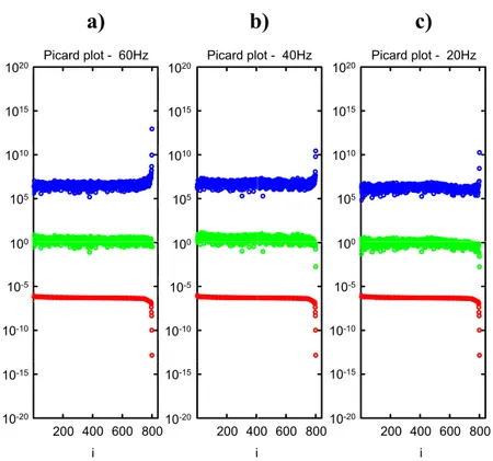
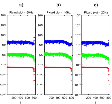
Ill conditioning and stability: the discrete Picard condition
In the 2D NDFTLS(equations (2.1a) and (2.1b)) the ill conditioned nature of the
forward operator G is strictly related to the irregularity in the spatial sampling,
and as sampling becomes more non-uniform, the condition number1 of G (and
thus the condition number of GHWG) increases. SVD analysis is particularity
useful to determinate how the combination of noise (the spectral leakage in the NDFT) and the ill conditioning affect the stability of the LS inversion. In
particular, using the SVD representation of the Gram matrix GHWG, equation
(2.1b) can be written as:
mFRMN=∆kx∆ky(VS−1UH)mNDFT=∆kx∆ky∑
i
uH
(i)mNDFT(i)
S(i,i) v(i) (2.6)
1The condition number of a matrix is defined as the ratio between its largest and smallest