ASASSN-15nx: A Luminous Type II Supernova with a “Perfect” Linear Decline

10.3847/1538-4357/aacb35

DOI

http://hdl.handle.net/20.500.12386/27523

Handle

THE ASTROPHYSICAL JOURNAL

Journal

862

ASASSN-15nx: A Luminous Type II Supernova with a

“Perfect” Linear Decline

Subhash Bose1,17 , Subo Dong1,17 , C. S. Kochanek2,3 , Andrea Pastorello4, Boaz Katz5, David Bersier6 , Jennifer E. Andrews7, J. L. Prieto8,9 , K. Z. Stanek2,3, B. J. Shappee10, Nathan Smith7, Juna Kollmeier11 , Stefano Benetti4,

E. Cappellaro4 , Ping Chen1, N. Elias-Rosa4, Peter Milne7 , Antonia Morales-Garoffolo12, Leonardo Tartaglia13 , L. Tomasella4, Christopher Bilinski7, Joseph Brimacombe14, Stephan Frank2, T. W.-S. Holoien11, Charles D. Kilpatrick15 ,

Seiichiro Kiyota16, Barry F. Madore11 , and Jeffrey A. Rich11 1

Kavli Institute for Astronomy and Astrophysics, Peking University, Yi He Yuan Road 5, Hai Dian District, Beijing 100871, People’s Republic of China

2

Department of Astronomy, The Ohio State University, 140 W. 18th Avenue, Columbus, OH 43210, USA

3

Center for Cosmology and AstroParticle Physics(CCAPP), The Ohio State University, 191 W. Woodruff Avenue, Columbus, OH 43210, USA

4

INAF-Osservatorio Astronomico di Padova, Vicolo dell’Osservatorio 5, I-35122 Padova, Italy

5

Weizmann Institute of Science, Rehovot, Israel

6

Astrophysics Research Institute, Liverpool Science Park, 146 Brownlow Hill, Liverpool L3 5RF, UK

7

Steward Observatory, University of Arizona, Tucson, AZ 85721, USA

8

Núcleo de Astronomía de la Facultad de Ingeniería y Ciencias, Universidad Diego Portales, Av. Ejército 441, Santiago, Chile

9

Millennium Institute of Astrophysics, Santiago, Chile

10

Institute for Astronomy, University of Hawaii, 2680 Woodlawn Drive, Honolulu, HI 96822, USA

11_{Carnegie Observatories, 813 Santa Barbara Street, Pasadena, CA 91101, USA} 12

Department of Applied Physics, University of Cádiz, Campus of Puerto Real, E-11510 Cádiz, Spain

13

Department of Astronomy and The Oskar Klein Centre, AlbaNova University Center, Stockholm University, SE-106 91 Stockholm, Sweden

14

Coral Towers Observatory, Cairns, Queensland 4870, Australia

15

Department of Astronomy and Astrophysics, University of California, Santa Cruz, CA 95064, USA

16

Variable Stars Observers League in Japan(VSOLJ), 7-1 Kitahatsutomi, Kamagaya 273-0126, Japan Received 2018 March 31; revised 2018 June 4; accepted 2018 June 5; published 2018 July 27

Abstract

We report a luminous Type II supernova, ASASSN-15nx, with a peak luminosity of MV = -20 mag that is between those of typical core-collapse supernovae and super-luminous supernovae. The post-peak optical light curves show a long, linear decline with a steep slope of 2.5 mag(100 day)−1(i.e., an exponential decline in flux) through the end of observations at phase »260 day. In contrast, the light curves of hydrogen-rich supernovae (SNe II-P/L) always show breaks in their light curves at phase ∼100 day, before settling onto 56

Co radioactive decay tails with a decline rate of about 1 mag(100 day)−1. The spectra of ASASSN-15nx do not exhibit the narrow emission-line features characteristic of Type IIn SNe, which can have a wide variety of light-curve shapes usually attributed to strong interactions with a dense circumstellar medium (CSM). ASASSN-15nx has a number of spectroscopic peculiarities, including a relatively weak and triangular-shaped Hα emission profile with no absorption component. The physical origin of these peculiarities is unclear, but the long and linear post-peak light curve without a break suggests a single dominant powering mechanism. Decay of a large amount of 56Ni (MNi=1.6±0.2 M) can power the light curve of ASASSN-15nx, and the steep light-curve slope requires

substantialγ-ray escape from the ejecta, which is possible given a low-mass hydrogen envelope for the progenitor. Another possibility is strong CSM interactions powering the light curve, but the CSM needs to be sculpted to produce the unique light-curve shape and avoid producing SN IIn-like narrow emission lines.

Key words: supernovae: general– supernovae: individual (ASASSN-15nx)

1. Introduction

Core-collapse supernovae(CCSNe) are generally believed to originate from the collapse of massive stars with zero age main sequence (ZAMS) masses MZAMS8M. The properties of

the resulting transient depend strongly on the mass and composition of the star at death. In particular, Type II supernovae(SNe) represent the broad subclass of CCSNe that have retained a substantial amount of hydrogen envelope at the time of explosion. Their spectra show characteristic prominent hydrogen Balmer lines with P-Cygni profiles, while the other subclasses of CCSNe (Ib and Ic) are characterized by the absence of hydrogen in their spectra.

Traditionally, these hydrogen-rich SNe are classified into two major subclasses, Type II-P and II-L(Barbon et al.1979; Filippenko 1997), based on their light curve shapes in the

photospheric phase. In this classification scheme, the light curve of a SN II-P has a plateau with almost constant brightness for a period of nearly 100 days, whereas the light curve of an SN II-L declines linearly in magnitude after its peak. Various attempts have been made to refine the classifying criteria of these two subclass (see, e.g., Arcavi et al. 2012; Faran et al.2014). However, with more detections of SNe-II, it

has been realized that SN II light curves are too diverse to perfectly divide into “plateau” or “linear” shapes (e.g., Bose et al.2016; Holoien et al.2016b; Valenti et al.2016), and that

the distribution of light-curve shapes may be continuous rather than bimodal(Anderson et al.2014). A continuous distribution

of light curve decline rates suggests a continuum in the ejecta parameters controlling the light-curve shape(e.g., the progeni-tor density profile according to Nakar et al.2016). Hereafter,

we would refer them as a unified subclass: Type II-P/L SNe. At the end of the photospheric phase, there is a sudden change in the light-curve shape of SN II-P/L to an exponential © 2018. The American Astronomical Society. All rights reserved.

17_{Corresponding authors: Subo Dong(dongsubo@pku.edu.cn), Subhash Bose}

γ-ray photons released from the nuclear decay. For SNe II-P/L, the ejecta mass is typically large enough to efficiently absorb and thermalize the decay energy, leading to a luminosity decline rate close to the nuclear decay rate. With the end of the recombination-dominated photo-spheric phase and the onset of the radioactive tail phase, there is a sharp transition in the optical light curve. This transition phase is always seen for all SN II-P/L with well-covered late-time light curves(Anderson et al. 2014).

CCSNe originate from a wide range of progenitors, and their observed properties also show great diversity. The peak absolute magnitude of Type Ib/c and Type II-P/L SNe typically lie within a broad range of MV∼−14 to −18.5 mag

(Li et al. 2011b). In the last decade, we have also seen the

emergence of what may be a new class of events: super-luminous supernovae(SLSNe) (e.g., Quimby et al.2007; Smith et al. 2007; Dong et al. 2016; Bose et al. 2018). They are

10–100 times more luminous than typical CCSNe and peak at MV<−21 mag. Their explosion physics and powering

mechanisms are not yet understood, though many hypothesize that their progenitors may be stars more massive than those of common CCSNe(Gal-Yam2012). It is an open question as to

whether there is a gap in the SN luminosity function between those of common SNe and the SLSNe(Arcavi et al.2016); the

answer to this question may indicate whether the progenitor masses of SLSNe are just an extension of the normal SNe. Only a few SNe have been discovered with intermediate luminosity (e.g., PTF10iam with MV,peak≈−20 mag; Arcavi

et al.2016).

Here, we report the latest addition to this rare group of events with luminosities between those of typical CCSNe and SLSNe: ASASSN-15nx. We present the discovery and follow-up observations of this Type II SN to late time, and wefind that, unlike any known SN II-P/L, its late-time light curves do not show the transition to a nuclear decay tail.

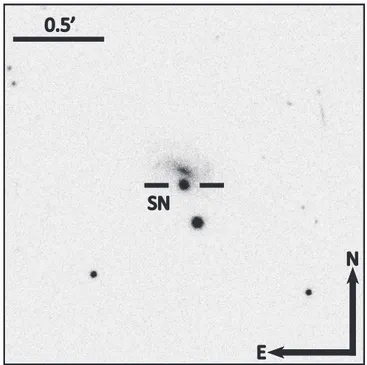
ASASSN-15nx was discovered (Kiyota et al. 2015; Holoien et al. 2017a) in the galaxy GALEXASCJ044353.08-094205.8

(see Figure1for an image of the supernova and its host galaxy) on 2016 August 8 during the ongoing All-sky Automated Survey for SuperNovae (ASAS-SN; Shappee et al. 2014), using the

quadruple 14 cm “Brutus” telescope at the LCO facility on Haleakala, Hawaii. The ASAS-SN survey regularly scans the entire visible sky for bright supernovae and other extragalactic transients down to V∼17 mag, and the ASAS-SN discoveries are minimally biased by host galaxy properties (Holoien et al.

2017a). Nearly 100% of the ASAS-SN supernovae also have

spectroscopic classifications (Holoien et al.2017a,2017b,2017c).

As a result, the ASAS-SN survey provides an unprecedented, spectroscopically complete, host-unbiased sample from an untargeted survey to study supernova statistics. It has also found a range of unusual transients that likely would have been missed in many other surveys (e.g., Dong et al. 2016; Holoien et al.

2016a; Bose et al. 2018). ASASSN-15nx is located at α=

04h43m53 19 d = -09 42 11. 22, which is offset by 0 9 E and ¢ 

5 1 S from the center of the z=0.02823 (see Section3; DL=

127.5 Mpc) host galaxy GALEXASCJ044353.08-094205.8 (or PGC 987599; a = 04 43 53. 13h m s _{, d = -09 42 06. 1 ¢  ). The}

off-set from the host center is 3.2kpc.

The first detection of ASASSN-15nx was on 2015 July 16.42 UTC (JD 2457219.92). We adopt 2015 July 15.60 (JD2457219.10±2.00) as the explosion epoch based on fitting the early rising of the light curve with the analytical model from Rabinak & Waxman(2011). We used this as the

reference epoch throughout the paper(see Section3for further details on the method of constraining the explosion epoch). The object was classified by Elias-Rosa et al. (2015) as a Type II

supernova, based on the presence of an Hα emission line. It was further noted that the Hα emission had a peculiar, triangular profile, along with metal lines that appeared to be unusually strong.

We provide brief descriptions of the data collected for ASASSN-15nx in Section 2. We discuss how we estimate explosion epoch, distance, and extinction in Section 3. In Sections 4 and 5, we perform detailed photometric and spectroscopic characterization of the SN. We also identify various peculiarities, which are summarized in Section 6. Finally, in Section 7, we discuss various scenarios that may explain the unique properties of ASASSN-15nx.

2. Data

We initiated multi-band photometric and spectroscopic observations soon after the discovery(+25 day) and continued the observations of ASASSN-15nx until +262 day. Photo-metric data were obtained from the ASAS-SN quadruple 14 cm “Brutus” telescope, the Las Cumbres Observatory 1.0 m telescope network (Brown et al. 2013), the 1.8 m Copernico,

0.8 m TJO, 2.4 m MDM, 2.6 m NOT, 2.0 m Liverpool telescope, 6.5 m Magellan Baade, and 0.6 m Super-Lotis telescopes. The data were obtained in the Johnson–Cousins BVRI and SDSS gri broadband filters. The images were reduced using standardIRAF tasks, and PSF photometry was

Figure 1. 2′×2′ g′-band image from the 2.6 m Nordic Optical Telescope showing ASASSN-15nx and its host GALEXASCJ044353.08-094205.8.

performed using the DAOPHOT package. The PSF radius and background extraction region were adjusted according to the FWHM of the image. Photometric calibrations are done using APASS (DR9; Henden et al. 2016) standards available in the

field of observation. The R- and I-band standards were converted from Sloan gri magnitudes using the transformation relation given by Lupton et al.(2005). The photometric data of

ASASSN-15nx are reported in Table1.

Medium- to low-resolution spectroscopic observations were made using AFOSC mounted on the 1.8 m Copernico, the Boller & Chivens Spectrograph on the 2.3 m Bok, ALFOSC on the 2.6 m NOT, the Blue Channel spectrograph on the 6.5 m MMT, IMACS and MagE on the 6.5 m Magellan Baade telescope, the Boller & Chivens Spectrograph on the 2.5 m Irénée du Pont, and MODS on the LBT with an effective diameter of 11.9 m. All observations were performed in long-slit mode and spectroscopic reductions were done using standard IRAF tasks. The medium-resolution spectra from MODS were reduced using the modsIDL pipeline. The LBT MODS observation on 2016 January 2.20 was also used to estimate the redshift of the host galaxy(see Section3), with the

slit aligned to cross both the host nucleus and the SN. The spectroscopic observations are summarized in Table 2.

3. Explosion Epoch, Distance, and Extinction The first confirmed detection of ASASSN-15nx was on JD2457219.92 (2015 July 16.42 UTC), and the last non-detection was about 15 days earlier on JD2457204.94 with a limiting magnitude of V=17.1 mag. This 15 day gap prevents us from rigorously constraining the explosion epoch directly from observations. However, subsequent observations after the initial detection captured the early rise of the light curve. We modeled these data following Rabinak & Waxman (2011),

which is strictly applicable within a couple of weeks after explosion. First, we construct the blackbody SED using the temperature and radius from the Rabinak & Waxman (2011)

prescription for a red-supergiant progenitor. The SED is then redshifted and corrected for extinction. The model SED evolution can be represented as

l l = -l -⎡ ⎣⎢

(

)

where t0is the explosion epoch, A and B are free parameters,

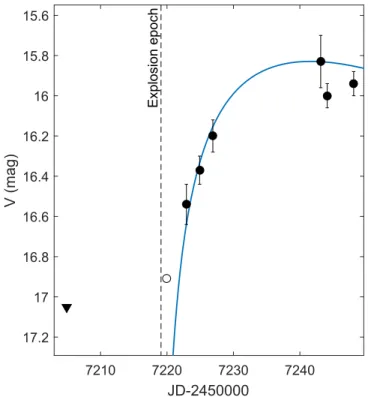
and λ and t have the usual meanings of wavelength and time. The resulting SED evolution is then convolved with the V-band filter response to obtain the model light curve. The fit to the early V-band observations is shown in Figure2. Even though the nominal detection significance of the first detection is high, the quality of the image is poor and we exclude it from the model fitting. The data for the subsequent three epochs are cleaner and provide most of the model constraints, leading to an estimated explosion epoch of JD2457219.10±2.00 (2015 July 15.60 UTC), which is ∼0.8 days prior to our first detection. We adopt this as the reference epoch throughout the paper. The estimated rise time from explosion to V-band peak is then ≈22 days.

The host galaxy of ASASSN-15nx does not have any archival redshift or distance estimate. We took a medium-resolution LBT/ MODS spectrum with the slit crossing the nucleus of the host

galaxy on 165.9 day. The spectrum revealed narrow HIlines(see Figure3), with Hα being the most prominent feature at 6748.1 Å,

corresponding to a host redshift of z=0.02823. The weaker Hβ line was also detected at 4999.4Å, corresponding to a z= 0.02840. These two values are consistent and we adopt z= 0.02823 from the strong Hα line. This redshift is also consistent with that inferred from the faint, narrow Hα emission visible on top of the broad Hα P-Cygni profile in four late SN spectra taken between days 166 and 262. The corresponding luminosity distance and distance modulus are DL=127.5±1.7 Mpc and

DM= 35.53±0.03 mag, assuming a flat cosmology withH0=

-

-67.7 km s Mpc1 1_andΩ

m=0.308 (Planck Collaboration et al.

2016).

In the 165.9 day SN spectrum, we detect Galactic NaID absorption at 5893Å. We do not detect any NaID absorption feature at the redshift of the host, which indicates that the host extinction is likely negligible. Therefore, we adopt a total line-of-sight reddening of E B( -V)=0.07 mag (Schlafly & Finkbeiner 2011), entirely due to the Milky Way, which

translates into AV=0.22 mag, assuming RV=3.1 (Cardelli

et al.1989).

4. Light Curve

4.1. Light Curve Evolution and Comparison

The most unique feature of ASASSN-15nx is its long-lasting, fast-declining linear light curve during the entire phase of evolution following the maximum, as shown in Figure 4. Post-maximum linear decline at a constant rate is observed in all photometric bands, excepting only the B-band, which has a steeper slope for50 day. This exceptionally long and nearly “perfectly” continuous linear decline in most optical bands has

Figure 2.Modeling of the early V-band light light curve of ASASSN-15nx, to constrain the explosion epoch. Thefilled triangle shows the last ASAS-SN non-detection. The open circle represents thefirst confirmed detection of the SN, but with uncertain photometry. The estimated explosion epoch 0.8 days prior to thefirst detection is indicated by the dashed line.

not been seen in any other SNe observed to date. The rest-frame light curve decline rates are 2.48±0.03, 2.53±0.08, 2.65±0.04, 2.82±0.25, 2.47±0.10, 2.51±0.09 mag (100 day)−1 _{in the V, R, I, g, r, and i bands, respectively.}

The B band light curve slope is 5.28±0.28 mag (100 day)−1 for<52 day and 2.46±0.07 mag (100 day)−1 afterward.

We compare the absolute V-band (MV) light curve of

ASASSN-15nx with those for 116 Type II-P/L SNe from Anderson et al.(2014) in Figure5. The comparison shows that the SN clearly stands out from the sample in terms of both absolute magnitude and the nearly perfect, long linear decline of the light curve. The V-band maximum absolute magnitude observed for ASASSN-15nx is−19.92±0.06mag, making it ∼2.8 mag brighter at +50 day than typical Type II-P/L SNe in the sample.

We further compare ASASSN-15nx with a sample of well-studied Type II-P/L SNe in Figure 6. The slope of the SN is comparable to the slope during the photospheric phase of SNe 2014G (2.55 mag (100 day)−1), 2013by (2.01 mag (100 day)−1_{), and 2000dc (2.56 mag (100 day)}−1_{) (Bose et al.}

2016), all of which are fast-declining Type II SNe, also known

as SNe II-L. All Type II SNe light curves in the comparison sample show distinct photospheric and radioactive tail phases, with a transition near 80–120 days. For qualitative comparison, we also include the absolute R-band light curve of PTF10iam (Arcavi et al. 2016) and the g-band light curve of

ASASSN-15no (Benetti et al. 2018) in Figure 6. PTF10iam had an absolute magnitude similar to ASASSN-15nx(∼−20 mag) and a somewhat slower decline rate of 2.32 mag (100 day)−1. PTF10iam is characterized as a luminous and rapidly rising SN II. ASASSN-15nx may have risen equally rapidly, but there is insufficient pre-peak data to be certain. PTF10iam was only observed for ∼90 days, which is a typical timescale for the photospheric phase to have a nearly constant decline rate, so it is not possible to determine whether it had a unique, long-lived linear decline similar to ASASSN-15nx. SN 1979C, SN 1998S, and ASASSN-15no had maximum brightnesses close to, albeit a few tenths of a mag fainter than, that of ASASSN-15nx; they also have late-time light curve decline rates comparable to ASASSN-15nx. However, the light curves of SN 1979C, SN 1998S, and ASASSN-15no show prominent breaks near ∼90 days, so they do not exhibit the most distinguishing feature: the long and continuous linear decline of ASASSN-15nx.

The characteristic radioactive tail phase of normal SNe II (150 days), powered by Co56 _to 56_{Fe decay, has a decline}

slope of ∼0.98mag (100 day)−1 when the γ-ray photons are fully trapped. During this phase, most SNeII in Figure6show a decline rate consistent with almost full trapping of the γ-rays. The light curve of ASASSN-15nx is significantly steeper and continued to decline with a constant slope after the early peak. In comparison, the tail of the light curve of the prototypical Type Ia SN 2011fe(Munari et al.2013), which is also powered by Co56

to 56Fe_{radioactive decay, has a slope comparable to} ASASSN-15nx. The substantially lower γ-ray optical depth in SNe Ia increases the fraction of escapingγ-ray photons and makes the light curve steeper than typical SNe II. The similarity in light

Figure 3.Spectrum for the host nucleus with narrow Hα and Hβ lines at a redshift z=0.02823.

Figure 4.Photometric light curves in the Johnson–Cousins BVRI and SDSS gri bands. The light curves are vertically shifted for clarity.

Figure 5.Absolute V-band light curve of ASASSN-15nx(red), compared with the sample of Type II SNe presented by Anderson et al.(2014).

curve shapes between SNe Ia and luminous SNe IIL, such as SN1979C, has been discussed before(Doggett & Branch1985; Wheeler et al. 1987; Young & Branch 1989), pointing to the

possibility that luminous SN IIL might also be powered by the decay of a large amount of 56Ni, like SNe Ia. We explore this possibility for ASASSN-15nx in Sections4.2and7.1.

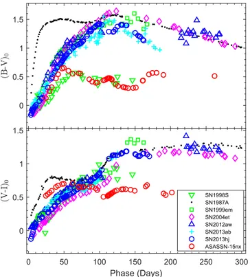
In Figure7, we present the extinction-corrected(B−V )0and

(V−I)0 color evolution of ASASSN-15nx, as compared with

several SNe IIP/L and the Type IIL/n SN1998S. For ASASSN-15nx, the magnitudes are loosely interpolated to match corresponding photometric epochs for each pair of bands; this also serves to reduce the randomfluctuations from internal uncertainties in the photometry. For t<50 day, ASASSN-15nx continues to become redder, following a trend similar to other SNe II. After +50 day, however, ASASSN-15nx shows very little change in color, with mean values (B−V )0=0.450±

0.016 and(V−I)0=0.598±0.009 mag. By contrast, a typical

SNe IIP/L continues to evolve to substantially redder colors. However, SN IIL/n SN1998S shows a color evolution similar

to ASASSN-15nx in terms of the mean colors and the absence of evolution after∼60 days.

We fit blackbody models to the extinction-corrected B-, V- and I-band magnitudes. Figure 8 shows the resulting evolution of the effective temperature and radius. The radius initially increases until+50 days, where the photospheric phase ends and the ejecta becomes optically thin. During this phase, the temperature shows a steady decline as the ejecta cools down with expansion. The best-fit effective temperature then starts to rise until ∼135 days, before again beginning a slow decline. This blackbody temperature evolution is unlike that of normal SNe, where usually we simply see monotonic declines (e.g., Bose et al.2013,2015b).

4.2. Bolometric Light Curve and 56Ni_Mass

In Figure9, we compare the pseudo-bolometric(3335–8750 Å) light curves of ASASSN-15nx to a sample of well-studied SNe II. The pseudo-bolometric luminosities for all SNe in the sample are constructed following the method described in Bose et al.(2013).

Figure 6.Absolute V-band light curve of ASASSN-15nx, as compared to other Type II SNe and the Type Ia SN 2011fe. The exponential decline of a light curve following the radioactive decay law for56Co 56Fe_{is shown with a black dashed line. A best-fit straight line (yellow dashed) is shown on top of the ASASSN-15nx} light curve, to emphasize the linearity of decline. On the bottom left side, pairs of dashed lines in gray and green represent the slope range for the Type II-P and II-L SNe templates, as given by Faran et al.(2014). The adopted explosion time in JD-2400,000, distance in Mpc,E B( -V)in mag, and the references for observed V-band magnitude, respectively, are : SN 1979C—43970.5, 16.0, 0.31; Barbon et al. (1982b), de Vaucouleurs et al. (1981); SN 1980K—44540.5, 5.5, 0.30; Barbon

et al.(1982a), NED database; SN 1987A—46849.8, 0.05, 0.16; Hamuy & Suntzeff (1990); SN 1999em—51475.6, 11.7, 0.10; Leonard et al. (2002); Elmhamdi et al.

(2003); SN 2000dc—51762.4, 49.0, 0.07; Faran et al. (2014), NED database; SN 2004et—53270.5, 5.4, 0.41; Sahu et al. (2006); SN 2009bw—54916.5, 20.2, 0.31;

Inserra et al.(2012); SN 2012A—55933.5, 9.8, 0.04; Tomasella et al. (2013); SN 2012aw—56002.6, 9.9, 0.07; Bose et al. (2013); SN 2013ab—56340.0, 24.0, 0.04;

Bose et al.(2015b); SN 2013by—56404.0, 14.8, 0.19; Valenti et al. (2015); SN 2013ej—56497.3, 9.6, 0.06; Bose et al. (2015a); SN 2013hj—56637.0, 28.2,

0.10; Bose et al.(2016); SN 2014G— 56669.7, 24.4, 0.25; Bose et al. (2016); PTF10iam— 55342.7, 453.35, 0.19; Arcavi et al. (2016); SN 2011fe—55797.2, 6.79,

The light curve decline rate for ASASSN-15nx is 1.05 dex (100 day)−1_{, which is ∼3 times faster than that expected for a}

light curve powered by the radioactive decay of 56Co_to 56_Fe.

Next, we modeled the blackbody bolometric luminosity, using a pure radioactive 56Ni56Co  56Fe _{decay model. The two} free model parameters are the 56Ni _{mass M}

Ni and the γ-ray

trapping parameter t_0γ, which defines the evolution of the γ-ray optical depth as t ~g t02g t2. While all the positron kinetic energy

from56Co_{decay is trapped, only -}

-g

[1 exp( t0 t )]

2 2 _{fraction of}

the γ-ray decay energy is trapped in the envelope (see the discussions of this approximation in, e.g., Clocchiatti & Wheeler

1997; Chatzopoulos et al. 2012). As shown in the top panel of

Figure10, wefind a reasonable fit for MNi=1.6±0.2Mand a

γ-ray trapping factor t0γ=73±7 days. Although the overall light

curve is matched well by the model, there are some noticeable deviations at both early(<25 days) and late (∼200 days) times. Even if the light curve is entirely powered by the radioactive decay, this simple model is not expected to fully capture the light-curve evolution at early phases when the ejecta is optically thick and diffusion is important. The deviation at late time might reflect

Figure 7.Color evolution of ASASSN-15nx, as compared to the well-studied Type II SNe 1987A, 1999em, 2004et, 2012aw, 2013ab, and 2014hj, and also the Type IIL/n SN 1998S. The references for the data are same as in Figure6.

Figure 8.Temporal evolution of the blackbody temperature(blue, left scale) and radius(red, right scale) of ASASSN-15nx.

Figure 9. UBVRI pseudo-bolometric light-curve of ASASSN-15nx, as compared to other well-studied SNe. Light curves, including UV contributions, are also shown for SNe 2012aw, 2013ab, and 2014G(labeled as UVO). The adopted distances, reddenings, and explosion times are the same as in Figure6. The slope of a light curve powered by the radioactive decay of56Co56Fe_is shown with the dashed line.

Figure 10.Radioactive decay models of the bolometric light curve(top panel) and the time-weighted integrated radiated energy (bottom panel) of ASASSN-15nx.

inaccuracies in either the physical assumptions of the simple radioactive decay model or the blackbody model used in deriving the bolometric light curve.

To gain more insight into the powering source, we also used the time-weighted integrated luminosity method to model the light curve (Katz et al. 2013; Nakar et al. 2016; Wygoda et al. 2017). The results are shown in the bottom panel of

Figure 10. By comparing time-weighted integrated luminosity with a radioactive decay model during the post-photospheric phase, we can verify the powering source of the entire light curve. Katz et al. 2013 showed that the time-weighted integrated luminosity(

ò

0 can also be used to put an

additional constraint on the 56Ni _{mass during the} post-photospheric phase—provided the light curve is solely powered by radioactive decay, as in SNe Ia. For this purpose, early time estimates of the luminosity are required, so we extrapolated the temperature into the pre-peak phases and scaled the SED to the V-band flux at fixed temperature. The blackbody luminosity is listed in Table3. The uncertainty introduced by the extrapolation will eventually become smaller, at larger values of t, due to the time weighting of the integral. The comparison of the integrated time-weighted luminosity shows that the total energy budget of ASASSN-15nx is consistent with almost fully radioactive decay energy, which raises the possibility that it is the dominant powering source of the light curve.

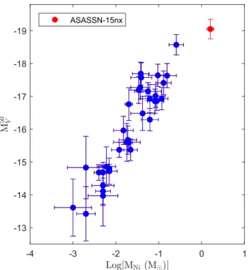
In Figure11, we show the correlation between the56Ni_mass and the V-band luminosity MV

50

at t=50 days for the 34 Type II SNe from Hamuy(2003) and Spiro et al. (2014), along with

ASASSN-15nx. As one would expect, 56Ni _{mass increases} with luminosity, but with considerable scatter in the correlation (see Pejcha & Prieto 2015). ASASSN-15nx is consistent with

an extrapolation of this correlation, while it clearly stands out at the higher extreme end of the luminosity distributions.

The blackbody model may not always be a good approx-imation, especially in the optical thin phases. We also constructed the bolometric light curve using bolometric corrections derived empirically from other well-observed Type II SNe. The correction factor is calibrated as a function of broadband color. We adopt the bolometric correction from Bersten & Hamuy(2009) based on the (B−V ) color. Because

B-band data are not available during the pre-peak phases, the (B−V ) color is linearly extrapolated from the color curve for t<50 days. By modeling this bolometric light curve, we estimate MNi=1.3±0.2 M and t0g=7110 days. This

value of nickel mass is consistently within ∼20% of that estimated with our earlier model, and theγ-ray trapping factor is also similar. We caution that the bolometric luminosities used in this method may also be inaccurate for an SN like ASASSN-15nx, whose light curve, color, and spectroscopic evolution are significantly different from generic SNe II.

5. Optical Spectra 5.1. Key Spectral Features

The spectroscopic evolution of ASASSN-15nx from t=53 to 262 days is presented in Figure 12. One striking feature is the Hα emission profile, which has an unusual triangular shape in the earliest spectra at t=53 days. We further discuss the Hα profile and its evolution in Sections 5.2 and 5.3. Forbidden[CaII] (ll 7291, 7324) emission, which usually is not visible until the early nebular phase (120 days), can be seen throughout our observing campaign. The CaIImultiplets (ll 8498, 8542, and 8662) are not detected at t=53.3 days, though the SNR in the relevant part of the spectrum is relatively low, while they are clearly visible at t=87.4 days, which is typical of SNe IIP/L. OI emission near 7780Å is another prominent feature in the 53 day spectra and is present throughout the spectral evolution. The strong OI emission feature appears unusually early for a Type II SN. Interestingly, the OIline has a doubly peaked profile in the 53 day spectra, which evolves into a singly peaked profile by 96.7 days and is no longer present in all subsequent spectra. The origin of the redder component of the double-peaked profile is not clear (as indicated by a question mark in Figure12). The overall spectral

appearance and the early presence of [CaII] and strong OI features at day 53 make the spectrum appear much more evolved than typical SNe IIP/L at a similar phase. Another noticeable feature in all the spectra is the apparent continuum break near 5500Å. The continuum level on the bluer side is about 25% higher than on the red side(see further discussions in the context of SYNOW modeling below and also in Section7.2). The evolution of the prominent metallic lines of

FeII(ll 4924, 5018, 5169) and NaID (5893 Å) is typical of SNe II.

We usedSYNOW18(Fisher et al. 1997, 1999; Branch et al.

2002) to model the spectra and identify features. In order to

mimic the continuum break, we multiply the model spectrum with a Gaussian convolved step function whose amplitude and width are tuned to fit the observed spectrum. This modifier function is shown in the top panel of Figure13, where the blue continuum beyond 5500Å is ∼25% higher than the red, with a 150Å width for the convolving Gaussian function.

Figure 11. Absolute V-band magnitude at t=50 days as a function of the estimated56Ni_{mass for the SNe II sample, from Hamuy(2003) and Spiro et al.} (2014). ASASSN-15nx, shown with a red dot, lies on the extrapolation of the

correlation to higher masses and luminosities.

18

The set of atomic species used to generate the synthetic spectrum are HI, HeI, OI, FeII, TiII, ScII, CaII, BaII, NaI, and SiII. As noted above, ASASSN-15nx exhibits an unusual, triangular Hα emission with a weak absorption feature on the blue side that is not consistent with a P-Cygni profile. The Hβ profile is also unusually broad and extended, which SYNOW could not reproduce with a single Hβ component using any combination of expansion velocity and optical depth profile. Therefore, the Hα and Hβ line region have been masked in the synthetic spectrum. Apart from the nebular-like emission features of CaIIand OI, for which SYNOW is not applicable, many of the spectral features are reasonably well-reproduced— except for the ScIIfeatures at 4274 and 4670Å.

In the SYNOW model, the absorption feature near 6300Å, which appears to form the absorption component of the P-Cygni profile associated with Hα, is reproduced by SiII (6355 Å). The SiII velocity is same as the photospheric

velocity(~3.3´10 km s3 -1_{) found for the other metal lines,}

affirming the line identification and suggesting that there is little or no absorption component associated with Hα.

5.2. Comparison of Spectra

We compare spectra of ASASSN-15nx to other Type II SNe at three different phases (53.0 days, 121.0 days, 262.0 days), as shown in Figures14–16. Figure14shows the comparisons of the 53.0 day spectrum. Apart from the Hα profile, the spectral features broadly resemble most of the other SNeII spectra in the comparison sample. The Hα profile of ASASSN-15nx is significantly weaker and unusually triangular in shape, compared to other SNe II. For instance, normal SNeII at t≈53 days have a mean Hα equivalent width of ∼157 Å (Gutiérrez et al. 2017),

whereas we find a significantly lower value of ∼117 Å for ASASSN-15nx and it stays systematically weak throughout the evolution. P-Cygni Hα profiles with an absorption component are

Figure 12.Rest-frame spectral evolution of ASASSN-15nx, ordered by age with respect to the explosion epoch JD2457219.10. Prominent lines of hydrogen (Hα, Hβ), iron(FeIIll 4924, 5018, 5169), sodium (NaIλ5890), calcium, and oxygen are marked. Spectra with low SNR have been binned in wavelength to reduce the noise.

common for most SNe II at this phase. However, the absorption component of the Hα profile appears to be non-existent for ASASSN-15nx, as in theSYNOWmodel discussed above, where the absorption feature blueward of the Hα emission is identified as SiII. The weakening of the Hα absorption component has generally been seen for luminous and fast-declining SNe IIL(see, e.g., Gutiérrez et al. 2014), such as SN2014G, SN1998S, and

SN1979C(shown in Figure14), and the absence of this absorption

component in ASASSN-15nx is consistent with this trend. The Hα profile for ASASSN-15nx also has an unusually triangular peak, compared to other known SNe II, including SNe II-L. The doubly peaked and exceptionally strong OIfeature near 7700Å is also not seen in any of the comparison spectra. The spectrum of PTF10iam, whose early-phase light curve closely resembles ASASSN-15nx(see Figure6), is also shown in Figure14. Apart from a weak and irregularly shaped Hα profile, the spectrum of PTF10iam does not show any other similarities with ASASSN-15nx.

In Figure 15, we compare the 121.0 day spectrum with three other SNe II spectra at a similar age. The comparison spectra are specifically selected to show some form of irregularities or unusual shapes in their Hα profiles. The ASASSN-15nx spectrum still has weaker Hα emission. In the inset of the Figure15, we zoom in on the Hα line, scaling each spectra to the line peak. Unlike other SNe, the continuum of ASASSN-15nx on the blue side of Hα has a higherflux level than on the red side. SNe 1999em and 2013ej both show asymmetric, possibly double-peaked components for Hα. Such profiles are often attributed to a bipolar distribution of

Ni

56 _{in a spherically symmetric hydrogen envelope (Elmhamdi}

et al.2003; Bose et al.2015a). Similar asymmetric Hα emission

due to aspherical56Ni_{distribution has also been observed in SNe} 1987A(Utrobin et al.1995) and 2004dj (Chugai2006). The Hα

line profile of ASASSN-15nx appears to be even more complicated and may also be composed of more than one component—though if so, they are not clearly separable. The wedge-shaped peak of ASASSN-15nx is similar to that of the Type II-L/n SN 1998S (Leonard et al.2000), although the latter

has a broader emission profile.

In Figure 16, we compare the 262 day spectrum with three other nebular-phase spectra of Type II SNe. ASASSN-15nx continues to have a weak and triangular Hα profile. The nebular phase features, like forbidden [OI] near 6330 Å and [CaII] near 7300 Å, are significantly weaker than in the other SNe. The NaID feature near 5900 Å and the marginally visible FeIIfeature near 5000Å are comparable in strength to those of other SNe II.

5.3. Evolution of Spectral Features

In Figure17, we show the spectral regions centered on Hα and Hβ in velocity domain. The FeII multiplets (ll 4924, 5018, 5169) do not show any significant evolution until the 233.9 day spectrum. The SiII (6355 Å) absorption feature identified by SYNOW in the 53 day spectra is not detectable from 87 days and onward. In the same wavelength range, the [OI] emission lines (ll 6300, 6364; indicated in the figure) start to appear and become stronger at later times. For a typical Type II SN, the forbidden[OI] emission is seen only in nebular phase spectra at t∼150 day. The Hα profiles show a break or an abrupt change in slope on the blue wing of the line profile in all the spectra following day 87. This feature is marked as“A1”

in Figure17and in the inset of Figure15. The position of the A1feature is blueshifted by ∼3.60±0.25 ´10 km s3 -1 from

the Hα rest frame and remains almost unchanged after it appears at day 87. We alsofind a similar kink marked as “A2”

in the blue wing of the Hβ profile. Interestingly, this feature also appeared from day 87 onwards and is also blueshifted by ∼3.60 ´_{10 km s}3 -1 _{with respect to Hβ. The simultaneous}

appearance of A1and A2 at consistent velocities implies that

the features must have common association with HI, rather than any possible blending with other spectral lines. However, the structural configuration of the HI materials needed to produce such an unusual feature is unclear.

The Hα profile shows an atypical triangular emission in the 53 day spectra, and then develops a peculiar wedge-shaped top at ∼87–123 days. After this phase, the emission-top shows irregular, possibly multi-component emission features. The

Figure 13.SYNOWmodel(blue) of the t=53.0 day spectrum of ASASSN-15nx (red). Observed fluxes are corrected for extinction. All ASASSN-15nx spectra show a break in the continuum near 5500Å, where the blue side has a higher flux level. To reproduce this feature, the model continuum is multiplied by the Gaussian convolved step function shown in the top panel.

apparent absorption feature near 6400Å, which can be seen throughout the evolution may be due to the SiIIabsorption in the 53 day spectra and the[OI] emission feature after 87 days. This would imply that the Hα line lacks the P-Cygni absorption component expected from a typical SN atmosphere. The Hβ absorption is unusually broad and extended as compared to other SNe II(see Figures14and15), which theSYNOWmodel cannot fit with a single HIcomponent. It is possible that multiple Hβ absorption components are blended together to produce the broad feature. Such a scenario, with two HI components resulting in broader Hα and Hβ absorption profiles, has been seen in SNe 2012aw (Bose et al. 2013) and 2013ej (Bose

et al. 2015a). However, this explanation may not hold for

ASASSN-15nx, due to the missing Hα absorption feature. Figures18and19illustrate the spectroscopic velocity evolution of ASASSN-15nx. In Figure 18, we show the Hβ and FeII velocities, using the blueshifted absorption feature for each line. This includes no corrections for possible blended components. The Hβ velocity evolution is puzzling, rising from 5.0´10 km s3 -1_at

day 53 to ∼6.6 ´10 km s3 -1_{at day 87, and then continuing to}

increase. The peculiar Hβ velocity evolution may indicate the

presence of high-velocity components within the absorption profiles. An interaction of outer ejecta with CSM can produce such high-velocity components, which are expected to remain almost constant in velocity throughout the evolution (Chugai et al.2007; Bose et al.2015a; Gutiérrez et al.2017). If the

high-velocity component were strong enough, and the regular Hβ component continued to weaken, then the effective minima of

Figure 14.Comparison of the 53.0 day spectrum of ASASSN-15nx to other Type II SNe 2013ej(Bose et al.2015a), 2012aw (Bose et al.2013), 2004et

(Sahu et al.2006), 1999em (Hamuy et al.2001), 2014G Terreran et al. (2016),

1998S(Leonard et al.2000; Fassia et al.2001), PTF10iam (Arcavi et al.2016),

and 1979C(Branch et al.1981) at similar ages. All comparison spectra are

corrected for extinction and redshift. For PTF10iam, the regions contaminated by host emission lines are masked.

Figure 15.Same as Figure14, but for the 121.0 day ASASSN-15nx spectrum. The inset shows the Hα region only, scaled to the peaks of the Hα profiles.

Figure 16.Same as Figure14, but for a late-phase(262.0 day) spectrum of ASASSN-15nx.

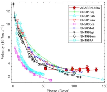
the blended trough could show an increasing blueward shift, as we see in ASASSN-15nx. On the other hand, the FeII lines, which are generally regarded as good tracers of the photosphere, show almost no variation during the entire spectral evolution. In Figure 19, the FeII line velocities of ASASSN-15nx are compared to other Type II SNe. Unlike the other SNe, the FeII velocity of ASASSN-15nx remains almost unchanged at ∼3.1 ´_{10 km s}3 -1_.

6. Summary of Peculiarities

ASASSN-15nx exhibits a number of unusual features, which can be summarized as follows.

Figure 17.Spectroscopic evolution in the velocity domain corresponding to the Hα and Hβ rest wavelengths. The FeIImultiplets are also in the Hβ window.

Figure 18.Velocity evolution of the Hβ, and FeIIlines for ASASSN-15nx. The velocities are estimated from the blueshift of the apparent absorption minima. No attempt has been made to decouple any possible contamination from other lines or high-velocity features.

Figure 19. Photospheric velocity evolution (vph) of ASASSN-15nx, as compared with other well-studied Type II SNe. The vphis estimated by the FeIIabsorption trough velocities.

marking the transition to a 56Co radioactive decay tail with a slope of 0.98 mag(100 day)−1.

3. The broadband colors are almost constant and remain blue after 50 days. Equivalently, the blackbody temper-ature monotonically decreases until day 50, as expected, reaching at T∼5.8 kK. However, after this epoch, we see an upward trend in the temperature, which reaches a value of ∼7.5 kK near day 135, before it again starts to decrease. Such an evolution has not been observed in any other SNeII.

4. The spectra of ASASSN-15nx shows unique, triangular Hα emission profile throughout its evolution. The strength of the Hα emission is weak, compared to a typical SN II-P/L.

5. The Hα profile shows no evidence for an associated P-Cygni absorption trough. The apparent absorption minima on the blue wing appears to be due to the presence of a SiII feature at day 53, and then an [OI] feature at later times.

6. Nebular spectral features like OI (7774 Å), [CaII] (ll 7291, 7324) and [OI] (ll 6300, 6364) appeared earlier than in a typical SN II-P/L. For example, the [OI] features in typical SNe IIP appear after ∼150 days, while they are detectable starting at day 87 in ASASSN-15nx. Due to the presence of these features, the spectra of ASASSN-15nx appear more evolved than a typical SN II at a similar age.

7. The OI(7774 Å) feature show a double-peaked emission at day 53. The unidentified redder component is much weaker at 87.4 days and completely disappears in later epochs. 8. The spectra all show an abrupt continuum break near

5500Å. The blue continuum is systematically brighter than the red (e.g., by ∼24% at 53.0 days).

9. There is a break in the blue wing of the both Hα and Hβ profiles (marked as “A1” and “A2” in Figures17and15),

starting at day 87, with a blueshifted velocity of ∼3.6 ´_{10 km s}3 -1_{, indicating that both of these features have a}

common HIorigin.

10. The Hβ velocity shows an unusual increasing trend with time. The Hβ absorption profile is also unusually broad and extended. This could not be reproduced by a single HIcomponent in our SYNOWmodels.

11. The FeIIline velocities show no evolution, while in typical SNe, all line velocities are expected to decay with time.

7. Discussion

We are not aware of a theoretical model that can explain all the peculiarities of ASASSN-15nx. Important questions remain, such as what powers this luminous SN II and how the long-lasting, “perfectly” linear light curve is produced, which are discussed in Sections7.1and7.2. In Section7.3, we comment on the rate of SNe that are like ASASSN-15nx.

be as high as 0.6–0.7M(e.g., for Type Ic SN 2011bm; Valenti

et al. 2012). The best-fit model also requires inefficient γ-ray

trapping, with t0γ≈71 days. For comparison, normal SNe IIP

are consistent with complete trapping (i.e.,t0g ¥), and for

SNe Ia, t0γ≈40 days (Wygoda et al.2017). The value of t0γfor

ASASSN-15nx implies that the envelope is inefficient at thermalizing the γ-rays. This is also consistent with weak Hα emission, because the hydrogen content in an SN ejecta is the dominant source of theγ-ray opacity.

The implied high56Ni mass and the short gamma-ray escape time of t0∼70days constrain the ejecta structure. The γ-rays

must escape the region in the ejecta where the 56Ni _is concentrated, allowing a constraint on the iron velocities. The gamma-ray escape time of a homogeneous ball of iron with outer velocity vedgeand mass M is

= ´ - ⎜ ⎟ ⎛ ⎝ ⎜ ⎞ ⎠ ⎟ ⎛_⎝ ⎞_⎠ ( ) t M M v 85 day 1.5 5 10 km s , 1 0 0.5 edge 3 1 1

using an effectiveγ-ray opacity of κ_γ= 0.025 cm2g−1(Swartz et al. 1995; Jeffery 1999). This implies that the produced iron

has to be distributed to velocities extending beyond ~ ´5

-10 km s3 1_{. Moreover, there is no room for significant additional}

mass at velocities  ´5 10 km s3 -1_{. Assuming that the hydrogen}

carries most of the energy, it is useful to write the constraint for additional mass at higher velocities in terms of the total energy. The gamma-ray escape time from the center of a homogeneous ball of hydrogen with kinetic energy E and mass M is

= - ⎛ ⎝ ⎜ ⎞ ⎠ ⎟⎛ ⎝ ⎜ ⎞ ⎠ ⎟ ( ) t M M E 87 day 2 10 erg . 2 0 ₅₁ 1 2

For example, a Ni mass of 1.5M extending to velocity

´

-7 10 km s3 1_{, embedded in a hydrogen ball of}  M 1 extending to16´10 km s3 -1_{, would have a total gamma-ray}

escape time of 70 days and total energy of 2×1051erg, which are not inconceivable.

To gain more insight into the envelope properties, we attempted a simple semi-analytical model described by Arnett (1980) and Arnett & Fu (1989). The formulation and

implementation of this model are discussed in Bose et al. (2015a) and references therein. This is a single-component

envelope model with radioactive 56Ni _{confined at the center.} This model is not fully applicable for ASASSN-15nx, as we observe no clear photospheric phase. However, by simply applying the model, we obtain an estimated envelope mass of ∼0.8–2.0 M with a thermal energy of ≈1.5×1051 erg. It

must be emphasized that these parameters are the upper limits; as these values increase, the model light curves show more sustained and prominent photospheric phases. For these para-meters, the ejecta becomes optically transparent at ∼45 days, which coincides with the break seen in the B-band light curve, after which the light curve is solely powered by the 56Ni



Co Fe

56 56 _{decay chain. This low ejecta mass is consistent with}

the inefficient γ-ray trapping required for the radioactive decay model. Although we see the presence of H, O and Ca lines in the late spectra, as we see in typical SNe II with large ejecta masses, these lines are much weaker than typical SNe II(see Figure16),

also suggestive of a low ejecta mass.

The large 56Ni_{mass is consistent with the correlation between} MNi and V-band luminosity, as shown in Figure 11. In this

scenario, ASASSN-15nx might have produced a tremendous amount of radioactive56Ni_{with a significantly stripped envelope.} However, it is not clear which mechanism could produce such a large mass of 56Ni_{. One possible scenario is a thermonuclear} explosion in a CCSNe (Kushnir 2015b; Kushnir & Katz2015),

which would produce a wide distribution of 56Ni_masses (Kushnir 2015a). Pair instability explosions can also produce a

large amount of 56Ni_{with a wide range of luminosities, but they} are also predicted to produce extended light curves (Kasen et al.2011) different from that observed for ASASSN-15nx.

The possible production of a large amount of56Ni_(∼0.6

 M ) in luminous and fast-declining SN II-L SN1979C was raised by Doggett & Branch(1985), Wheeler et al. (1987), and Young &

Branch(1989). Later, Blinnikov & Bartunov (1993) showed that

the high luminosity of SN1979C in its photospheric phase could also be explained by the reprocessing of UV light into optical by an extended low-mass hydrogen–helium envelope. However, despite the similarities in luminosity between ASASSN-15nx and SN1979C in its early phases, there is a clear break in the light-curve slope of SN1979C near 70 days that indicates a change in the dominant energy source. As the ejecta becomes optically thin, the UV reprocessing ceases. However, ASASSN-15nx does not show such a break, making it challenging to explain the prolonged, “perfectly” linear light curve of ASASSN-15nx solely by reprocessing of UV energy.

Another factor that may affect the 56Ni _{mass estimate is the} asymmetry of the ejecta. Höflich et al. (1999) showed that, for

Type Ic-BL supernova 1998bw, an ejecta axis ratio of 2 may produce 2 mag of variation in peak luminosity between the polar and equatorial directions. Polarimetric observations of SN1998bw were also consistent with asymmetry in the ejecta of 1998bw. Polarimetry studies suggest that CCSNe, particularly those with relatively small envelope masses, may exhibit significant asymmetry in their ejecta (see, e.g., Wang et al.

2001). If the ejecta of ASASSN-15nx were highly asymmetrical

and viewed at a favorable angle, the actual amount of synthesized Ni

56 _{might be substantially reduced from the current estimate and}

produce its high peak luminosity. On the other hand, there is no strong evidence of asymmetry in the [OI] (ll 6300, 6364) nebular lines, as suggested by Taubenberger et al.(2009,2013).

However, quantitative modeling is needed to investigate whether an asymmetric model could explain the prolonged linear light-curve and spectroscopic features of ASASSN-15nx.

Synthesizing a large amount of radioactive 56Ni _normally should also lead to nebular-phase spectra rich with iron-group elements, as seen in Type Ia SNe, but this doesn’t appear to be the case with ASASSN-15nx. This could pose a serious challenge to the high 56Ni _{mass scenario, and nebular-phase} spectral modeling would be needed to examine it further.

7.2. CSM Interaction

An alternative to the radioactive decay model is strong CSM interactions. In these models, the structure and distribution of the CSM can determine the shape of the light curves. As in SNeIIn

(Schlegel 1990), which are characterized by narrow emission

lines(FWHM∼few hundreds of km s-1_{) in the spectra, strong}

interactions are thought to be responsible for powering their prolonged and often luminous light curves (e.g., Smith et al.

2008a; Rest et al. 2011). Sometimes ejecta–CSM interactions

can lead to steeply declining light curves, as has been proposed for SN 2009jp (jet–CSM interaction; Smith et al. 2012a) and

ASASSN-15no (Benetti et al. 2018). PTF10iam (Arcavi

et al. 2016), which has early light curve features similar to

ASASSN-15nx, may also be explained by interaction.

The density profile of the CSM can be sculpted to produce the observed light curve of ASASSN-15nx. In ASASSN-15nx, we do not see narrow- or intermediate-width emission lines from the expanding shock driving photo-ionization of the remaining CSM. It is possible to miss such emission lines if those were only present before our spectroscopic observations began at 53.0 days. However, this seems unlikely, as the continuous and linear decline of the light curve indicates a single dominant powering source throughout the evolution, which should produce similar narrow emission lines at later phases if they were present earlier. On the other hand, sometimes CSM signatures may also remain hidden if there is asymmetry or the CSM has a velocity of several thousands of km s-1_.

Some of the spectral features in ASASSN-15nx can be attributed to indirect signatures of CSM interaction. TheSYNOW model could not reproduce the broad and extended Hβ absorption feature with a single, regular HI component, and the steadily increasing Hβ absorption velocity may indicate the presence of a blended high-velocity absorption component. In the case of CSM interactions relatively weaker than SNe IIn, the enhanced excitation of outer ejecta can produce high-velocity HIabsorption features(e.g., SNe 1999em, 2004dj (Chugai et al.2007), 2009bw

(Inserra et al.2012)) without producing narrow emission lines. In

some other cases, the interaction signature can remain blended with regular HIP-Cygni profiles: e.g., SNe 2012aw (Bose et al.

2013) and 2013ej (Bose et al.2015a), where the two components

can not be resolved individually, but result in broadening of Hα and Hβ absorption profiles. In ASASSN-15nx, as the strength of the regular component decays, the effective position of the blended absorption trough would shift blueward. However, this would also require a similar high-velocity absorption feature in the Hα profile, which does not seem to be present—instead, the entire absorption feature is missing in the SN. Another possibility is that this peculiar Hα emission line profile might be composed of multiple components arising from CSM interactions.

The unusual rise in temperature from 50 to 135 days, which also coincides with the period of steady increase in the Hβ velocity, might also be suggestive of CSM interaction. The increase in temperature could be due to the additional energy input from the ejecta interacting with CSM. The unusual break in the spectral continuum near 5500Å may be also explained via CSM interaction. Similar enhancements of the blue continuum have been seen in some strongly interacting SNe, such as SNe2011hw (Smith et al.2012b), 2006jc (Smith et al.2008b),

and 2005ip(Smith et al.2009). The blue excess could be due to

the blending of large number of broad and intermediate-width lines produced by the CSM interaction (Chugai 2009; Smith et al. 2012b). In the case of SN2005ip, the CSM lines were

narrow enough to be seen forming the blue excess.

Another possible signature indicative of CSM interaction is the A1 and A2 pair of features, discussed in Section 5.3 (see

We can make two simple estimates of the rate of transients that are similar to ASASSN-15nx: one based on a crude model of the ASAS-SN survey, and the other using a simple scaling based on the number of TypeIa SNe in ASAS-SN. Roughly speaking, ASAS-SN detects V<17 mag transients, which means that ASASSN-15nx could be detected to a comoving distance of ∼214Mpc, corresponding to a volume of V=0.041 Gpc3. The rate implied byfinding one such event is

p = W ⎜ ⎟ ⎛ ⎝ ⎞ ⎠ ⎛ ⎝ ⎜ ⎞ ⎠ ⎟ ( ) r t 25 4 years , 3 eff

whereW  2 is the fraction of the sky being surveyed for SNep at any given time and teffis the effective survey time. Roughly

speaking, ASAS-SN has been running for 2.7years, but finds only 70% of the V<17 mag SNe visible in its survey area, so



teff 1.8 years. Combining these factors gives a rough rate estimate of r; 28 Gpc−3yr−1. Alternatively, ASASSN-15nx is about one magnitude more luminous than a typical TypeIa SNe, implying an effective survey volume to find events like ASASSN-15nx that is four times greater than for TypeIa SNe. In itsfirst 2.7years, ASAS-SN found a total of 449 TypeIa SNe, so the rate for events like ASASSN-15nx should be r=rIa/4/449, correcting for the larger volume for detecting

ASASSN-15nx(4) and the ratio of the numbers of the two events (1 : 449). The TypeIa SNe rate isrIa3´104Gpc−3yr−1(Li et al.2011a), so r 17 Gpc−3yr−1, which is in good agreement with the first estimate. Thus, the rate of transients similar to ASASSN-15nx is comparable to that for hydrogen-poor(Type I) SLSNe rSLSN I- =91-+36

76

Gpc−3yr−1 derived by Prajs et al. (2017), raising the possibility that the previously identified

luminosity“gap” between normal CCSNe and SLSNe might be due to observational selection effects.

We thank A. Gal-Yam and M, Fraser for helpful comments. We are grateful to I. Arcavi for providing us the spectroscopic data for PTF10iam. S.B., S.D., and P.C. acknowledge Project 11573003, supported by the NSFC. S.B. is partially supported by the China Postdoctoral Science Foundation through grant No. 2016M600848. A.P., L.T., S.B., and N.E.R. are partially supported by the PRIN-INAF 2014 project“Transient Universe: Unveiling New Types of Stellar Explosions with PESSTO.” C.S.K., K.Z.S., and T.A.T. are supported by the U.S. National Science Foundation(NSF) though grants AST-1515927 and AST-1515876. We acknowledge support by the Ministry of Economy, Development, and Tourism’s Millennium Science Initiative through grant IC120009, awarded to The Millennium Institute of Astrophysics, MAS, Chile(J.L.P., C.R.-C.) and from CONICYT through FONDECYT grants 3150238 (C.R.-C.) and 1151445 (J.L.P.). Support for N.S. was provided by the NSF through grants 1312221 and AST-1515559 to the University of Arizona. A.M.G. acknowledges financial support by the University of Cádiz though grant PR2017-64.

Dame, the University of Minnesota, and the University of Virginia. We thank the staff at the MMT Observatory for their assistance with the observations. Observations using Steward Observatory facilities were obtained as part of the large observing program, AZTEC: Arizona Transient Exploration and Characterization. Some of the observations reported in this paper were obtained at the MMT Observatory, a joint facility of the University of Arizona and the Smithsonian Institution. Partially based on observations collected at Copernico telescope (Asiago, Italy) of the INAF— Osservatorio Astronomico di Padova.

This research was made possible through use of the AAVSO Photometric All-Sky Survey (APASS), funded by the Robert Martin Ayers Sciences Fund. This research uses data obtained through the Telescope Access Program (TAP), which has been funded by “The Strategic Priority Research Program: the Emergence of Cosmological Structures” of the Chinese Academy of Sciences(grant No. 11 XDB09000000) and the Special Fund for Astronomy from the Ministry of Finance.

We thank the Las Cumbres Observatory and its staff for their continuing support of the ASAS-SN project. We are grateful to M. Hardesty of the OSU ASC technology group. ASAS-SN is supported by the Gordon and Betty Moore Foundation through grant GBMF5490 to the Ohio State University and NSF grant AST-1515927. Development of ASAS-SN has been supported by NSF grant AST-0908816, the Mt. Cuba Astronomical Foundation, the Center for Cosmology and AstroParticle Physics at the Ohio State University, the Chinese Academy of Sciences South America Center for Astronomy(CASSACA), the Villum Foundation, and George Skestos. This paper uses data products produced by the OIR Telescope Data Center, supported by the Smithsonian Astrophysical Observatory.

The Liverpool Telescope is operated on the island of La Palma by Liverpool John Moores University in the Spanish Observatorio del Roque de los Muchachos of the Instituto de Astrofisica de Canarias, with financial support from the UK Science and Technology Facilities Council (STFC). This paper used data obtained with the MODS spectrographs built with funding from NSF grant AST-9987045 and the NSF Telescope System Instrumentation Program(TSIP), with additional funds from the Ohio Board of Regents and The Ohio State University Office of Research. The ModsIDL spectral data reduction reduction pipeline was developed in part with funds provided by NSF Grant AST-1108693. Partially based on observations collected at Copernico telescope (Asiago, Italy) of the INAF—Osservatorio Astronomico di Padova. The Joan Oró Telescope (TJO) of the Montsec Astronomical Observatory (OADM) is owned by the Catalan Government and operated by the Institute for Space Studies of Catalonia(IEEC).

Software: MATLAB, Python, IDL, SYNOW (Fisher et al.

1997,1999; Branch et al.2002), Astropy (Astropy Collaboration

et al.2013), IRAF (Tody1993), LT pipeline (Barnsley et al.2012; Piascik et al. 2014), DAOPHOT (Stetson 1987), FOSCGUI, modsIDL pipeline.

Table 1

Photometry of ASASSN-15nx

UT Date JD- Phasea B V R I g r i Telescopeb

2457,000 (days) (mag) (mag) (mag) (mag) (mag) (mag) (mag) /Inst.

2015 Jul 16.42 219.92 0.80 L >16.910 L L L L L ASASSN 2015 Jul 19.42 222.92 3.71 L 16.540±0.100 L L L L L ASASSN 2015 Jul 21.41 224.91 5.65 L 16.370±0.070 L L L L L ASASSN 2015 Jul 23.40 226.90 7.59 L 16.200±0.080 L L L L L ASASSN 2015 Aug 08.63 243.13 23.37 L 15.830±0.130 L L L L L ASASSN 2015 Aug 09.62 244.12 24.33 L 16.000±0.060 L L L L L ASASSN 2015 Aug 09.73 244.23 24.44 16.183±0.047 15.981±0.016 L 15.369±0.022 L L L LCO 2015 Aug 12.47 246.97 27.10 L 16.010±0.046 L 15.375±0.039 L L L LCO 2015 Aug 13.60 248.10 28.20 L 15.940±0.060 L L L L L ASASSN 2015 Aug 15.16 249.66 29.72 16.344±0.042 16.037±0.019 L 15.380±0.026 L L L LCO 2015 Aug 17.32 251.82 31.82 L 16.120±0.060 L L L L L ASASSN 2015 Aug 18.15 252.65 32.63 16.504±0.059 16.132±0.023 L 15.466±0.025 L L L LCO 2015 Aug 21.32 255.82 35.71 L L L 15.575±0.036 L L L LCO 2015 Aug 23.31 257.81 37.65 L 16.340±0.080 L L L L L ASASSN 2015 Aug 24.32 258.82 38.63 16.888±0.058 16.357±0.027 L 15.611±0.025 L L L LCO 2015 Aug 27.38 261.88 41.60 17.025±0.070 16.443±0.015 L 15.665±0.028 L L L LCO 2015 Aug 30.29 264.79 44.43 L L L 15.680±0.033 L L L LCO 2015 Sep 02.28 267.78 47.34 17.402±0.078 16.637±0.021 L 15.817±0.036 L L L LCO 2015 Sep 04.66 270.16 49.66 17.405±0.080 16.625±0.031 L 15.889±0.027 L L L LCO 2015 Sep 11.33 276.83 56.15 17.580±0.157 16.923±0.018 L L L L L LCO 2015 Sep 17.33 282.83 61.98 17.579±0.055 17.055±0.022 L 16.212±0.020 L L L LCO 2015 Sep 22.61 288.11 67.12 L L L 16.247±0.132 L L L LCO 2015 Sep 26.23 291.73 70.63 17.974±0.106 17.233±0.031 L 16.540±0.041 L L L LCO 2015 Sep 28.60 294.10 72.94 17.870±0.129 17.302±0.056 L 16.560±0.041 L L L LCO 2015 Oct 02.42 297.92 76.66 L 17.401±0.020 17.250±0.014 16.736±0.014 L L L LOTIS 2015 Oct 03.42 298.92 77.63 L 17.496±0.018 17.350±0.009 16.674±0.014 L L L LOTIS 2015 Oct 11.59 307.09 85.57 18.125±0.083 17.559±0.036 L 16.851±0.044 L L L LCO 2015 Oct 12.13 307.63 86.10 L L L L 17.829±0.005 17.551±0.008 17.464±0.008 NOT 2015 Oct 15.71 311.21 89.58 18.201±0.071 17.757±0.035 L 17.002±0.042 L L L LCO 2015 Oct 21.05 316.55 94.78 18.261±0.080 17.872±0.034 L 17.072±0.058 L L L LCO 2015 Oct 23.07 318.57 96.74 18.348±0.015 17.823±0.015 17.674±0.022 17.140±0.026 17.948±0.015 17.644±0.021 17.743±0.029 Coper,TJO 2015 Oct 25.88 321.38 99.47 L L L L L L L LCO 2015 Oct 29.40 324.90 102.89 L 18.017±0.070 L L L 17.927±0.070 17.961±0.076 LCO 2015 Nov 01.10 327.60 105.52 18.459±0.052 17.880±0.035 17.831±0.037 17.371±0.056 L L L TJO 2015 Nov 02.86 329.36 107.23 18.478±0.071 18.045±0.033 L L L 17.909±0.027 18.003±0.046 LCO 2015 Nov 05.17 331.67 109.48 18.635±0.024 18.216±0.016 L L 18.326±0.014 17.997±0.013 18.130±0.023 Coper 2015 Nov 07.08 333.58 111.34 18.690±0.023 18.092±0.032 17.980±0.029 17.496±0.038 L L L TJO 2015 Nov 07.32 333.82 111.57 L 18.303±0.036 18.085±0.021 17.741±0.047 L L L LOTIS 2015 Nov 07.35 333.85 111.60 18.684±0.077 18.262±0.035 L L L 18.038±0.026 18.110±0.048 LCO 2015 Nov 08.07 334.57 112.30 18.725±0.020 18.076±0.023 17.897±0.054 17.506±0.035 L L L TJO 2015 Nov 08.32 334.82 112.54 L 18.384±0.036 18.144±0.030 17.593±0.028 L L L LOTIS 2015 Nov 09.05 335.55 113.25 18.742±0.023 18.139±0.024 18.023±0.033 17.537±0.029 L L L TJO 2015 Nov 09.32 335.82 113.52 L 18.329±0.031 18.165±0.021 17.724±0.031 L L L LOTIS 2015 Nov 10.07 336.57 114.25 18.730±0.042 18.144±0.050 18.013±0.035 17.508±0.040 L L L TJO 2015 Nov 11.32 337.82 115.46 L 18.353±0.052 18.164±0.025 17.630±0.035 L L L LOTIS 2015 Nov 12.07 338.57 116.19 18.806±0.022 18.203±0.025 18.087±0.027 17.683±0.036 L L L TJO 2015 Nov 13.05 339.55 117.15 18.839±0.023 18.253±0.024 18.134±0.024 17.622±0.039 L L L TJO 15 Astrophysical Journal, 862:107 (19pp ), 2018 August 1 Bose et al.

2015 Nov 20.32 346.82 124.21 L 18.588±0.022 18.361±0.016 17.929±0.024 L L L LOTIS 2015 Nov 22.17 348.67 126.01 18.949±0.107 18.599±0.038 L L L 18.411±0.028 18.560±0.053 LCO 2015 Nov 23.32 349.82 127.13 L L L 17.936±0.573 L L L LOTIS 2015 Nov 27.32 353.82 131.02 L 18.687±0.097 18.815±0.060 18.033±0.047 L L L LOTIS 2015 Nov 28.02 354.52 131.70 L L L L L L L LCO 2015 Nov 29.32 355.82 132.97 L 18.825±0.047 18.681±0.040 18.049±0.044 L L L LOTIS 2015 Nov 29.52 356.02 133.16 19.230±0.093 18.739±0.037 L L L 18.538±0.039 18.883±0.086 LCO 2015 Nov 30.51 357.01 134.13 19.128±0.074 18.771±0.034 L L L 18.570±0.035 18.843±0.057 LCO 2015 Dec 03.02 359.52 136.56 19.207±0.042 18.833±0.026 L L 19.082±0.034 18.620±0.016 18.882±0.024 Coper 2015 Dec 03.33 359.83 136.87 L 18.951±0.045 18.695±0.031 18.270±0.041 L L L LOTIS 2015 Dec 03.63 360.13 137.16 L 18.713±0.063 L L L L L LCO 2015 Dec 06.84 363.34 140.28 19.211±0.100 18.886±0.041 L L L 18.707±0.037 18.852±0.081 LCO 2015 Dec 07.33 363.83 140.76 L 18.778±0.105 18.790±0.103 L L L L LOTIS 2015 Dec 09.64 366.14 143.00 L 18.759±0.104 L L L L L LCO 2015 Dec 10.33 366.83 143.67 L 19.002±0.051 18.877±0.047 18.277±0.066 L L L LOTIS 2015 Dec 13.98 370.48 147.23 19.579±0.122 19.106±0.066 L L L 18.899±0.056 L LCO 2015 Dec 16.33 372.83 149.51 L 19.255±0.063 19.029±0.033 18.587±0.099 L L L LOTIS 2015 Dec 18.01 374.51 151.14 19.621±0.042 19.346±0.043 L L 19.362±0.020 19.008±0.035 L Coper 2015 Dec 18.28 374.78 151.40 L 19.243±0.048 L L L 19.075±0.046 L LCO 2015 Dec 18.90 375.40 152.01 L 19.217±0.024 L L 19.388±0.021 19.033±0.020 19.378±0.027 Coper 2015 Dec 19.33 375.83 152.43 L 19.349±0.068 19.188±0.076 L L L L LOTIS 2015 Dec 23.86 380.36 156.83 L 19.225±0.180 L L L 19.253±0.214 L LCO 2015 Dec 27.88 384.38 160.74 19.815±0.041 19.445±0.036 L L L 19.198±0.028 19.495±0.039 LT 2015 Dec 28.21 384.71 161.06 20.114±0.186 19.464±0.049 L L L 19.189±0.041 19.446±0.084 LCO 2015 Dec 30.24 386.74 163.04 L 19.528±0.213 L L L 19.177±0.099 19.368±0.107 LCO 2016 Jan 01.27 388.77 165.01 L 19.630±0.048 19.440±0.047 19.046±0.080 L L L LOTIS 2016 Jan 03.27 390.77 166.96 L 19.833±0.146 19.475±0.097 18.889±0.088 L L L LOTIS 2016 Jan 05.92 393.42 169.53 20.198±0.021 19.573±0.018 L L L 19.391±0.016 19.601±0.022 LT 2016 Jan 10.94 398.44 174.41 20.347±0.017 19.719±0.017 L L L 19.574±0.013 19.761±0.025 LT 2016 Jan 12.27 399.77 175.71 L 19.876±0.145 L L L L L LOTIS 2016 Jan 16.90 404.40 180.21 20.487±0.051 19.842±0.042 L L L 19.697±0.028 L LT 2016 Jan 18.20 405.70 181.48 L 19.743±0.147 19.633±0.089 L L L L LOTIS 2016 Jan 21.87 409.37 185.05 20.546±0.107 L L L L L L LT 2016 Jan 26.89 414.39 189.93 20.783±0.016 20.192±0.018 L L L 20.038±0.014 20.242±0.027 LT 2016 Jan 27.13 414.63 190.16 L 20.187±0.155 19.931±0.076 19.464±0.115 L L L LOTIS 2016 Jan 30.13 417.63 193.08 L 20.244±0.095 20.226±0.085 19.748±0.120 L L L LOTIS 2016 Feb 05.13 423.63 198.91 L 20.320±0.186 L L L L L LOTIS 2016 Feb 08.13 426.63 201.83 L 20.478±0.149 L 19.784±0.213 L L L LOTIS 2016 Feb 11.10 429.60 204.72 L 20.468±0.117 20.523±0.102 L L L L LOTIS 2016 Feb 24.13 442.63 217.39 L 20.729±0.049 L L L L L MDM 2016 Feb 25.12 443.62 218.36 L 20.625±0.030 L L L L L MDM 2016 Mar 03.85 451.35 225.87 L L L L L 20.768±0.082 L LT 16 (19pp ), 2018 August 1 Bose et al.

Table 1 (Continued)

UT Date JD- Phasea _{B V R I g r i Telescope}b

2457,000 (days) (mag) (mag) (mag) (mag) (mag) (mag) (mag) /Inst.

2016 Mar 04.85 452.35 226.85 L L L L L 20.819±0.094 L LT

2016 Mar 09.87 457.37 231.73 L 20.924±0.045 L L L L L LT

2016 Mar 12.10 459.60 233.90 L 21.182±0.022 L L L L L Mag

2016 Mar 15.88 463.38 237.58 L 21.213±0.029 L L 21.598±0.049 21.163±0.033 20.977±0.033 LT, NOT

2016 Apr 09.99 488.49 261.99 22.290±0.060 21.709±0.049 L L L 21.491±0.028 21.317±0.043 Mag

Notes.Data observed within 5 hr are represented under a single-epoch observation. a

Rest-frame days with reference to the explosion epoch JD2457219.10. b

The abbreviations of telescope/instrument used are as follows: ASASSN—ASAS-SN quadruple 14 cm telescopes; LCO—Las Cumbres Observatory 1 m telescope network; LT—2 m Liverpool Telescope; NOT— ALFOSC mounted on 2.0 m NOT telescope; MDM—2.4 m MDM telescope; LOTIS—0.6 m Super-Lotis telescope; TJO—0.8 m TJO telescope; Coper—1.8 m Copernico telescope; Mag—IMACS mounted on 6.5 m Magellan Baade telescope.

17 Astrophysical Journal, 862:107 (19pp ), 2018 August 1 Bose et al.