DOTTORATO DI RICERCA IN
INGEGNERIA CIVILE, AMBIENTALE E DEI MATERIALI
Ciclo XXVIII
Settore Concorsuale di afferenza: 08/A3 Settore Scientifico disciplinare: ICAR/04
DEVELOPMENT OF NEW METHODOLOGIES FOR PREDICTION
OF PERFORMANCES OF ASPHALT MIXTURES
Candidato: Dott. Ing. RICCARDO LAMPERTI
Coordinatore Dottorato
Relatori
Prof. Ing. Alberto Lamberti
Prof. Ing. Andrea Simone
Dott. Ing. Valeria Vignali
I This thesis proposes the use of new methodologies for prediction of performances of asphalt mixtures.
Recent improvements in technology make it possible to adopt new methods of investigation with the dual objective of improving the performance in the survey of the parameters and investigate new properties so far not analyzed. In particular, the image analysis and the tyre/surface interaction belong to an innovative framework, which is next to flank, if not replace, the classic measurements so far employed.
The thesis deals with the use of these technologies for the analysis of three rubberized stone mastic asphalts, which were laid on a stretch of road close to Bologna, Italy. Three different surveys were carried out on site during the first year of service. The surveys included the change in texture and skid resistance due to the traffic, along with the acoustic properties of the pavement. Local as well as dynamic continuous measurements were carried out, involving the use of a profilometer and a skiddometer. A second phase involved the prediction of the surface parameters with simulated trafficking on Road Test Machine. At each stage of simulated trafficking, change in macrotexture, skid resistance, adhesion between bitumen and aggregates and finally contact pressures and areas were assessed.
The image analysis is used for the assessment of the adhesion between the bitumen and the aggregate. The proposed procedure overcomes the shortcomings of the current evaluation, offering great reliability and accuracy.
The images are then processed in order to create 3D models of the asphalt specimens and investigate the surface and volume properties.
The tyre/pavement interaction is another fundamental phenomena that received little considerations from the research, given its importance.
A final discussion summarizes these investigations by separately review three different simulated periods, i.e. the early life, the in-service equilibrium and the end of life. In order to accelerate the distress, one slab was subjected to Immersion Wheel Track test, the results of which were interpreted through the same methodologies.
III Questa tesi propone l’utilizzo di nuove metodologie per predire le prestazioni di conglomerati bituminosi.
I recenti progressi nella tecnologia rendono possibile adottare nuovi metodi di indagine con il duplice obiettivo di migliorare il rendimento del rilievo dei parametri e approfondire nuove caratteristiche ancora non studiate. In particolare, l’analisi delle immagini e l’interazione ruota/pavimentazione appartengono ad un contesto innovativo destinato ad affiancare, se non a sostituire, i metodi classici di indagine finora impiegati.
La tesi tratta l’impiego di queste tecnologie per l’analisi di tre miscele di stone mastic asphalt contenenti polverino di gomma, le quali sono state stese in un tratto stradale vicino a Bologna.
Nell’arco temporale di un anno dopo la stesa sono stati effettuati tre differenti rilievi. Essi hanno permesso di indagare l’evoluzione dei parametri di tessitura, attrito e riduzione del rumore di rotolamento. Sono state effettuate misure puntuali e dinamiche in continuo mediante l’utilizzo di un profilometro e dello skiddometer.
Una seconda fase ha previsto la stima dei parametri superficiali a seguito di trafficamento simulato in laboratorio. Ad ogni livello sono stati determinati i cambiamenti di macrotessitura, attrito, adesione bitume inerte, nonché le pressioni e l’area di contatto. L’analisi delle immagini è usata per determinare l’adesione tra inerte e bitume. La procedura proposta supera le limitazioni della valutazione visiva, offrendo grande affidabilità e precisione.
Le immagini sono seguentemente combinate per creare modelli 3D dei campioni di conglomerato e studiare i parametri superficiali e volumetrici.
L’interazione ruota pavimentazione è un altro fenomeno fondamentale che, nonostante la sua importanza, ha ricevuto poca considerazione dalla ricerca.
La discussione finale sintetizza i vari aspetti esaminati raggruppando tre diverse “età” della pavimentazione, ovvero inizio vita, equilibrio e fine vita o ammaloramento. Al fine di accelerare il processo di ammaloramento, un campione è stato sottoposto a wheel track ad immersione, interpretando i risultati con le stesse metodologie.
V Abstract ... I Abstract ... III List of Figures ... X List of Tables...XX Introduction ... 1
Chapter 1 - Texture and skid resistance ... 3
1.1 Texture of road pavement... 3
1.1.1 Microtexture ... 4
1.1.2 Macrotexture ... 5
1.1.3 Megatexture ... 6
1.2 Measurement of pavement surface texture ... 6
1.2.1 Contact ... 6
1.2.2 Non-contact ... 7
1.3 Surface metrology on road pavements ... 9
1.4 Skid resistance ... 12
1.5 Measurement of skid resistance ... 13
1.6 PIARC harmonization – IFI index ... 16
Chapter 2 - Literature review ... 19
2.1 Texture... 19
2.1.1 A comparison of techniques to determine surface texture data ... 20
2.1.2 A study on texture and acoustic properties of cold laid microsurfacings………...21
2.1.3 Changes of surface dressing texture as related to time and chipping size…….. ... 23
2.2 Skid resistance ... 25
2.2.1 An assessment of the skid resistance effect on traffic safety under wet -pavement conditions ... 26
2.2.2 Mobile laser scanning system for assessment of the rainwater runoff and drainage conditions on road pavements ... 28
2.2.3 Geometric texture indicators for safety on AC pavements with 1 mm 3D laser texture data ... 32
VI 2.3.2 The wear of Stone Mastic Asphalt due to slow speed high stress
simulated laboratory trafficking ... 37
2.3.3 Durable laboratory rubber friction test countersurfaces that replicate the roughness of asphalt pavements ... 38
2.4 Recycling and sustainability of road pavements ... 41
2.4.1 Stone Mastic Asphalts ... 41
2.4.1.1 Evaluation of SBS modified stone mastic asphalt pavement performance ... 41
2.4.1.2 Comparison of performance of stone matrix asphalt mixtures using basalt and limestone aggregates ... 42
2.4.2 The art of recycling into road mixtures ... 44
2.4.3 Use of crumb-rubber into road mixtures ... 46
2.4.3.1 Evaluating the effects of the wet and dry processes for including crumb rubber modifier in hot mix asphalt ... 46
2.4.3.2 Improvement of Pavement Sustainability by the Use of Crumb Rubber Modified Asphalt Concrete for Wearing Courses ... 49
2.4.3.3 The mechanical performance of dry-process crumb rubber modified hot bituminous mixes: The influence of digestion time and crumb rubber percentage ... 50
2.5 Acoustic properties of pavements ... 53
2.5.1 A modified Close Proximity method to evaluate the time trends of road pavements acoustical performances ... 53
2.5.2 Noise Abatement of Rubberized Hot Mix Asphalt: A Brief Review ... 54
2.5.3 The effects of pavement surface characteristics on tire/pavement noise 56 2.5.4 Road pavement rehabilitation using a binder with a high content of crumb rubber: Influence on noise reduction ... 58
2.5.5 Durability and variability of the acoustical performance of rubberized road surfaces ... 60
Chapter 3 - Materials characterization ... 63
3.1 Mixtures characterization ... 63
3.2 Quality acceptance controls: mechanical characterization ... 67
Chapter 4 - The trial site ... 71
VII
4.2.2 Site survey and results ... 77
Chapter 5 - Site surveys ... 83
5.1 Noise measurements ... 83
5.1.1 Test method ... 83
5.1.2 Results ... 84
5.2 Texture and skid resistance ... 91
5.2.1 Static measurements ... 91
5.2.1.1 Skid resistance ... 93
5.2.1.2 Macrotexture ... 100
5.2.2 Dynamic advanced measurements ... 104
5.2.2.1 Skiddometer ... 104
5.2.2.1.1 Equipment and test methods ... 104
5.2.2.1.2 Results ... 106
5.2.2.2 LaserProf ... 108
5.2.2.2.1 Equipment and test methods ... 108
5.2.2.2.2 Results ... 111
Chapter 6 - Laboratory simulated trafficking and classic measurements ... 115
6.1 Introduction ... 115
6.2 Road Test Machine ... 116
6.3 Immersion wheel track ... 117
6.4 Mean Texture Depth – EN 13036-1 ... 119
6.5 Pendulum Test – EN 13036-4 ... 121
Chapter 7 - 2D Image analysis ... 125
7.1 Introduction ... 125
7.2 ImageJ overview... 126
7.3 Analysis procedure ... 126
7.4 Rolling Bottle test on different coloured aggregates ... 131
7.5 Effect of rubber on adhesion ... 136
7.5.1 Rolling Bottle test ... 136
7.5.2 Simulated trafficking – RTM and IWT... 137
VIII
8.2.1 Introduction ... 142
8.2.2 3D model creation ... 143
8.3 Surface imaging analysis – MountainsMap ... 150
8.4 Preliminary analysis ... 151
8.5 Results - Texture change with trafficking ... 156
8.5.1 Abbott-Firestone Curve and surface heights parameters ... 156
8.5.1.1 Comparison between the slabs ... 157
8.5.1.2 RTM versus IWT ... 161
8.5.2 Void volume and projected Area ... 164
8.5.2.1 Comparison between the slabs ... 164
8.5.2.2 RTM versus IWT ... 167
8.5.3 Slice study ... 172
8.5.4.1 Comparison of the three different slabs ... 172
8.5.4.2 RTM versus IWT ... 178
8.5.5 Use of vinyl material to replicate asphalt surface macrotexture ... 183
Chapter 9 - The tyre – pavement interaction ... 187
9.1 Introduction ... 187
9.2 Test description ... 187
9.3 Understanding tyre/surface interaction ... 188
9.4 Ideal surfaces ... 196
9.5 Different asphalt surfaces ... 201
9.6 Rubberized 8 mm SMA ... 204 9.6.1 8 mm SMA 0.00 ... 205 9.6.2 8 mm SMA 0.75 ... 207 9.6.3 8 mm SMA 1.20 ... 212 Chapter 10 - Discussion ... 215 10.1 Introduction ... 215 10.2 Texture evolution ... 215
10.2.1 Early life evolution ... 217
10.2.2 Mid-life ... 220
X Figure 1.1: Texture wavelengths and relationship with pavement surface characteristics Figure 1.2: Positive and negative texture
Figure 1.3: Mean Profile Depth calculation
Figure 1.4: Reconstructed 3D surface of an asphalt sample Figure 1.5: Concept of Material Ratio
Figure 1.6: Abbott curve for a single profile and parameters Rk, Rpk and Rvk Figure 1.7: Abbott curve for a surface and parameters Sk, Spk, Svk
Figure 3.1: Grading curves of the mixtures
Figure 3.2: Sampling of material during the laying
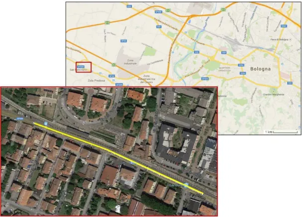
Figure 4.1: Aerial view and location of the trial site in Zola Predosa Figure 4.2: Plant of the experimental site
Figure 4.3: Laying and compaction phases of the SMA
Figure 4.4: Temperature verification during laying: no rubber on the left, with rubber on the right
Figure 4.5: Environmental and cutaneous surveys Figure 4.6: Environmental survey – PAHs
Figure 4.7: PAHs concentration survey for workers Figure 4.8: Breathable dust survey for workers
Figure 4.9: PAHs measured with dermal patch applied on workers Figure 5.1: Lcpx dir. Bologna measured at 50 Km/h for SMA 0 Figure 5.2: Lcpx dir. Modena measured at 50 Km/h for SMA 0.75 Figure 5.3: Lcpx dir. Modena measured at 50 Km/h for SMA 1.20 Figure 5.4: Emission spectra for SMA 0.00
XI Figure 5.6: Emission spectra for SMA 1.20
Figure 5.7: Evolution of the average Lcpx measured at 40 km/h Figure 5.8: Evolution of the average Lcpx measured at 50 km/h Figure 5.9: Evolution of the average Lcpx measured at 80 km/h Figure 5.10: Difference between Lcpx of 0.75 SMA and SMA 0.00 Figure 5.11: Difference between Lcpx of 1.20 SMA and SMA 0.00
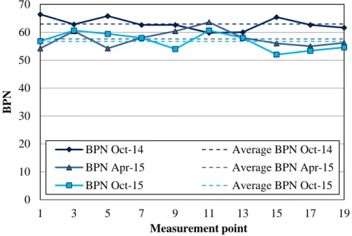
Figure 5.12: BPN measured at different locations during the surveys for SMA 0 Figure 5.13: Position of the measuring section for the static measurements Figure 5.14: BPN measured at different locations during the surveys for SMA 0 Figure 5.15: BPN measured at different locations during the surveys for SMA 0.75 Figure 5.16: BPN measured at different locations during the surveys for SMA 1.20 Figure 5.17: Summary of the average BPN measured during the surveys for the three mixtures
Figure 5.18: PTV measured at different locations during the surveys for SMA 0 Figure 5.19: PTV measured at different locations during the surveys for SMA 0.75 Figure 5.20: PTV measured at different locations during the surveys for SMA 1.20 Figure 5.21: Summary of the average PTV measured during the surveys for the three mixtures
Figure 5.22: MTD measured at different locations during the surveys for SMA 0 Figure 5.23: MTD measured at different locations during the surveys for SMA 0.75 Figure 5.24: MTD measured at different locations during the surveys for SMA 1.20 Figure 5.25: Summary of the average MTD measured during the surveys for the three mixtures
XII Figure 5.28: BFC for the rubberized SMA surfaces
Figure 5.29: Laseprof equipment for MPD survey
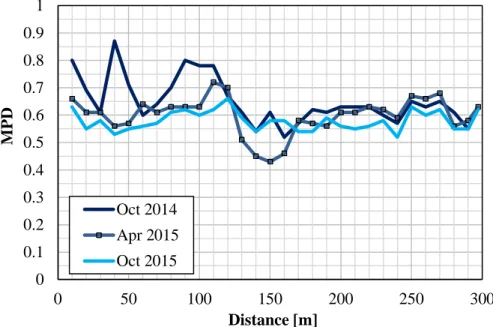
Figure 5.30: MPD for the reference Stone Mastic Asphalt with no rubber Figure 5.31: MPD for the rubberized SMA surfaces
Figure 5.32: ETD for the reference Stone Mastic Asphalt with no rubber Figure 5.33: ETD for the rubberized SMA surfaces
Figure 6.1: Road Test Machine Figure 6.2: Immersion Wheel Track
Figure 6.3: Treaded tyre used for the Immersion Wheel Track
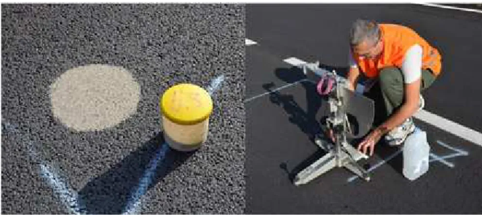
Figure 6.4: Sand placed onto the surface (left) and evenly spread for measuring MTD Figure 6.5: MTD versus wheel passes for early 8 mm SMA life
Figure 6.6: MTD versus wheel passes for 8 mm SMA life Figure 6.7: Steel frame for detecting the area of testing
Figure 6.8: Pendulum test. a) the surface is free; b) the slider is in contact with the surface; c) the arm is hold before it swings back to the surface
Figure 6.9: Number of Swings before reaching PTV
Figure 6.10: PTV versus wheel passes for the different 8 mm SMA Figure 7.1: Set for digital picturing of tested samples
Figure 7.2: Image filtering process. a) original image; b) non-classified image; c) classified image
Figure 7.3: Validation of the technique: pixels’ color inspection for the non-classified (a) and classified (b) images
XIII Figure. 7.6: Results of rolling bottle tests after 6 hours (a) and 24 hours testing (b)
Figure 7.7: Loss of rubber during the Rolling Bottle test
Figure 7.8: Results of the rolling bottle test on bitumen – rubber – aggregate blends Figure 7.9: Picture improvement through Lightroom®
Figure 7.10: Picture analysis with ImageJ
Figure 7.11: Areas selection process with ImageJ
Figure 7.12: Development of the adhesion with trafficking for SMA surfaces Figure 8.1: CRP acquisition method for slabs
Figure 8.2: Initial Zephyr screen
Figure 8.3: Zephyr window 1 and 3 (control points and distances) Figure 8.4: Picture loading window
Figure 8.5: Camera orientations Figure 8.6: Sparse point cloud Figure 8.7: Dense point cloud Figure 8.8: Final mesh
Figure 8.9: Final mesh Figure 8.10: Final mesh Figure 8.11: Final mesh
Figure 8.12: different gradations of SMA under study Figure 8.13: Void volume and material volume parameters Figure 8.14: Vmp versus lower bearing ratio
XIV Figure 8.17: Vmp5 versus PTV
Figure 8.18: Vmp80 versus MTD Figure 8.19: Vmp80 versus Sa
Figure 8.20: 3D Models of the 0.75 slab at different trafficking stages - RTM
Figure 8.21: 3D Models of the 0.75 slab at different trafficking stages – end of RTM and IWT
Figure 8.22: Volume of material peak 5% low limits for 8 mm slabs, early life Figure 8.23: Volume of material peak 5% low limits for 8 mm slabs
Figure 8.24: Volume of material core 5% low limit for 8 mm SMA Figure 8.25: Volume of void 5% low limit for 8 mm slabs
Figure 8.26: Sk for 8 mm slabs
Figure 8.27: Sa for 8 mm slabs, early life Figure 8.28: Sa for 8 mm slabs
Figure 8.29: Volume of material peak 5% low limits for 0.75 slab Figure 8.30: Volume of material core 5% low limit for 0.75 slab Figure 8.31: Volume of void 5% low limit for 0.75 slab
Figure 8.32: Sk for 0.75 slab Figure 8.33: Sa for 0.75 slab
Figure 8.34: Sa versus Vmp80 for 0.75 slab Figure 8.35: Volume of void low for 0.00 slab
Figure 8.36: Projected Area along height for 0.00 slab Figure 8.37: Volume of void low for 1.20 slab
XV Figure 8.40: Volume of void low for 0.75 slab
Figure 8.41: Volume of void distribution along height for 0.75 slab, early life Figure 8.42: Volume of void along height for 0.75 slab
Figure 8.43: Volume of void along height for 0.75 slab during IWT
Figure 8.44: Volume of void along height summary for 0.75 slab during RTM and IWT Figure 8.45: Projected Area along height summary for 0.75 slab during RTM
Figure 8.46: Projected Area along height summary for 0.75 slab during IWT Figure 8.47: Projected Area trend versus time at different depth for IWT test
Figure 8.48: Projected Area along height summary for 0.75 slab during RTM and IWT Figure 8.49: Volume of material high for 8 mm slabs, early life
Figure 8.50: Volume of material high for 8 mm slabs Figure 8.51: Volume of void high for 8 mm slabs, early life Figure 8.52: Volume of void high for 8 mm slabs
Figure 8.53: Volume of material median for 8 mm slabs, early life Figure 8.54: Volume of material median for 8 mm slabs
Figure 8.55: Volume of void median for 8 mm slabs, early life Figure 8.56: Volume of void median for 8 mm slabs
Figure 8.57: Volume of material low for 8 mm slabs, early life Figure 8.58: Volume of material low for 8 mm slabs
Figure 8.59: Volume of void low for 8 mm slabs, early life Figure 8.60: Volume of void low for 8 mm slabs
Figure 8.61: Slice study: map evolution for 0.75 slab, RTM Figure 8.62: Slice study: map evolution for 0.75 slab, IWT
XVI Figure 8.64: Volume of void high for 0.75 slab
Figure 8.65: Volume of material median for 0.75 slab Figure 8.66: Volume of void median for 0.75 slab Figure 8.67: Volume of material low for 0.75 slab Figure 8.68: Volume of void low for 0.75 slab
Figure 8.69: Pouring the hot vinamold onto the slab surface Figure 8.70: Peeling off the hot vinamold from the slab surface
Figure 8.71: Comparison of Volume of void for original and vinyl replicate samples Figure 8.72: Comparison of Projected Area for original and vinyl replicate samples Figure 9.1: Equipment for the tyre/surface interaction analysis
Figure 9.2: Positions of the GripTester tyre for the preliminary assessment Figure 9.3: Contact patch of a reference smooth glass
Figure 9.4: Load applied to the end of the level arm versus width of the tyre footprint Figure 9.5: Load applied to the end of the level arm versus height of the tyre footprint Figure 9.6: Load applied to the end of the level arm versus contact patch area of the tyre Figure 9.7: Load applied to the end of the level arm versus average pressure
Figure 9.8: Inflation pressure versus average measured pressure Figure 9.9: Average measured pressure versus contact patch area Figure 9.10: Inflation pressure versus contact patch area
Figure 9.11: Average measured pressure versus load applied Figure 9.12: Contact area versus load applied
Figure 9.13: Contact patch of a rejected tyre Figure 9.14: Small and big tiles mosaics
XVII Figure 9.16: Pressure distribution strip for the glass
Figure 9.17: Pressure distribution strip for the big tiles. Wheel centred on the tiles (T.C.) Figure 9.18: Pressure distribution strip for the big tiles. Wheel centred on the groove (G.C.)
Figure 9.19: Pressure distribution strip for the small tiles. Wheel centred on the tiles (T.C.) Figure 9.20: Pressure distribution strip for the small tiles. Wheel centred on the groove (G.C.)
Figure 9.21: Pressure distribution strip for the small tiles. Wheel centred on the groove (G.C.)
Figure 9.22: Frequency distribution comparison for glass and tiles Figure 9.23: Cumulative frequency comparison for glass and tiles Figure 9.24: Cumulative frequency comparison for different surfaces Figure 9.25: Comparison of pressure and contact area for different surfaces Figure 9.26: Pressure frequency distribution for different surfaces
Figure 9.27: High-pressure frequency distribution for different surfaces Figure 9.28: Cumulative frequency distribution for different surfaces
Figure 9.29: Frequency distribution comparison for different trafficked 8 mm 0.00 SMA specimen
Figure 9.30: Cumulative frequency comparison for different trafficked 8 mm 0.00 SMA specimens
Figure 9.31: Magnification of the density distribution tail for 8 mm 0.00 SMA specimen Figure 9.32: Magnification of the high-pressure area for 8 mm 0.00 SMA specimens Figure 9.33: Early life pressure maps evolution for 0.75 SMA
XVIII Figure 9.36: Magnification of the most frequent pressure area for 8 mm 0.75 SMA specimens
Figure 9.37: Cumulative frequency comparison for different trafficked 8 mm 0.75 SMA specimens
Figure 9.38: Magnification of the high-pressure area for 8 mm 0.75 SMA specimens Figure 9.39: Frequency distribution comparison for different trafficked 8 mm 1.20 SMA specimens
Figure 9.40: Magnification of the most frequent pressure area for 8 mm 1.20 SMA specimens
Figure 9.41: Cumulative frequency comparison for different trafficked 8 mm 1.20 SMA specimens
Figure 9.42: Magnification of the high-pressure area for 8 mm 1.20 SMA specimens Figure 10.1: Skewness of a surface
Figure 10.2: Example of a periodic texture, with Ssk value 0.16, Sku value 1.63 Figure 10.3: Example of a spiky texture, with Ssk value 3.20, Sku value 18.71 Figure 10.4: Skewness versus wheel passes, early life
Figure 10.5: Kurtosis versus wheel passes, early life
Figure 10.6: Pictures of the 0.75 SMA surface after 100 and 5000 wheel passes Figure 10.7: Contact area versus wheel passes
Figure 10.8: Early life 3D models of SMA 1.20 slab Figure 10.9: Skewness versus wheel passes
Figure 10.10: Kurtosis versus wheel passes Figure 10.11: Contact area versus wheel passes
XIX Figure 10.14: Skewness and kurtosis for the SMA 0.75
Figure 10.15: 3D model of the SMA 0.75 after 225 minutes of IWT
Figure 10.16: Frequency distribution of the tyre pavement interaction pressure for the SMA 0.75
Figure 10.17: Cumulative frequency of the tyre pavement interaction pressure for the SMA 0.75
Figure 10.18: Pressure map of the SMA 0.75 slab at the end of RTM and IWT test (pressure legend: 68.95 ÷ 399.9 kPa)
Figure 10.19: Pressure map of the SMA 0.75 slab at the end of IWT test (pressure legend: 68.95 ÷ 703.26 kPa)
XX Table 1.1: Texture wavelengths
Table 1.2: Slider friction measurement devices
Table 1.3: Locked Wheel friction measurement devices Table 1.4: Side Force friction measurement devices Table 1.5: Fixed slip friction measurement devices
Table 1.6: Variable - Fixed slip friction measurement devices Table 3.1: Physical characteristics of asphalt mixtures
Table 3.2: Volumetric properties after Marshall compaction Table 3.3: Water damage and Cantabro tests
Table 3.4: Marshall properties after 50 blows
Table 3.5: Indirect tensile results on Marshall specimens at 60°C
Table 3.6: ITSM results on Marshall specimens at different temperatures Table 3.7: ITSM results on Marshall specimens at different temperatures Table 3.8: Physical characteristics of asphalt mixtures
Table 3.9: Volumetric properties after Marshall compaction Table 3.10: Marshall test after 50 blows of compaction
Table 3.11: Indirect tensile results on Marshall specimens at 60°C Table 3.12: Volumetric properties after different compaction gyrations Table 3.13: Indirect tensile test on gyratory compacted samples at 25°C Table 3.14: Average ITSM
XXI Table 5.1: PTV statistics for SMA 0
Table 5.2: PTV statistics for SMA 0.75 Table 5.3: PTV statistics for SMA 1.20 Table 5.4: MTD statistics for SMA 0 Table 5.5: MTD statistics for SMA 0.75 Table 5.6: MTD statistics for SMA 1.20
Table 5.7: coefficients adopted for IFI calculation Table 5.8: Summary of BFC during the surveys Table 5.9: Laseprof equipment for MPD survey
Table 5.10: ETD classification according to CNR 94/1983 Table 5.11: Summary of MPD over the surveys
Table 5.12: Summary of ETD over the surveys
Table 7.1 Accuracy indexes for a matrix with k classes Table 7.2: YUV ranges for materials’ recognition
Table 7.3: Confusion matrix and accuracy indexes for Limestone Table 7.4: Confusion matrix and accuracy indexes for Porphyry Table 7.5: Confusion matrix and accuracy indexes for Basalt
Table 7.6: Confusion matrix and accuracy indexes for Blast furnace slag Table 7.7: OA and BAA indexes for the tested aggregates
1 The pavement engineering industry is facing a continuous change nowadays. The concept of sustainability is becoming of paramount importance in any field of research and has become one of the main goal of the researchers, favoured by the recent legislative measures and the public opinions. By way of example, the last International Conference on Transportation Infrastructures, held in Pisa in 2014, dealt with the “Sustainability, Eco-Efficiency, and Conservation in Transportation Infrastructure Asset Management”. Efforts are made throughout the world in identifying suitable recycled materials for the use in road pavements. Among them, one of the most reused material is the crumb rubber, which was the subject of numerous studies.
Moreover, recent improvements in technology make it possible to adopt new methods of investigation with the dual objective of improving the performance in the survey of the parameters and investigate new properties so far not analysed.
For instance, the use of non-contact methods based on the image analysis and processing for 3D reconstruction, has potential for highway monitoring and maintenance.
The tyre/pavement interaction is another fundamental phenomena that received little considerations from the research, given its importance.
These techniques can be very useful for a better understanding of pavement surface texture properties such as skid resistance, road surface noise and rolling resistance.
This thesis proposes the use of new technologies for the analysis of surface characteristics of road pavements. In particular, the study was carried out on three mixtures of rubberized Stone Mastic Asphalts, which have been laid on a stretch of road close to Bologna (Italy). It is shown that the technologies adopted and the proposed parameters can be used to describe and predict the texture change over time. How surface texture changes over time will indicate how performance properties change over time, therefore indicating the condition of a pavement surface, i.e. its level of distress.
2 are presented.
Chapter 2 is a literature review of the research that was carried out on the topic of this thesis. The reviewed papers are divided in different sections, i.e. texture, skid resistance, tyre/surface interaction, recycling and sustainability, acoustic properties of pavements. The papers that are more linked to this thesis are discussed in details.
Chapter 3 reports the results of the mechanical characterization of the mixture under investigation.
Chapter 4 presents the adopted trial site and reports the results of the survey for monitoring the health of workers during the laying of the mixtures.
Chapter 5 deals with the results of the in-situ surveys for the measurement of the tyre rolling noise emissions and of the texture and skid resistance.
Chapter 6 introduces the simulated traffic machines and presents the results of the classic measurements made in laboratory.
Chapter 7 presents the analysis of the adhesion between bitumen and aggregate of the mixtures through an innovative 2D images technique.
Chapter 8 deals with the investigation of the texture change during simulated trafficking with the close range photogrammetry. In particular, the investigations considered surface and volume parameters, the study through slices, the differences between two machines for the traffic simulation, the use of vinyl cast to replicate the pavement macrotexture. Chapter 9 deals with the tyre surface interaction. After a comparison between different gradations of SMA, the rubberized surfaces under investigation were characterized in terms of peak pressures beneath the tyre, contact areas and frequency distribution.
Finally, Chapter 10 presents a discussion of the results presented in the previous Chapter, with special regard to the use of the laboratory parameters to predict the condition of the pavement surfaces.
3
Texture and skid resistance
1.1
Texture of road pavement
Surface texture is an important road surface characteristic and relates to performance requirements including skid resistance, road surface noise, rolling resistance, surface water drainage and surface spray. The pavement texture is defined as the deviation of a pavement surface from a true planar surface, within the wavelength ranges. The wavelength is the minimum distance between periodically repeated parts of the curve.
Term Wavelength
Microtexture λ < 0.5 mm
Macrotexture 0.5 mm < λ < 50 mm Megatexture 50 mm < λ < 500 mm
Roughness 0.5 m < λ < 50 m
Table 1.1: Texture wavelengths
4 Road surface texture is classified as microtexture, macrotexture, megatexture and roughness. The texture characterization and their corresponding wavelengths are shown in Table 1.1. The definitions and terms presented in this section refer to the ISO 13473-1:1997 and 13473-2:2002 standards.
Figure 1.1 illustrates how the different scales of texture influence surface performance properties at the tyre-pavement interface.
1.1.1 Microtexture
Microtexture is the deviation of a pavement surface from a true planar surface with the characteristic dimensions along the surface of less than 0.5 mm (corresponding to texture wavelengths with third-octave bands with up to 0.4 mm of centre wavelengths). Peak-to-peak amplitudes normally vary in the range 0.001 mm to 0.5 mm. This type of texture is the texture which makes the surface feel more or less harsh but which is usually too small to be observed by the eye. It represents typically the surface texture of aggregate particles, which come in direct contact with the tyres.
Microtexture is therefore influenced by aggregate type and its properties. Figure 1.1 shows microtexture to influence tyre / road friction and tyre wear. Microtexture is important to ensure adequate skid resistance at low speed, whereas a combination of microtexture and macrotexture is required at higher speeds.
Microtexture is required to break through films of water that form between the surface of the aggregate particle and the tyre (DMRB, 2006). This improves tyre-pavement contact and reduces the risk of aquaplaning. Poor microtexture will increase the risk of insufficient friction leading to reduction of vehicle control and road user safety. There is no method currently available as a harmonised European Standard for the measurement of road surface in-situ microtexture (EN ISO 13473-5:2009).
However, the measurement of wet skid resistance using a device such as SCRIM or GripTester is assumed to offer an indication of microtexture. The only methods currently available in Europe of measuring microtexture are the laboratory polished stone value (EN1097-8:2009) and Friction after polishing (EN 12697-49:2014) test methods (McQuaid, 2015).
5 1.1.2 Macrotexture
Macrotexture is the deviation of a pavement surface from a true planar surface with the characteristic dimensions along the surface of 0.5 mm to 50 mm (corresponding to texture wavelengths with third-octave bands including the range 0.5 mm to 50 mm of centre wavelengths). Peak-to-peak amplitudes may normally vary in the range 0.l mm to 20 mm. This type of texture is the texture, which has wavelengths in the same order of size as tyre tread elements in the tyre/road interface.
Figure 1.1 shows macrotexture to influence tyre / road friction, exterior tyre / road noise, rolling resistance, tyre wear and road surface noise in vehicles.
The macrotexture is obtained by suitable proportioning of the aggregate and mortar of the surface or by certain surface finishing techniques. Surfaces are normally designed with a certain macrotexture in order to obtain a suitable water drainage in the tyre/road interface. Indeed, Macrotexture enables drainage of water from the tyre footprint, especially at higher speeds and volumes of surface water.
According to the Design Manual for Roads and Bridges (DMRB, 2006), an important difference between surfaces, which has a strong effect on noise generation, is the degree to which the surface aggregate particles protrude above the plane of the tyre contact patch. Positive texture describes a series of aggregate peaks protruding from the surface that can be formed, for instance, by rolling aggregate chippings into the soft surface of an underlying matrix during construction. Negative texture describes a relatively flat compacted surface that has a drainage network below the plane of the contact patch. For the same texture depth, the latter generate much less tyre noise.
6 Positive and negative texture types are shown in Figure 1.2. Hot rolled asphalt, surface dressing and brushed concrete surfaces are generally considered to be positively textured whereas porous asphalt, Stone Mastic Asphalt, thin surfacing and exposed aggregate concrete surfaces are generally considered to be negatively textured.
1.1.3 Megatexture
Surface deviations from a true planar surface within the wavelength range 50 mm – 500 mm are known as megatexture. Figure 1.1 shows megatexture to influence rolling resistance, discomfort, tyre / road friction and noise in vehicles. It is usually an unwanted characteristic resulting from defects or deterioration of the pavement surface e.g. potholes or waviness.
The measurement of megatexture issues such as potholes can be carried out using profiles obtained from a profilometer device (EN ISO 13473-5:2009).
1.2
Measurement of pavement surface texture
There are two basic types of pavement surface texture measurement i.e. contact and non-contact. The methods may be sub-divided into those that are used to assess road surfaces and those that have been used in laboratory based investigations.
1.2.1 Contact
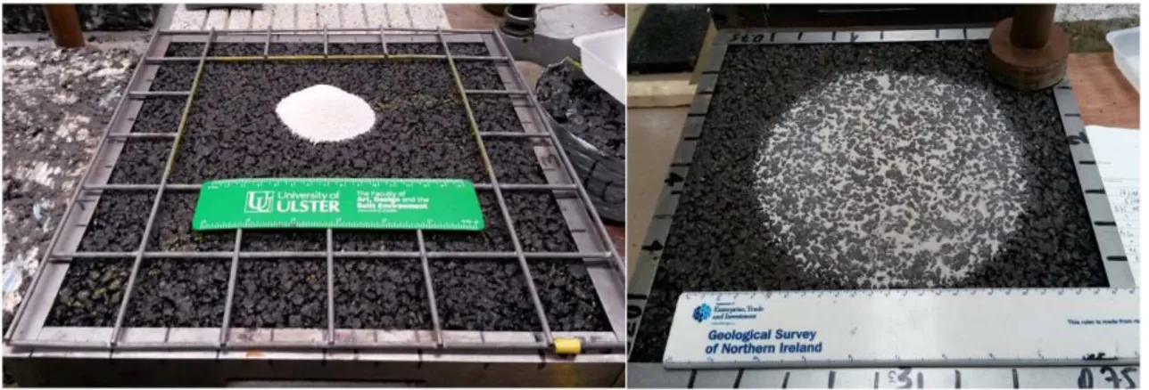
The sand patch or volumetric patch technique is used throughout the world to assess pavement surface macrotexture (EN 13036-1:2010). The method is used as the definitive assessment, or control value of a pavement surface materials macrotexture against which other measurement methods are compared. Despite this, it has limited use in research. The method relies on the spreading of a material, usually sand or glass spheres, in a patch. The material is distributed with a rubber pad to form an approximately circular patch, the average diameter of which is measured. By dividing the volume of material by the area covered, a value is obtained which represents the average depth of the layer, i.e. a 'mean texture depth'. The test gives a mean texture depth (MTD) value. Material properties such as aggregate size and shape are not indicated (EN 13036-1:2010) limiting its ability to fully assess surface texture.
7 EN 13036-3 (2002) details a method to determine the horizontal drainability of pavement surface texture. It is recommended for use only on smooth, low macrotexture non-porous surfaces. The method uses an outflow meter device and time as a measure of surface macrotexture. However the outflow meter provides minimum insight into the complexity of macrotexture. It gives little indication of any deterioration present in the surface, which may contribute to quicker outflow times than would be representative of the surface. The method has poor correlation with both MPD and MTD reflecting the different characteristics being assessed (McQuaid, 2015).
1.2.2 Non-contact
Laser based dynamic profilometers have been used for many years to measure pavement surface texture. These are typically vehicle mounted and use high-speed lasers. The measurements are either 2D profiles measured in the wheel path or 3D measurements of a lane width. The profiles produced by these devices can be used to compute various profile statistics, such as the Mean Profile Depth (MPD) and the Sensor Measured Texture Depth (SMTD).
Figure 1.3: Mean Profile Depth calculation
According to ISO 13473-1:1997, the MPD is calculated by dividing the measured profile into segments of 100 mm length (recommended base line). The slope of each segment is suppressed by subtracting a linear regression of the segment, providing a zero mean
8 profile. The MTD may be estimated through a conversion equation. In this case, the MTD is indicated as Estimated Texture Depth (ETD). Their relationship is:
= 0,2 + 0,8
An example of 2D wheel path measurement is the SCRIMTEX device. This is a WDM Sideway-force Coefficient Routine Investigation Machine (SCRIM) that measures both wet skid resistance and macrotexture in the same wheel path at either 30 or 60 mph. Development of technology and data processing has resulted in devices such as the Traffic Speed Condition Survey device (TRACS). This uses an array of lasers to measures macrotexture along with other data at highway speeds up to 60 miles per hour. This allows measurement of fretting, rut depth, estimates of surface type, cracking and sensor measured texture depth (SMTD).
The Pavemetrics Laser Crack Measuring System (LCMS) can produce transverse profiles of a road whilst travelling at speed. The LCMS consists of laser line projectors, filters and cameras. The device can scan a width of 4 m at a resolution of 1 mm. Identity data is used to allow interpretation of location. Features on the pavement surface such as rutting, cracks and line markings can be identified with a 95% certainty claimed (McQuaid, 2015). The Siteco Road-Scanner is a vehicle to carry out a rapid survey of a road infrastructure and combines the following technologies: GPS and Inertial Positioning System, medium-to-high resolution 5/8 front-mounted colour TV cameras and a rear-mounted vertical TV camera, a Dynatest RSPIV profilometer, a 2 GHz IDS georadar, an odometer and a Faro Photon 120 helical laser scanner. The latter acquires a cloud of laser points distributed on a helicoid at a step of 20-40 cm and lastly, the rear TV camera provides a continuous plane view of the road surface of around 4 m in width. Photogrammetric measurements are precise to 10 cm, while the relative accuracy obtained by the laser scanner (distance between 2 points) is of 2 mm (Lantieri et al., 2015).
The Circular Track Meter (CT meter) is an example of a static laser based non-contact method of road surface texture measurement (ASTM E2157, 2009). The CT meter is used in USA as a reference method of macrotexture measurement. The CT Meter uses a laser to measure the profile of a circle 284 mm in diameter or 892 mm in circumference. The profile is divided into eight segments of 111.5 mm and the average mean profile depth
9 (MPD) is determined for each of the segments of the circle. The reported MPD is the average of all eight segments depths. Several studies reported excellent correlations between the volumetric patch technique MTD and the CT Meter MPD. Among them Flintsch et al. (2003) regarded MPD as a two dimensional estimate of the three dimensional MTD.
1.3
Surface metrology on road pavements
Surface metrology is the science that deals with the characterization of a surface by the amplitude, spacing and shape of its features. One of the goal of this thesis is to understand the behaviour of asphalt mixtures that undergo simulated trafficking in terms of change of texture. This section will introduce key concepts that are at the base of the analysis presented in Chapter 8.
Figure 1.4 shows an example of a reconstructed 3D surface of an asphalt mixture. Even if it could appear a perfect representation of the real surface, it is not. In fact, it can be affected by roughness and waviness. Thus, two filters are defined: the S-filter and the L-filter- The first is defined as a filter that removes unwanted small-scale lateral components of the measured surface such as measurement noise or functionally irrelevant small features. The second is used to remove unwanted large-scale lateral components of the surface, and the F-operator removes the nominal form (by default using a least square method. The scale at which the filters operate is controlled by the nesting index, which is the extension of the notion of the original cut-off wavelength and is suitable for all types of filters. For example, for a Gaussian filter, the nesting index is equivalent to the cut-off wavelength. These filters are used in combination to create SF and SL surfaces. An SF surface results from using an S-filter and an F-operator in combination on a surface, and an SL surface by using an L-filter on an SF surface. Both are called scale-limited surface (Leach, 2010).
The scale-limited surface depends on the filters and operators used, with the scale being controlled by the nesting indices of those filters. The reference standard for the analysis of 3D areal surface texture is the ISO 25178. While defining all the parameters that will be presented hereafter, it always refers to the concept of scale-limited surface.
However scale-limited surfaces may display “fractal-type behaviours” over a range of scales.
10 A concept, which is essential and linked to any analysis, is the material ratio. The Material Ratio, mr, is the ratio of an intersecting area, parallel to the mean plane, passing through the surface at a given height to the cross sectional area of the evaluation region. The material ratio, according to Figure 1.5, is given by:
Figure 1.4: Reconstructed 3D surface of an asphalt sample
= ( + + + ) · 100
Figure 1.5: Concept of Material Ratio
The Areal Material Ratio Curve, referred to as the Abbot Firestone Curve, is established by evaluating mr at various levels from the highest peak to the lowest valley. Mathematically it represents the cumulative probability density function of the surface profile's height. An example of the AFC is shown in Figure 1.7. Using the Abbott curve,
11 a graphical study can be performed in order to retrieve functional parameters characterizing the profile, the surface or the volume intersected by a line or a plane. The equivalent straight line, calculated according to ISO 25178-2, intersects the 0 % and 100 % lines on the mr axis. From these points, two lines are plotted parallel to the x-axis; these determine the core surface by separating the protruding hills and dales. The vertical distance between these intersection lines is the material core. Their intersections with the areal material ratio curve define the material ratios Smr1 and Smr2. They are usually set at 10% and 80% respectively.
For one profile it is possible to extrapolate the parameters Rk, Rpk, and Rvk. They represent respectively the core roughness profile excluding the protruding peaks and the deep valleys, the average height of the protruding peaks above the core profile, and the average depth of the profile valleys projecting through the core profile. The parameters Rpk and Rvk are each calculated as the height of the right-angle triangle, which is constructed to have the same area as the “peak area” (A1) or “valley area” (A2), respectively.
Taking the previous concepts from one profile to one surface, the Abbott curve for the surface can be calculated. The reduced peak height, Spk, is a measure of the peak height above the core roughness. The core roughness Depth, Sk, is a measure of the “core” roughness (peak-to-valley) of the surface with the predominant peaks and valleys removed, according to the set thresholds. The reduced valley depth, Svk, is a measure of the valley depth below the core roughness.
Figure 1.6: Abbott curve for a single profile and parameters Rk, Rpk and Rvk (Bitelli et al., 2012)
12
Figure 1.7: Abbott curve for a surface and parameters Sk, Spk, Svk (Bitelli et al., 2012)
Following the identical procedure, the AFC can be calculated for the 3D surface, obtaining volume parameters:
Vv(mr), the Void Volume, is the volume of space bounded by the surface texture from a plane at a height corresponding to a chosen “mr” value to the lowest valley. “mr” may be set to any value from 0% to 100%.
Vvv(p), the Dale Void Volume, is the volume of space bounded by the surface texture from a plane at a height corresponding to a material ratio (mr) level, “p” to the lowest valley. The default value for “p” is 80% but may be changed as needed. Vvc(p,q), The Core Void Volume, is the volume of space bounded by the texture at heights corresponding to the material ratio values of “p” and “q”. The default value for “p” is 10% and the default value for “q” is 80%.
Vv(mr), Vvv(p) and Vvc(p,q) all indicate a measure of the void volume provided by the surface between various heights as established by the chosen material ratio(s) values. The volume parameters represents the more reliable way to study the change of surface texture. In this case, the y-axis is usually in terms of ml/m2.
1.4
Skid resistance
Friction between the tyre and road surface consists of two main components, both of which are related to speed:
a) adhesion between tyre and surface, which is a function of the microtexture, and depends on the nature of the materials in contact;
b) hysteresis, i.e. the loss of energy caused by tyre deformation, which is a function of the macrotexture.
13 Therefore, during a single braking operation the friction available to the vehicle is not constant.
In dry conditions all clean, surfaced roads have a high skidding resistance. In fact, when in a dry and clean state, roads generally provide insignificant differences in friction levels, regardless the type of pavement and surface configuration. On the other hand, the water acts as a lubrificant between the surface and the tyre, reducing friction.
The fine scale microtexture of the surface aggregate is the main contributor to sliding resistance and is the dominant factor in determining wet skidding resistance at lower speeds. Coarse Macrotexture, which provides rapid drainage routes between the tyre and road surface, and tyre resilience are important factors in determining wet skidding resistance at high speeds. Megatexture relates to the roughness of the road and has no effect on skidding resistance but affects noise (DMRB, 2006).
1.5
Measurement of skid resistance
Laboratory methods are used for evaluating the friction characteristics of core samples or laboratory-prepared samples. The two devices currently in use are the British Portable Tester (BPT), and the Japanese Dynamic Friction Tester (DFTester). The BPT will be discussed in a next Chapter as it was used for this thesis.
The Dynamic Friction Tester (DF Tester) is a portable instrument for measuring pavement surface friction as a function of speed and under various conditions. The instrument is comprised of a measuring unit and a control unit; an x-y plotter or laptop can be used to record data. The measuring unit consists of a disc made to rotate horizontally at a specified velocity before being lowered onto a wetted test surface for measurement of friction. The torque-generated by the resistance between the test surface and spring-loaded rubber "sliders" attached to the underside of the rotating disc is continuously monitored and converted to a measurement of friction.
Device % Slip (yaw angle)
Speed [km/h]
Country
British Portable Tester 100 10 United Kingdom
DFTester 100 0÷90 Japan
14 A summary of the devices for the friction measurement currently in use is presented in Table 1.3-1.6. There are four basic types of full-scale friction measuring devices depending on the slip condition of the measuring wheel: locked wheel, side force, fixed slip, and variable slip (NCHRP, 2000).
Locked wheel systems produce a 100 percent slip condition. The relative velocity between the surface of the tire and the pavement surface (the slip speed) is equal to the vehicle speed. The brake is applied and the force is measured and averaged for 1 second after the test wheel is fully locked. Because the force measurement is continuous during the braking process, these systems usually can detect the peak friction. The locked wheel testers are usually fitted with a self-watering system for wet testing, and a nominal water film of 0.5 mm is commonly used. When the measurement is made in accordance with ASTM Standard Test Method E-274 the result is reported as the skid number SN that is the measured value of friction times 100.
Device % Slip (yaw angle)
Speed
[km/h] Country
ASTM E-274 Trailer
100
30÷90 United States
Dagonal Braked Vehicle
(DBV) 65 United States
Japanese Skid Tester 30÷90 Japan
LCPC Adhera 40÷90 France
Polish SRT-3 30÷90 Japan
Skidclometer BV-8 30÷90 Sweden
Stuttgarter
Reibungsmesser (SRM) 100, 20 30÷90 Germany
Table 1.3: Locked Wheel friction measurement devices (NCHRP, 2000)
Side force systems maintain the test wheel in a plane at an angle (the yaw angle) to the direction of motion, otherwise the wheel is allowed to roll freely. The side force is measured perpendicular to the plane of rotation. An advantage of this method is that these devices can measure continuously through the test section, whereas locked wheel devices usually sample the friction over the distance corresponding to 1 second of the vehicle travel, after the brake is released.
15 These systems produce a low-speed measurement even though the vehicle velocity is high. Because these devices are low slip speed systems, they are sensitive to microtexture. For this reason, they are usually used in conjunction with a macrotexture measure. The most frequently used side force devices are the MuMeter and the SidewayForce Coefficient Routine lnvestigation Machine (SCRIM). Because they are relatively insensitive to variations in macrotexture most SCRIMs are now fitted with a laser macrotexture measurement system mounted on the front of the vehicle and are called SCRIMTEX.
Device % Slip (yaw angle) Speed [km/h] Country MuMeter 13 (7.5°) 20÷90 United Kingdom Odoliograph 34 (20°) 30÷90 Belgium SCRIM 34 (20°) 30÷90 United Kingdom Stradograph 21 (12°) 30÷90 Denmark
Table 1.4: Side Force friction measurement devices (NCHRP, 2000)
Fixed Slip devices operate at a constant slip, usually between 10 and 20 percent. The test wheel is driven at a lower angular velocity than its free rolling velocity. This is usually accomplished by incorporating a gear reduction or chain drive of the test wheel drive shaft from the drive shaft of the host vehicle. In some cases, it is accomplished by hydraulic retardation of the test wheel. These devices also measure low-speed friction as the slip speed is V (% slip/100).
Device % Slip (yaw angle) Speed [km/h]
Country
DWW Trailer 86 30÷90 Netherlands
Griptester 14.5 30÷90 United Kingdom
Runway Frïction tester 15 30÷90 United States
Saab Friction Tester 15 30÷90 Sweden
Skiddometer BV-l I 20 30÷90 Sweden
16 Like the side force method, the fixed slip method can also be operated continuously over the test section without excessive wear of the test tyre.
An example of a fixed slip tester is the Griptester. Most fixed slip devices are designed to operate at only one slip ratio; however the slip ratio can be varied on some fixed slip devices, referred to as variable fixed slip devices.
Variable slip devices sweep through a predetermined set of slip ratios. This is usually accomplished by driving the test wheel through a programmed slip ratio using a hydraulic motor. Some locked wheel testers can be operated in a mode that captures the friction as the test tire proceeds from free rolling to the fully locked wheel condition (0 to 100 percent slip). Locked wheel testers can also be programmed to operate in acccordance with ASTM E1337, in which the brake is released just after the peak is reached (NCHRP, 2000).
Device % Slip (yaw angle) Speed [km/h] Country IMAG 0÷100 30÷90 France
Komatsu Skid Tester 10÷30 30÷60 Japan Norsemeter Oscar 0÷90 30÷90 Norway
Norsemetel ROAR 0÷90 30÷90 Norway
Norsemeter SAUIAR 0÷90 30÷90 Norway
Table 1.6: Variable - Fixed slip friction measurement devices (NCHRP, 2000)
1.6PIARC harmonization – IFI index
Due to the great variety of measurement devices, the World Road Association - PIARC carried out an International experiment to compare and harmonize texture and skid resistance measurements in the fall of 1992. There were 51 different friction and texture measurements made by participants from 14 countries. The measurements were conducted on 54 sites as follows: 28 sites in Belgium (22 on public roads, 2 at airports, and 4 at racetracks) and 26 sites in Spain (18 on public roads and 8 at airports). Texture measurements, and friction measurements. Each friction tester was operated at three speeds: 30, 60 and 90 km/h, and each tester made two repeated runs at each speed. All texture measurements were made on dry surfaces before any water was applied to the roadway. As a control, a microtexture measurement was made before and after the skid
17 testers made their tests. These data were used to show that there were no statistically significant changes occurring during the testing.
Since the aim of the Technical Committee of the Surface characteristics AIRPC was to harmonize the different measurement methods used for the evaluation of friction and texture of road surfaces, a single index was proposed. The IFI index (International Friction Index) is calculated using relationships obtained from regressions of friction and textural data detected with different types of equipment.
= ( ; !")
Where:
!" is the speed constant in km/h. It does not depend on the adopted equipment for the
friction measurement and it is function of the Mean Profile Depth only. It is calculated as follows.
!" = + # ·
The coefficients a and b depend on the equipment adopted for the measure of macrotexture.
is the parameter that represents the friction at the reference speed of 60 km/h and it is calculated as follows.
= + · $ + ·
The coefficients A, B and C depend on the type of instrument used for the measurement of the friction, while $ is the friction coefficient measured by the adopted instrument at the sliding speed of 60 km/h, which is calculated as follows.
= $%· exp )! − 60! " ,
$% is the friction coefficient measured at the sliding speed S of the adopted equipment, which is calculated as follows.
18 In this case, V is the measurement cart speed in km/h while s is the sliding of the measurement wheel.
A, B, and C were determined were tabulated in the ASTM Standard Practice E-1960. The value of C is always zero when the friction is measured with a smooth tread tire. However, the term · was found to be necessary for ribbed or patterned test tires because they are relatively insensitive to macrotexture.
The two parameters that make up the IFI / ; !"0 are sufficient to describe the friction as a function of slip speed. Note that a texture measurement is required to apply the IFI. Another advantage of the IFI is that the value of for a pavement will be the same regardless of the slip speed. That permits the test vehicle to operate at any safe speed that could be at higher speeds on high-speed highways and lower speeds in urban situations.
19
Literature review
2.1
Texture
The texture of laboratory test specimens has traditionally been measured using the volumetric patch technique as used for pavement surfacing. This allows direct comparison of road and laboratory data. However, research has considered complimentary non-contact alternatives to better understand the role of texture at different scales (McQuaid, 2015). Among them Millar (2013) compared the use of a 3D hand held laser and close range photogrammetry (CRP) techniques and analyzed the models using functional volume parameters.
Flintsch et al. (2003) discussed different techniques for measuring pavement surface macrotexture and its application in pavement management and investigated a series of correlations between different measuring devices through the survey of many wearing surfaces.
Sangiorgi et al (2013) used a laser laboratory device to collect point cloud data for a section of road surfaces and used a combination of roughness parameters, MPD and Abbott-Firestone Curve analysis techniques.
Friel (2013), Mitchell (2014) and McQuaid (2015) used the Close Range Photogrammetry method and a hand held 3D laser respectively to assess surface texture changes with time for asphalt test specimens subject to accelerated simulated trafficking with the Road Test Machine.
Losa et al. (2010) looked for a reliable pavement profile data processing procedure for evaluation of pavement macrotexture, according to the definition of the ISO 13473-1, and for the verification of the assumption of equivalence between the profilometric and volumetric methods.
20 2.1.1 A comparison of techniques to determine surface texture data
This paper investigates the 3D capture of specimen surface texture using both Close Range Photogrammetry and High Resolution Scanner (HRS) methodologies. A vinyl cast with vinamold was made and assessed. The vinyl cast technique results in a permanent record of the asphalt surface texture and allows for time based studies showing its evolution. The 3D meshes were analysed for a 2D and 3D areal parameters using Digital Surf MountainsMap 6. Analysis of the findings show how sand patch, 3D photogrammetry and laser techniques data may be used to better understand road surface textures.
The analysis was made on a laboratory compacted hot rolled asphalt (HRA) test specimen. This was 305 x 305 x 50 mm in size and had Silurian greywacke 20 mm chippings at a spread rate 12 kg/m² applied during compaction to create macrotexture. The test specimen underwent 10,000 wheel passes of accelerated wet trafficking on the University of Ulster Road Test Machine (RTM).
The CRP procedure used a Canon EOS 400D SLR camera, with a 10Mp CCD array and a calibrated 60 mm macro lens. All images were captured normal to the surface under natural lighting conditions. The camera was mounted on a tripod and a remote shutter release used to minimize camera shake. A framework of control points was used to allow the recovery of surface elevation and orientation. It was calibrated using a digital micrometer forming a control calibration file. The control points were cross matched with additional tie points to reduce the level of redundancy. The stereo image pair, control calibration file and camera calibration files were imported into Topcon ImageMaster photogrammetric software. A TIN was created at a mesh resolution of 0.5 mm. No filtering was applied to the TIN in case it removed surface roughness. The resultant Cartesian coordinates of the TIN were exported in a comma separated value (CSV) file format into Digital Surf MountainsMap Version 6 surface analysis software.
The HRS procedure used a ZScanner 800 high resolution 3D laser scanner (HRS) with a stated resolution of 50 μm. A combination of scan resolutions was used to maximize the point cloud for the test specimen surface. This involved an initial coarse scan at 2 mm resolution followed by a fine resolution scan of 0.5 mm. Figure 2 shows the reference framework of control points used during laser scanning. After scanning and prior to export, the point cloud facets were edited to remove redundant data points. The facet resolution was set to 0.5 mm, allowing a comparable 3D model with that produced though
21 the CRP procedure. The point cloud was exported as a TXT file into Digital Surf MountainsMap Version6 surface analysis software. Digital Surf MountainsMap software allowed 2D and 3D parameters to be measured in accordance with BS EN ISO 25178-2. The Study concluded that:
• The height parameters, Sq, Sa, Sp and Sv showed consistently higher values for the use of the cast compared to the slab. The same relationship occurs when the CRP method is compared with the HRS. The Ssk and Sku values correlated well with each other for all four 3D models. This suggests that the use of the cast for 3D capture of surface texture recovered to a greater depth into the surface when compared with the slab 3D models • The AFC and percentage depth distribution data was able to confirm the presence of surface noise in CRP derived 3D models. As with previous SMA analysis this had negligible effect on the volumetric analysis (AFC) but did influence the height parameters. • The removal of 1% AMBR to the peaks and valleys (AMBR 1% - 99%) can be used to remove outlier data due.
2.1.2 A study on texture and acoustic properties of cold laid microsurfacings This study aim was to develop a slurry seal microsurfacings, which, in addition to skid resistance and roughness characteristics, would provide rolling noise reduction and eco-compatibility characteristics with the use of recycled crumb rubber. A 3D laser scanner device has been used to evaluate the surface texture and analyze the roughness parameters. Goals are similar to those reached by this PhD thesis.
Various bituminous mixtures for cold microsurfacings have been tested in laboratory conditions: they contained porphyry and basalt aggregates and a fraction of crumb rubber equal to 1.5 % on the mixture weight. Then, they were mixed with Portland cement, water and 60% bitumen emulsion modified with latex.
After the definition of the gradation curves by determining the best dosage of the compounds, four mixtures have been selected for the in-situ application: one with only basaltic aggregates (KmodBB), one with basaltic sand and porphyritic aggregate (KmodBP) and the same two mixtures, where a part of the sand fraction has been replaced by crumb rubber (KmodBBp and KmodBPp).
22 After the microsurfacings have been laid, a series of in situ surveys was carried out to characterize the road surface texture by means of a high-precision laser scanner device. The system used in this work is produced by the NextEngine and is based on the Multi-stripe Laser Triangulation (MLT) technology (Desktop 3D), capable of recording the three-dimensional representation of the surface texture of a portion of pavement.
The BPN and HS tests were performed in 10 longitudinally-equidistant road sections for both directions, in order to cover the whole road stretch, while two road areas per lane close to the Sound Level Meter have been laser scanned.
According to ISO 13473-2, 2D and 3D parameters were calculated for two of the three analyzed sites. An interesting study was represented by the correlation between the emerged area and water volume retention. The same study will be presented later for the rubberized 8 mm SMA in the 3D Image analysis Chapter. Sangiorgi et al. found a higher percentage of emerged areas in basaltic mixtures, instead of the basaltic and porphyritic ones, stating that this results is linked to the greater roughness of the surface. According to the ISO 25178 other indicators were calculated, i.e. areal and volumetric parameters, for a better classification of the pavement texture components (peaks, valleys and the core roughness profile) through the construction of the Abbott curves. Bearing ratio thresholds were set by default to 10% and 80%. Volume of material peak was found to be around 30 ml/m2 and volume of void ranged between 66.30 and 84.30 ml/m2.
As for the acoustic measurements, the Statistical Pass-By Method (UNI EN ISO 11819-1) was chosen, for its reliability and representativeness of the actual perception of road noise by receptors located close to the transportation infrastructure and it was applied on a statistically significant sample of passing-by road vehicles. Results highlighted a reduction equal to 2.2 dB(A) in the first site for the KmodBBp surface, compared to the previous asphalt pavement, while for the KmodBB one the reduction was equal to 0.7 dB(A).
In the second site the tests returned more similar results for both KmodBP and KmodBPp mixtures, with a reduction respectively equal to 1.5 dB(A) and 1.6 dB(A). In the third site, the A-weighted sound pressure levels related to one of the vehicle categories, did not undergone significant modifications and, therefore, the SPBI indexes remain substantially unaltered.
23 The paper concludes with the announce of new experimental and trial sites with the aim of the study the relationship between geometric and statistical indicators of a road surface texture and its noise performances: this PhD thesis confirms this statement.
2.1.3 Changes of surface dressing texture as related to time and chipping size This paper reports the findings of a research project to study surface dressing performance in terms of its aggregate embedment due to trafficking and of the skid resistance and texture depth change with time. The influence of chipping size is also discussed. The reference materials are a range of smaller chipping sizes embedded into three types of underlying surfaces i.e. soft sand asphalt, 14mm Stone Mastic Asphalt (SMA) and concrete. The test specimens were compacted using a 17kg hand roller compacter with a minimum of 10 passes until the chippings were laid on their least dimension. Each test specimen was kept in an oven at 200°C for 24 hours to remove the water present in the emulsion. The rate of spread of binder and chippings was in accordance to Road Note 39. The wheel-tracker equipment was used to simulate trafficking of a small scale pavement structure and test for chipping embedment into the underlying material. Testing was periodically stopped and changes in texture depth and dry skid resistance determined. The authors divided the data into three stages. The first stage lasted for approximately 1960 passes of wheel tracking, followed by a second stage of between 1950 to 6240 passes. After 6240 passes, the test specimen was considered as belonging to a third stage where the rate of chipping embedment becomes minimal. The discussion of results is divided into three parts, dealing with texture depth, skid resistance and both of them respectively. As for the texture depth, results showed that as the tracking time increased texture depth decreased at a gradually rate. Embedment was rapid during the initial stages after which the rate slows down which is expected as the chippings become interlocked.
The development of early life dry skid resistance was not as predictable as the decay in texture depth. This was attributed to complex interactions linked to the aggregate particles re-orientation, the embedding and polishing during prolonged tracking. This appeared to cause an initial increase in skid resistance followed by a gradual reduction. Skid resistance attains a maximum value soon after construction, when all the asphalt film on the surface has been worn away and the fresh gritty surface of the aggregate is exposed. With time,

![Figure 3.3: Designed and sampled grading curves 010203040506070809010002468 10 12% Sieve passingSieve [mm]SMA desSMA laidSMA 0.75 desSMA 0.75 laidSMA 1.20 desSMA 1.20 laid](https://thumb-eu.123doks.com/thumbv2/123dokorg/8136129.125958/91.892.212.695.779.1107/figure-designed-sampled-grading-curves-passingsieve-laidsma-laidsma.webp)