Observation of J=ψp Resonances Consistent with Pentaquark States
in Λ
0b
→ J=ψK
−p Decays
R. Aaij et al.*
(LHCb Collaboration)
(Received 13 July 2015; published 12 August 2015)
Observations of exotic structures in the J=ψp channel, which we refer to as charmonium-pentaquark states, in Λ0
b→ J=ψK−p decays are presented. The data sample corresponds to an integrated luminosity of
3 fb−1 acquired with the LHCb detector from 7 and 8 TeV pp collisions. An amplitude analysis of the three-body final state reproduces the two-body mass and angular distributions. To obtain a satisfactory fit of the structures seen in the J=ψp mass spectrum, it is necessary to include two Breit-Wigner amplitudes that each describe a resonant state. The significance of each of these resonances is more than 9 standard deviations. One has a mass of 4380 ! 8 ! 29 MeV and a width of 205 ! 18 ! 86 MeV, while the second is narrower, with a mass of 4449.8 ! 1.7 ! 2.5 MeV and a width of 39 ! 5 ! 19 MeV. The preferred JP
assignments are of opposite parity, with one state having spin 3=2 and the other 5=2.
DOI:10.1103/PhysRevLett.115.072001 PACS numbers: 14.40.Pq, 13.25.Gv
Introduction and summary.—The prospect of hadrons with more than the minimal quark content (q¯q or qqq) was proposed by Gell-Mann in 1964 [1] and Zweig [2], followed by a quantitative model for two quarks plus two antiquarks developed by Jaffe in 1976[3]. The idea was expanded upon [4]to include baryons composed of four quarks plus one antiquark; the name pentaquark was coined by Lipkin[5]. Past claimed observations of penta-quark states have been shown to be spurious[6], although there is at least one viable tetraquark candidate, the Zð4430Þþobserved in ¯B0→ ψ0K−πþdecays[7–9],
imply-ing that the existence of pentaquark baryon states would not be surprising. States that decay into charmonium may have particularly distinctive signatures[10].
Large yields of Λ0
b→ J=ψK−p decays are available at
LHCb and have been used for the precise measurement of the Λ0
blifetime[11]. (In this Letter, mention of a particular
mode implies use of its charge conjugate as well.) This decay can proceed by the diagram shown in Fig.1(a), and is expected to be dominated by Λ%→ K−p resonances, as are
evident in our data shown in Fig.2(a). It could also have exotic contributions, as indicated by the diagram in Fig. 1(b), which could result in resonant structures in the J=ψp mass spectrum shown in Fig.2(b).
In practice, resonances decaying strongly into J=ψp must have a minimal quark content of c¯cuud, and thus are charmonium pentaquarks; we label such states Pþc,
irre-spective of the internal binding mechanism. In order to
ascertain if the structures seen in Fig.2(b)are resonant in nature and not due to reflections generated by the Λ%states,
it is necessary to perform a full amplitude analysis, allowing for interference effects between both decay sequences.
The fit uses five decay angles and the K−p invariant
mass mKpas independent variables. First, we tried to fit the data with an amplitude model that contains 14 Λ% states
listed by the Particle Data Group[12]. As this did not give a satisfactory description of the data, we added one Pþc state,
and when that was not sufficient we included a second state. The two Pþc states are found to have masses of
4380! 8 ! 29 MeV and 4449.8 ! 1.7 ! 2.5 MeV, with corresponding widths of 205 ! 18 ! 86 MeV and 39! 5 ! 19 MeV. (Natural units are used throughout this Letter. Whenever two uncertainties are quoted, the first is statistical and the second systematic.) The fractions of the total sample due to the lower mass and higher mass states are ð8.4 ! 0.7 ! 4.2Þ% and ð4.1 ! 0.5 ! 1.1Þ%, respec-tively. The best fit solution has spin-parity JP values of
(3=2−, 5=2þ). Acceptable solutions are also found for
additional cases with opposite parity, either (3=2þ, 5=2−) or
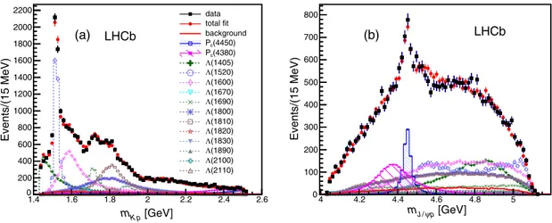
(5=2þ, 3=2−). The best fit projections are shown in Fig.3.
Both mKp and the peaking structure in mJ=ψp are repro-duced by the fit. The significances of the lower mass and
(a) (b)
FIG. 1 (color online). Feynman diagrams for (a) Λ0
b→ J=ψΛ%
and (b) Λ0
b→ PþcK−decay. *Full author list given at end of the article.
Published by the American Physical Society under the terms of theCreative Commons Attribution 3.0 License. Further distri-bution of this work must maintain attridistri-bution to the author(s) and the published article’s title, journal citation, and DOI.
higher mass states are 9 and 12 standard deviations, respectively.
Analysis and results.—We use data corresponding to 1 fb−1 of integrated luminosity acquired by the LHCb experiment in pp collisions at 7 TeV center-of-mass energy, and 2 fb−1 at 8 TeV. The LHCb detector [13]
is a single-arm forward spectrometer covering the pseudorapidity range, 2 < η < 5. The detector includes a high-precision tracking system consisting of a silicon-strip vertex detector surrounding the pp interaction region[14], a large-area silicon-strip detector located upstream of a dipole magnet with a bending power of about 4 Tm, and three stations of silicon-strip detectors and straw drift tubes
[15]placed downstream of the magnet. Different types of charged hadrons are distinguished using information from two ring-imaging Cherenkov detectors [16]. Muons are identified by a system composed of alternating layers of iron and multiwire proportional chambers[17].
Events are triggered by a J=ψ → μþμ−decay, requiring
two identified muons with opposite charge, each with transverse momentum, pT, greater than 500 MeV. The
dimuon system is required to form a vertex with a fit χ2 < 16, to be significantly displaced from the nearest pp
interaction vertex, and to have an invariant mass within 120 MeV of the J=ψ mass [12]. After applying these requirements, there is a large J=ψ signal over a small background[18]. Only candidates with dimuon invariant mass between−48 and þ43 MeV relative to the observed J=ψ mass peak are selected, the asymmetry accounting for final-state electromagnetic radiation.
Analysis preselection requirements are imposed prior to using a gradient boosted decision tree, BDTG [19], that separates the Λ0
b signal from backgrounds. Each track is
required to be of good quality and multiple reconstructions of the same track are removed. Requirements on the individual particles include pT > 550 MeV for muons,
[GeV] p K m 1.4 1.6 1.8 2.0 2.2 2.4 Events/(20 MeV) 500 1000 1500 2000 2500 3000 LHCb (a) data phase space [GeV] p ψ / J m 4.0 4.2 4.4 4.6 4.8 5.0 Events/(15 MeV) 200 400 600 800 (b) LHCb
FIG. 2 (color online). Invariant mass of (a) K−p and (b) J=ψp combinations from Λ0
b→ J=ψK−p decays. The solid (red) curve is the
expectation from phase space. The background has been subtracted.
[GeV] p K m 1.4 1.6 1.8 2 2.2 2.4 2.6 Events/(15 MeV) 0 200 400 600 800 1000 1200 1400 1600 1800 2000 2200 LHCb data total fit background (4450) c P (4380) c P (1405) Λ (1520) Λ (1600) Λ (1670) Λ (1690) Λ (1800) Λ (1810) Λ (1820) Λ (1830) Λ (1890) Λ (2100) Λ (2110) Λ [GeV] p ψ / J m 4 4.2 4.4 4.6 4.8 5 Events/(15 MeV) 0 100 200 300 400 500 600 700 800 LHCb (a) (b)
FIG. 3 (color online). Fit projections for (a) mKpand (b) mJ=ψpfor the reduced Λ%model with two Pþc states (see TableI). The data are
shown as solid (black) squares, while the solid (red) points show the results of the fit. The solid (red) histogram shows the background distribution. The (blue) open squares with the shaded histogram represent the Pcð4450Þþ state, and the shaded histogram topped with
(purple) filled squares represents the Pcð4380Þþstate. Each Λ%component is also shown. The error bars on the points showing the fit
and pT> 250 MeV for hadrons. Each hadron must have an
impact parameter χ2 with respect to the primary pp
interaction vertex larger than 9, and must be positively identified in the particle identification system. The K−p
system must form a vertex with χ2< 16, as must the two
muons from the J=ψ decay. Requirements on the Λ0 b
candidate include a vertex χ2 < 50 for 5 degrees of
free-dom, and a flight distance of greater than 1.5 mm. The vector from the primary vertex to the Λ0
bvertex must align
with the Λ0
b momentum so that the cosine of the angle
between them is larger than 0.999. Candidate μþμ−
combinations are constrained to the J=ψ mass for sub-sequent use in event selection.
The BDTG technique involves a “training” procedure using sideband data background and simulated signal samples. (The variables used are listed in the Supplemental Material [20].) We use 2 × 10⁶ Λ0
b→
J=ψK−p events with J=ψ → μþμ− that are generated
uniformly in phase space in the LHCb acceptance, using
PYTHIA[21]with a special LHCb parameter tune[22], and
the LHCb detector simulation based on GEANT4 [23], described in Ref.[24]. The product of the reconstruction and trigger efficiencies within the LHCb geometric accep-tance is about 10%. In addition, specific backgrounds from
¯ B0
s and ¯B0 decays are vetoed. This is accomplished by
removing combinations that when interpreted as J=ψKþK−
fall within !30 MeV of the ¯B0
smass or when interpreted as
J=ψK−πþ fall within !30 MeV of the ¯B0 mass. This
requirement effectively eliminates background from these sources and causes only smooth changes in the detection efficiencies across the Λ0
bdecay phase space. Backgrounds
from Ξb decays cannot contribute significantly to our
sample. We choose a relatively tight cut on the BDTG output variable that leaves 26 007 ! 166 signal candidates containing 5.4% background within !15 MeV (!2σ) of the J=ψK−p mass peak, as determined by the unbinned
extended likelihood fit shown in Fig.4. The combinatorial background is modeled with an exponential function and the Λ0
b signal shape is parametrized by a double-sided
Hypatia function [25], where the signal radiative tail parameters are fixed to values obtained from simulation. For subsequent analysis we constrain the J=ψK−p
four-vectors to give the Λ0
binvariant mass and the Λ0bmomentum
vector to be aligned with the measured direction from the primary to the Λ0
b vertices[26].
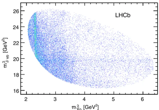
In Fig.5we show the “Dalitz” plot[27]using the K−p
and J=ψp invariant masses-squared as independent vari-ables. A distinct vertical band is observed in the K−p
invariant mass distribution near 2.3 GeV2corresponding to
the Λð1520Þ resonance. There is also a distinct horizontal band near 19.5 GeV2. As we see structures in both K−p
and J=ψp mass distributions we perform a full amplitude analysis, using the available angular variables in addition to the mass distributions, in order to determine the
resonances present. No structure is seen in the J=ψK−
invariant mass.
We consider the two interfering processes shown in Fig. 1, which produce two distinct decay sequences: Λ0
b→ J=ψΛ%, Λ%→ K−p and Λb0 → PþcK−, Pþc → J=ψp,
with J=ψ → μþμ− in both cases. We use the helicity
formalism [28] in which each sequential decay A → BC contributes to the amplitude a term
HA→BC λB;λC D JA λA;λB−λCðϕB; θA; 0Þ%RAðmBCÞ ¼ HA→BCλB;λC e iλAϕBdJA λA;λB−λCðθAÞRAðmBCÞ; ð1Þ
where λ is the quantum number related to the projection of the spin of the particle onto its momentum vector (helicity) and HA→BC
λB;λC are complex helicity-coupling amplitudes
describing the decay dynamics. Here, θA and ϕB are the
polar and azimuthal angles of B in the rest frame of A (θAis
known as the “helicity angle” of A). The three arguments of Wigner’s D matrix are Euler angles describing the rotation of the initial coordinate system with the z axis along the
[MeV] 5500 5600 5700 Events / ( 4 MeV) 0 1000 2000 3000 4000 5000 6000 7000 LHCb p ψ / J m K
FIG. 4 (color online). Invariant mass spectrum of J=ψK−p
combinations, with the total fit, signal, and background compo-nents shown as solid (blue), solid (red), and dashed lines, respectively. ] 2 [GeV Kp 2 m 2 3 4 5 6 ] 2 [GeVp ψ J/ 2 m 16 18 20 22 24 26 LHCb
FIG. 5 (color online). Invariant mass squared of K−p versus
J=ψp for candidates within !15 MeV of the Λ0 b mass.
helicity axis of A to the coordinate system with the z axis along the helicity axis of B[12]. We choose the convention in which the third Euler angle is zero. In Eq. (1), dJA
λA;λB−λCðθAÞ is the Wigner small-d matrix. If A has a
non-negligible natural width, the invariant mass distribu-tion of the B and C daughters is described by the complex function RAðmBCÞ discussed below; otherwise
RAðmBCÞ ¼ 1.
Using Clebsch-Gordan coefficients, we express the helicity couplings in terms of LS couplings (BL;S), where
L is the orbital angular momentum in the decay, and S is the total spin of A plus B:
HA→BC λB;λC ¼ X L X S ffiffiffiffiffiffiffiffiffiffiffiffiffiffiffi 2Lþ1 2JAþ1 s BL;S"JB JC S λB −λC λB−λC # ×"L S JA 0 λB−λC λB−λC # ; ð2Þ
where the expressions in parentheses are the standard Wigner 3j symbols. For strong decays, possible L values are constrained by the conservation of parity (P): PA¼ PBPCð−1ÞL.
Denoting J=ψ as ψ, the matrix element for the Λ0 b→ J=ψΛ% decay sequence is MΛ% λΛ0 b;λp;Δλμ ≡X n X λΛ% X λψ HΛ0b→Λ%nψ λΛ%;λψ D 1=2 λΛ0 b;λ % Λ−λψð0; θΛ0b; 0Þ % × HΛ%n→Kp λp;0 D JΛ%n λΛ%;λpðϕK; θΛ%; 0Þ%RΛ%nðmKpÞ × D1 λψ;Δλμðϕμ; θψ; 0Þ%; ð3Þ
where the x axis, in the coordinates describing the Λ0 b
decay, is chosen to fix ϕΛ% ¼ 0. The sum over n is due to
many different Λ%n resonances contributing to the
ampli-tude. Since the J=ψ decay is electromagnetic, the values of Δλμ≡ λμþ− λμ− are restricted to !1.
There are four (six) independent complex HΛ0b→Λ%nψ
λΛ%;λψ
couplings to fit for each Λ%n resonance for JΛ%
n¼
1 2 (>
1 2).
They can be reduced to only one (three) free BL;Scoupling
to fit if only the lowest (the lowest two) values of L are considered. The mass mKp, together with all decay angles
entering Eq. (3), θΛ0
b, θΛ%, ϕK, θψ, and ϕμ (denoted
collectively as Ω), constitute the six independent dimen-sions of the Λ0
b→ J=ψpK− decay phase space.
Similarly, the matrix element for the Pþc decay chain is
given by MPc λΛ0 b;λ Pc p;ΔλPcμ ≡X j X λPc X λPcψ HΛ0b→PcjK λPc;0 D1=2λΛ0 b;λPcðϕ Pc; θ Pc Λ0 b; 0Þ % × HPcj→ψp λPcψ ;λPcp D JPcj λPc;λPcψ −λPcp ðϕψ; θPc; 0Þ %RP cjðmψpÞ × D1 λPcψ ;ΔλPcμ ðϕ Pc μ ; θPψc; 0Þ%; ð4Þ
where the angles and helicity states carry the superscript or subscript Pcto distinguish them from those defined for the Λ%decay chain. The sum over j allows for the possibility of
contributions from more than one Pþc resonance. There are
two (three) independent helicity couplings HPcj→ψp
λPcψ ;λPcp for
JPcj¼
1 2(>
1
2), and a ratio of the two H Λ0
b→PcjK
λPc;0 couplings,
to determine from the data.
The mass-dependent RΛ%nðmKpÞ and RPcjðmJ=ψpÞ terms
are given by RXðmÞ ¼ B0LX Λ0bðp; p0; dÞ " p MΛ0 b #LX Λ0b × BWðmjM0X;Γ0XÞB0LXðq; q0; dÞ " q M0X #LX : ð5Þ Here p is the X ¼ Λ% or Pþc momentum in the Λ0
b rest
frame, and q is the momentum of either decay product of X in the X rest frame. The symbols p0and q0denote values of these quantities at the resonance peak (m ¼ M0X). The
orbital angular momentum between the decay products of Λ0
b is denoted as LXΛ0
b. Similarly, LX is the orbital angular
momentum between the decay products of X. The orbital angular momentum barrier factors, pLB0
Lðp; p0; dÞ, involve
the Blatt-Weisskopf functions [29], and account for the difficulty in creating larger orbital angular momentum L, which depends on the momentum of the decay products p and on the size of the decaying particle, given by the d constant. We set d ¼ 3.0 GeV−1∼ 0.6 fm. The relativistic
Breit-Wigner amplitude is given by BWðmjM0X;Γ0XÞ ¼ 1 M0X2− m2− iM0XΓðmÞ ; ð6Þ where ΓðmÞ ¼ Γ0X " q q0 #2LXþ1M 0X m B0LXðq; q0; dÞ 2 ð7Þ
is the mass-dependent width of the resonance. For the Λð1405Þ resonance, which peaks below the K−p threshold,
(see the Supplemental Material[20]). The couplings for the allowed channels,Σπ and Kp, are taken to be equal and to correspond to the nominal value of the width[12]. For all resonances we assume minimal values of LX
Λ0
b and of LXin
RXðmÞ. For nonresonant (NR) terms we set BWðmÞ ¼ 1
and M0NR to the midrange mass.
Before the matrix elements for the two decay sequences can be added coherently, the proton and muon helicity states in the Λ% decay chain must be expressed in the basis
of helicities in the Pþc decay chain,
jMj2 ¼X λΛ0 b X λp X Δλμ $ $ $ $MΛλΛ0% b;λp;Δλμ þ eiΔλμαμX λPcp d1=2 λPcp;λpðθpÞM Pc λΛ0 b;λ Pc p;Δλμ $ $ $ $ 2 ; ð8Þ
where θpis the polar angle in the p rest frame between the
boost directions from the Λ%and Pþc rest frames, and αμis
the azimuthal angle correcting for the difference between the muon helicity states in the two decay chains. Note that mψp, θPΛbc, ϕPc, θPc, ϕψ, θ
Pc
ψ , ϕPμc, θp, and αμ can all be
derived from the values of mKp and Ω, and thus do not constitute independent dimensions in the Λ0
b decay phase
space. (A detailed prescription for calculation of all the angles entering the matrix element is given in the Supplemental Material[20].)
Strong interactions, which dominate Λ0
bproduction at the
LHC, conserve parity and cannot produce longitudinal Λ0 b
polarization[31]. Therefore, λΛ0
b ¼ þ1=2 and −1=2 values
are equally likely, which is reflected in Eq.(8). If we allow the Λ0
b polarization to vary, the data are consistent with a
polarization of zero. Interferences between various Λ%nand
Pþ
cj resonances vanish in the integrated rates unless the
resonances belong to the same decay chain and have the same quantum numbers.
The matrix element given by Eq.(8)is a six-dimensional function of mKpandΩ and depends on the fit parameters,
~ω, which represent independent helicity or LS couplings, and masses and widths of resonances (or Flatté parameters), M ¼ MðmKp;Ωj~ωÞ. After accounting for the selection
efficiency to obtain the signal probability density function (PDF), an unbinned maximum likelihood fit is used to determine the amplitudes. Since the efficiency does not depend on ~ω, it is needed only in the normalization integral, which is carried out numerically by summing jMðmKp;Ωj~ωÞj2 over the simulated events generated
uniformly in phase space and passed through the selection. (More details are given in the Supplemental Material[20].) We use two fit algorithms, which were independently coded and which differ in the approach used for back-ground subtraction. In the first approach, which we refer to
as cFit, the signal region is defined as !2σ around the Λ0 b
mass peak. The total PDF used in the fit to the candidates in the signal region, PðmKp;Ωj~ωÞ, includes a background
component with normalization fixed to be 5.4% of the total. The background PDF is found to factorize into five two-dimensional functions of mKp and of each independent
angle, which are estimated using sidebands extending from 5.0σ to 13.5σ on both sides of the peak.
In the complementary approach, called sFit, no explicit background parametrization is needed. The PDF consists of only the signal component, with the background subtracted using the sPlot technique[32]applied to the log-likelihood sum. All candidates shown in Fig.4are included in the sum with weights, Wi, dependent on mJ=ψKp. The weights are set according to the signal and the background probabilities determined by the fits to the mJ=ψpKdistributions, similar to
the fit displayed in Fig.4, but performed in 32 different bins of the two-dimensional plane of cos θΛ0
b and cos θJ=ψ to
account for correlations with the mass shapes of the signal and background components. This quasi-log-likelihood sum is scaled by a constant factor, sW≡PiWi=PiWi2,
to account for the effect of the background subtraction on the statistical uncertainty. (More details on the cFit and sFit procedures are given in the Supplemental Material[20].)
In each approach, we minimize −2 ln Lð~ωÞ ¼ −2sWPiWiln PðmKpi;Ωij~ωÞ, which gives the estimated
values of the fit parameters, ~ωmin, together with their covariance matrix (Wi ¼ 1 in cFit). The difference of
−2 ln Lð~ωminÞ between different amplitude models,
Δð−2 ln LÞ, allows their discrimination. For two models representing separate hypotheses, e.g., when discriminating between different JP values assigned to a Pþ
c state, the
assumption of a χ2distribution with 1 degree of freedom for
Δð−2 ln LÞ under the disfavored JP hypothesis allows the
calculation of a lower limit on the significance of its rejection, i.e., the p value[33]. Therefore, it is convenient to expressΔð−2 ln LÞ values as n2
σ, where nσ corresponds
to the number of standard deviations in the normal distribution with the same p value. For nested hypotheses, e.g., when discriminating between models without and with Pþc states, nσ overestimates the p value by a modest
amount. Simulations are used to obtain better estimates of the significance of the Pþc states.
Since the isospin of both the Λ0
band the J=ψ particles are
zero, we expect that the dominant contributions in the K−p
system are Λ% states, which would be produced via a
ΔI ¼ 0 process. It is also possible that Σ% resonances
contribute, but these would haveΔI ¼ 1. By analogy with kaon decays theΔI ¼ 0 process should be dominant[34]. The list of Λ% states considered is shown in Table I.
Our strategy is to first try to fit the data with a model that can describe the mass and angular distributions including only Λ%resonances, allowing all possible known states and
146 free parameters from the helicity couplings alone. The masses and widths of the Λ% states are fixed to their PDG
values, since allowing them to float prevents the fit from converging. Variations in these parameters are considered in the systematic uncertainties.
The cFit results without any Pþc component are shown in
Fig.6. While the mKpdistribution is reasonably well fitted,
the peaking structure in mJ=ψpis not reproduced. The same
result is found using sFit. The speculative addition of Σ%
resonances to the states decaying to K−p does not change
this conclusion.
We will demonstrate that introducing two Pþc → J=ψp
resonances leads to a satisfactory description of the data. When determining parameters of the Pþc states, we use a
more restrictive model of the K−p states (hereafter referred
to as the “reduced” model) that includes only the Λ%
resonances that are well motivated, and has fewer than half the number of free parameters. As the minimal LΛ%
Λ0 b for the
spin 9=2 Λð2350Þ equals JΛ%− JΛ0
b− JJ=ψ ¼ 3, it is
extremely unlikely that this state can be produced so close to the phase space limit. In fact L ¼ 3 is the highest orbital angular momentum observed, with a very small rate, in decays of B mesons [35] with much larger phase space available (Q ¼ 2366 MeV, while here Q ¼ 173 MeV), and without additional suppression from the spin counting factors present in Λð2350Þ production (all three ~JΛ%, ~JΛ0 b
and ~JJ=ψ vectors have to line up in the same direction to
produce the minimal LΛ%
Λ0
bvalue). Therefore, we eliminate it
TABLE I. The Λ%resonances used in the different fits. Parameters are taken from the PDG[12]. We take 5=2−for
the JPof the Λð2585Þ. The number of LS couplings is also listed for both the reduced and extended models. To fix
overall phase and magnitude conventions, which otherwise are arbitrary, we set B0;1
2¼ ð1; 0Þ for Λð1520Þ. A zero entry means the state is excluded from the fit.
State JP M
0(MeV) Γ0(MeV) Number Reduced Number Extended
Λð1405Þ 1=2− 1405.1þ1.3 −1.0 50.5! 2.0 3 4 Λð1520Þ 3=2− 1519.5! 1.0 15.6! 1.0 5 6 Λð1600Þ 1=2þ 1600 150 3 4 Λð1670Þ 1=2− 1670 35 3 4 Λð1690Þ 3=2− 1690 60 5 6 Λð1800Þ 1=2− 1800 300 4 4 Λð1810Þ 1=2þ 1810 150 3 4 Λð1820Þ 5=2þ 1820 80 1 6 Λð1830Þ 5=2− 1830 95 1 6 Λð1890Þ 3=2þ 1890 100 3 6 Λð2100Þ 7=2− 2100 200 1 6 Λð2110Þ 5=2þ 2110 200 1 6 Λð2350Þ 9=2þ 2350 150 0 6 Λð2585Þ ? ≈2585 200 0 6 [GeV] p K m 1.4 1.6 1.8 2 2.2 2.4 2.6 Events/(15 MeV) 0 200 400 600 800 1000 1200 1400 1600 1800 2000 2200 LHCb (a) data total fit background (1405) Λ (1520) Λ (1600) Λ (1670) Λ (1690) Λ (1800) Λ (1810) Λ (1820) Λ (1830) Λ (1890) Λ (2100) Λ (2110) Λ (2350) Λ (2385) Λ [GeV] p ψ / J m 4 4.2 4.4 4.6 4.8 5 Events/(15 MeV) 0 100 200 300 400 500 600 700 800 LHCb (b)
FIG. 6 (color online). Results for (a) mKpand (b) mJ=ψpfor the extended Λ%model fit without Pþc states. The data are shown as (black)
squares with error bars, while the (red) circles show the results of the fit. The error bars on the points showing the fit results are due to simulation statistics.
from the reduced Λ%model. We also eliminate the Λð2585Þ
state, which peaks beyond the kinematic limit and has unknown spin. The other resonances are kept but high LΛ%
Λ0 b
amplitudes are removed; only the lowest values are kept for the high mass resonances, with a smaller reduction for the lighter ones. The number of LS amplitudes used for each resonance is listed in TableI. With this model, we reduce the number of parameters needed to describe the Λ%decays
from 146 to 64. For the different combinations of Pþc
resonances that we try, there are up to 20 additional free parameters. Using the extended model including one resonant Pþc improves the fit quality, but it is still
unacceptable (see Supplemental Material [20]). We find acceptable fits with two Pþc states. We use the reduced Λ%
model for the central values of our results. The differences in fitted quantities with the extended model are included in the systematic uncertainties.
The best fit combination finds two Pþc states with JP
values of 3=2− and 5=2þ, for the lower and higher mass
states, respectively. The−2 ln L values differ by only 1 unit between the best fit and the parity reversed combination (3=2þ, 5=2−). Other combinations are less likely, although
the (5=2þ, 3=2−) pair changes−2 ln L by only 2.32 units
and therefore cannot be ruled out. All combinations 1=2!
through 7=2!were tested, and all others are disfavored by
changes of more than 52 in the −2 ln L values. The cFit
results for the (3=2−, 5=2þ) fit are shown in Fig.3. Both
distributions of mKpand mJ=ψpare reproduced. The lower
mass 3=2− state has mass 4380 ! 8 MeV and width
205! 18 MeV, while the 5=2þ state has a mass of
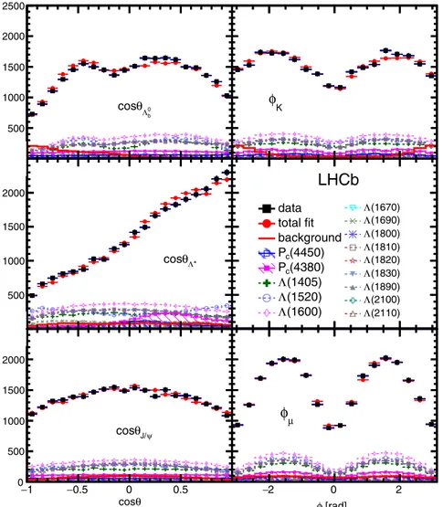
4449.8! 1.7 MeV and width 39 ! 5 MeV. These errors are statistical only; systematic uncertainties are discussed later. The mass resolution is approximately 2.5 MeV and does not affect the width determinations. The sFit approach gives comparable results. The angular distributions are reasonably well reproduced, as shown in Fig.7, and the comparison with the data in mKpintervals is also
satisfac-tory as can be seen in Fig.8. Interference effects between
θ cos 1 − −0.5 0 0.5 1 0 500 1000 1500 2000 2500 0 b Λ θ cos [rad] φ 2 − 0 2 0 K φ θ cos 1 − −0.5 0 0.5 1 0 500 1000 1500 2000 * Λ θ cos [rad] φ 2 − 0 2 0
LHCb
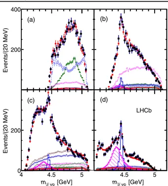
data total fit background (4450) c P (4380) c P (1405) Λ (1520) Λ (1600) Λ (1670) Λ (1690) Λ (1800) Λ (1810) Λ (1820) Λ (1830) Λ (1890) Λ (2100) Λ (2110) Λ θ cos 1 − −0.5 0 0.5 0 500 1000 1500 2000 ψ J/ θ cos [rad] φ 2 − 0 2 µ φFIG. 7 (color online). Various decay angular distributions for the fit with two Pþc states. The data are shown as (black) squares, while
the two Pþc states are particularly evident in Fig. 8(d),
where there is a large destructive contribution (not explic-itly shown in the figure) to the total rate. (A fit fraction comparison between cFit and sFit is given in the Supplemental Material [20].) The addition of further Pþc
states does not significantly improve the fit.
Adding a single 5=2þPþc state to the fit with only Λ%
states reduces−2 ln L by 14.72 using the extended model
and adding a second lower mass 3=2−Pþc state results in a
further reduction of 11.62. The combined reduction of
−2 ln L by the two states taken together is 18.72. Since
taking pffiffiffiffiffiffiffiffiffiffiffiffiffiffiffiΔ2 ln L overestimates significances, we perform simulations to obtain more accurate evaluations. We gen-erate pseudoexperiments using the null hypotheses having amplitude parameters determined by the fits to the data with no or one Pþc state. We fit each pseudoexperiment with the
null hypothesis and with Pþc states added to the model. The
−2 ln L distributions obtained from many pseudoexperi-ments are consistent with χ2distributions with the number
of degrees of freedom approximately equal to twice the number of extra parameters in the fit. Comparing these distributions with the Δ2 ln L values from the fits to the data, p values can be calculated. These studies show reduction of the significances relative to pffiffiffiffiffiffiffiffiffiffiffiffiffiffiffiΔ2 ln L by about 20%, giving overall significances of 9σ and 12σ,
for the lower and higher mass Pþc states, respectively. The
combined significance of two Pþc states is 15σ. Use of
the extended model to evaluate the significance includes the effect of systematic uncertainties due to the possible presence of additional Λ% states or higher L amplitudes.
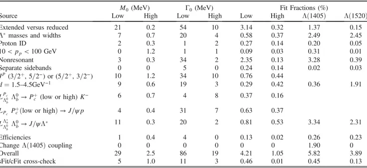
Systematic uncertainties are evaluated for the masses, widths, and fit fractions of the Pþc states, and for the fit
fractions of the two lightest and most significant Λ%states.
Additional sources of modeling uncertainty that we have not considered may affect the fit fractions of the heavier Λ%
states. The sources of systematic uncertainties are listed in TableII. They include differences between the results of the extended versus reduced model, varying the Λ% masses
and widths, uncertainties in the identification requirements for the proton and restricting its momentum, inclusion of a nonresonant amplitude in the fit, use of separate higher and lower Λ0
b mass sidebands, alternate JP fits, varying
the Blatt-Weisskopf barrier factor d between 1.5 and 4.5 GeV−1, changing the angular momentum L used in Eq.(5)by one or two units, and accounting for potential mismodeling of the efficiencies. For the Λð1405Þ fit fraction we also added an uncertainty for the Flatté couplings, determined by both halving and doubling their ratio, and taking the maximum deviation as the uncertainty. The stability of the results is cross-checked by compar-ing the data recorded in 2011 (2012), with the LHCb dipole magnet polarity in up (down) configurations, Λ0
bð ¯Λ0bÞ
decays, and Λ0
b produced with low (high) values of pT.
Extended model fits without including Pþc states were tried
with the addition of two high mass Λ%resonances of freely
varied mass and width, or four nonresonant components up to spin 3=2; these do not explain the data. The fitters were tested on simulated pseudoexperiments and no biases were found. In addition, selection requirements are varied, and the vetoes of ¯B0
sand ¯B0are removed and explicit models of
those backgrounds added to the fit; all give consistent results.
Further evidence for the resonant character of the higher mass, narrower Pþc state is obtained by viewing the
evolution of the complex amplitude in the Argand diagram
[12]. In the amplitude fits discussed above, the Pcð4450Þþ
is represented by a Breit-Wigner amplitude, where the magnitude and phase vary with mJ=ψp according to an
approximately circular trajectory in the (ReAPc, ImAPc)
plane, where APc is the mJ=ψp dependent part of the
Pcð4450Þþ amplitude. We perform an additional fit to
the data using the reduced Λ%model, in which we represent
the Pcð4450Þþ amplitude as the combination of
indepen-dent complex amplitudes at six equidistant points in the range !Γ0 ¼ 39 MeV around M0¼ 4449.8 MeV as
deter-mined in the default fit. Real and imaginary parts of the amplitude are interpolated in the mass interval between the fitted points. The resulting Argand diagram, shown in Fig. 9(a), is consistent with a rapid counterclockwise change of the Pcð4450Þþphase when its magnitude reaches
Events/(20 MeV) 0 200 400 (a) (b) [GeV] p ψ J/ m 4 4.5 5 Events/(20 MeV) 0 200 (c) [GeV] p ψ J/ m 4 4.5 5 (d) LHCb
FIG. 8 (color online). mJ=ψp in various intervals of mKp
for the fit with two Pþc states: (a) mKp< 1.55 GeV, (b)
1.55 < mKp< 1.70 GeV, (c) 1.70 < mKp< 2.00 GeV, and
(d) mKp> 2.00 GeV. The data are shown as (black) squares
with error bars, while the (red) circles show the results of the fit. The blue and purple histograms show the two Pþc states. See
the maximum, a behavior characteristic of a resonance. A similar study for the wider state is shown in Fig. 9(b); although the fit does show a large phase change, the amplitude values are sensitive to the details of the Λ%
model and so this latter study is not conclusive.
Different binding mechanisms of pentaquark states are possible. Tight binding was envisioned originally
[3,4,36]. A possible explanation is heavy-light diquarks
[37]. Examples of other mechanisms include a
diquark-diquark-antiquark model [38,39], a diquark-triquark model [40], and a coupled channel model [41]. Weakly bound “molecules” of a baryon plus a meson have been also discussed[42].
Models involving thresholds or “cusps” have been invoked to explain some exotic meson candidates via nonresonant scattering mechanisms [43–45]. There are certain obvious difficulties with the use of this approach to explain our results. The closest threshold to the high TABLE II. Summary of systematic uncertainties on Pþ
c masses, widths, and fit fractions, and Λ%fit fractions. A fit fraction is the ratio
of the phase space integrals of the matrix element squared for a single resonance and for the total amplitude. The terms “low” and “high” correspond to the lower and higher mass Pþc states. The sFit–cFit difference is listed as a cross-check and not included as an uncertainty.
M0(MeV) Γ0 (MeV) Fit Fractions (%)
Source Low High Low High Low High Λð1405Þ Λð1520Þ
Extended versus reduced 21 0.2 54 10 3.14 0.32 1.37 0.15
Λ% masses and widths 7 0.7 20 4 0.58 0.37 2.49 2.45
Proton ID 2 0.3 1 2 0.27 0.14 0.20 0.05 10 < pp< 100 GeV 0 1.2 1 1 0.09 0.03 0.31 0.01 Nonresonant 3 0.3 34 2 2.35 0.13 3.28 0.39 Separate sidebands 0 0 5 0 0.24 0.14 0.02 0.03 JP (3=2þ, 5=2−) or (5=2þ, 3=2−) 10 1.2 34 10 0.76 0.44 d ¼ 1.5–4.5GeV−1 9 0.6 19 3 0.29 0.42 0.36 1.91 LPc Λ0 b Λ 0 b→ Pþc (low or high) K− 6 0.7 4 8 0.37 0.16 LPc Pþcðlow or highÞ → J=ψp 4 0.4 31 7 0.63 0.37 LΛ%n Λ0 b Λ 0 b→ J=ψΛ% 11 0.3 20 2 0.81 0.53 3.34 2.31 Efficiencies 1 0.4 4 0 0.13 0.02 0.26 0.23 Change Λð1405Þ coupling 0 0 0 0 0 0 1.90 0 Overall 29 2.5 86 19 4.21 1.05 5.82 3.89 sFit/cFit cross-check 5 1.0 11 3 0.46 0.01 0.45 0.13 Re A -0.35 -0.3 -0.25 -0.2 -0.15 -0.1 -0.05 0 0.05 0.1 0.1 -0.35 -0.3 -0.25 -0.2 -0.15 -0.1 -0.05 0 0.05 0.1 0.15 LHCb (4450) c P (a) 5 -0.1 -0.05 0 0.05 0.1 0.15 0.2 0.25 0.3 0.35 (4380) c P (b) Pc Re APc Im A Pc
FIG. 9 (color online). Fitted values of the real and imaginary parts of the amplitudes for the baseline (3=2−, 5=2þ) fit for (a) the
Pcð4450Þþ state and (b) the Pcð4380Þþ state, each divided into six mJ=ψpbins of equal width between−Γ0 and þΓ0shown in the
Argand diagrams as connected points with error bars (mJ=ψpincreases counterclockwise). The solid (red) curves are the predictions from
the Breit-Wigner formula for the same mass ranges with M0(Γ0) of 4450 (39) MeV and 4380 (205) MeV, respectively, with the phases
and magnitudes at the resonance masses set to the average values between the two points around M0. The phase convention sets
B0;1
mass state is at 4457.1 ! 0.3 MeV resulting from a Λcð2595ÞþD¯0 combination, which is somewhat higher
than the peak mass value and would produce a structure with quantum numbers JP¼ 1=2þwhich are disfavored by
our data. There is no threshold close to the lower mass state. In conclusion, we have presented a full amplitude fit to the Λ0
b→ J=ψK−p decay. We observe significant Λ%
production recoiling against the J=ψ with the lowest mass contributions, the Λð1405Þ and Λð1520Þ states having fit fractions of ð15 ! 1 ! 6Þ% and ð19 ! 1 ! 4Þ%, respec-tively. The data cannot be satisfactorily described without including two Breit-Wigner shaped resonances in the J=ψp invariant mass distribution. The significances of the lower mass and higher mass states are 9 and 12 standard deviations, respectively. These structures cannot be accounted for by reflections from J=ψΛ% resonances or
other known sources. Interpreted as resonant states they must have minimal quark content of c¯cuud, and would therefore be called charmonium-pentaquark states. The lighter state Pcð4380Þþ has a mass of 4380!8!29 MeV
and a width of 205 ! 18 ! 86 MeV, while the heavier state Pcð4450Þþ has a mass of 4449.8 ! 1.7 ! 2.5 MeV and a
width of 39 ! 5 ! 19 MeV. A model-independent repre-sentation of the Pcð4450Þþ contribution in the fit shows a
phase change in amplitude consistent with that of a resonance. The parities of the two states are opposite with the preferred spins being 3=2 for one state and 5=2 for the other. The higher mass state has a fit fraction of ð4.1 ! 0.5 ! 1.1Þ%, and the lower mass state of ð8.4 ! 0.7 ! 4.2Þ%, of the total Λ0
b→ J=ψK−p sample.
We express our gratitude to our colleagues in the CERN accelerator departments for the excellent performance of the LHC. We thank the technical and administrative staff at the LHCb institutes. We acknowledge support from CERN and from the national agencies: CAPES, CNPq, FAPERJ, and FINEP (Brazil); NSFC (China); CNRS/IN2P3 (France); BMBF, DFG, HGF, and MPG (Germany); INFN (Italy); FOM and NWO (The Netherlands); MNiSW and NCN (Poland); MEN/IFA (Romania); MinES and FANO (Russia); MinECo (Spain); SNSF and SER (Switzerland); NASU (Ukraine); STFC (U.K.); and NSF (U.S.). The Tier1 computing centers are supported by IN2P3 (France), KIT and BMBF (Germany), INFN (Italy), NWO and SURF (The Netherlands), PIC (Spain), and GridPP (United Kingdom). We are indebted to the com-munities behind the multiple open source software pack-ages on which we depend. We are also thankful for the computing resources and the access to software research and development tools provided by Yandex LLC (Russia). Individual groups or members have received support from EPLANET, Marie Skłodowska-Curie Actions, and ERC (European Union); Conseil général de Haute-Savoie, Labex ENIGMASS, and OCEVU, Région Auvergne (France); RFBR (Russia); XuntaGal and GENCAT (Spain); and the
Royal Society and Royal Commission for the Exhibition of 1851 (United Kingdom).
[1] M. Gell-Mann, A schematic model of baryons and mesons, Phys. Lett. 8, 214 (1964).
[2] G. Zweig, Report No. CERN-TH-401.
[3] R. L. Jaffe, Multiquark hadrons. I. Phenomenology of Q2Q¯2
mesons,Phys. Rev. D 15, 267 (1977).
[4] D. Strottman, Multi-quark baryons and the MIT bag model, Phys. Rev. D 20, 748 (1979); H. Hogaasen and P. Sorba, The systematics of possibly narrow quark states with baryon number one, Nucl. Phys. B145, 119 (1978).
[5] H. J. Lipkin, New possibilities for exotic hadrons: Anticharmed strange baryons, Phys. Lett. B 195, 484 (1987).
[6] K. H. Hicks, On the conundrum of the pentaquark, Eur. Phys. J. H 37, 1 (2012).
[7] S. K. Choi et al. (Belle Collaboration), Observation of a Resonancelike Structure in the π!ψ0 Mass Distribution in
Exclusive B → Kπ!ψ0 Decays, Phys. Rev. Lett. 100, 142001 (2008).
[8] K. Chilikin et al. (Belle Collaboration), Experimental constraints on the spin and parity of the Zð4430Þþ, Phys. Rev. D 88, 074026 (2013).
[9] R. Aaij et al. (LHCb Collaboration), Observation of the Resonant Character of the Zð4430Þ−State,Phys. Rev. Lett. 112, 222002 (2014).
[10] X.-Q. Li and X. Liu, A possible global group structure for exotic states,Eur. Phys. J. C 74, 3198 (2014).
[11] R. Aaij et al. (LHCb Collaboration), Precision measurement of the ratio of the Λ0
bto ¯B0lifetimes,Phys. Lett. B 734, 122 (2014); Precision Measurement of the Λ0
bBaryon Lifetime, Phys. Rev. Lett. 111, 102003 (2013).
[12] K. A. Olive et al. (Particle Data Group), Review of particle physics,Chin. Phys. C 38, 090001 (2014).
[13] A. A. Alves Jr. et al. (LHCb Collaboration), The LHCb detector at the LHC, JINST 3, S08005 (2008).
[14] R. Aaij et al., Performance of the LHCb vertex locator, JINST 9, P09007 (2014).
[15] R. Arink et al., Performance of the LHCb outer tracker, JINST 9, P01002 (2014).
[16] M. Adinolfi et al., Performance of the LHCb RICH detector at the LHC, Eur. Phys. J. C 73, 2431 (2013).
[17] A. A. Alves Jr. et al., Performance of the LHCb muon system,JINST 8, P02022 (2013).
[18] R. Aaij et al. (LHCb Collaboration), First observation of B0
s → J=ψf0ð980Þ decays,Phys. Lett. B 698, 115 (2011).
[19] L. Breiman, J. H. Friedman, R. A. Olshen, and C. J. Stone, Classification and Regression Trees (Wadsworth International Group, Belmont, CA, 1984); A. Hoecker et al., TMVA: Toolkit for multivariate data analysis, Proc. Sci., ACAT (2007) 040 [arXiv:physics/0703039].
[20] See Supplemental Material at http://link.aps.org/ supplemental/10.1103/PhysRevLett.115.072001 for addi-tional information on the variables used in the BDTG, additional fit results, the fit fraction comparison between cFit and sFit, and details of the decay amplitude and fitting techniques.
[21] T. Sjöstrand, S. Mrenna, and P. Skands, PYTHIA 6.4 physics and manual, J. High Energy Phys. 05 (2006) 026; T. Sjöstrand, S. Mrenna, and P. Skands, A brief introduction to PYTHIA 8.1, Comput. Phys. Commun. 178, 852 (2008).
[22] I. Belyaev et al., Handling of the generation of primary events in Gauss, the LHCb simulation framework,J. Phys. Conf. Ser. 331, 032047 (2011).
[23] S. Agostinelli et al. (Geant4 Collaboration), Geant4: A simulation toolkit,Nucl. Instrum. Methods Phys. Res., Sect. A 506, 250 (2003); J. Allison et al. (Geant4 Collaboration), Geant4 developments and applications,IEEE Trans. Nucl. Sci. 53, 270 (2006).
[24] M. Clemencic, G. Corti, S. Easo, C. R. Jones, S. Miglioranzi, M. Pappagallo, and P. Robbe, The LHCb simulation appli-cation, Gauss: Design, evolution, and experience,J. Phys. Conf. Ser. 331, 032023 (2011).
[25] D. Martínez Santos and F. Dupertuis, Mass distributions marginalized over per-event errors,Nucl. Instrum. Methods Phys. Res., Sect. A 764, 150 (2014).
[26] W. D. Hulsbergen, Decay chain fitting with a Kalman filter, Nucl. Instrum. Methods Phys. Res., Sect. A 552, 566 (2005). [27] R. H. Dalitz, On the analysis of τ-meson data and the nature
of the τ meson,Philos. Mag. Ser. 5 44, 1068 (1953). [28] S. U. Chung, Report No. CERN-71-08; J. D. Richman,
Report No. CALT-68-1148; M. Jacob and G. C. Wick, On the general theory of collisions for particles with spin, Ann. Phys. (N.Y.) 7, 404 (1959).
[29] F. Von Hippel and C. Quigg, Centrifugal-barrier effects in resonance partial decay widths, shapes, and production amplitudes,Phys. Rev. D 5, 624 (1972).
[30] S. M. Flatté, Coupled-channel analysis of the πη and K ¯K systems near K ¯K threshold, Phys. Lett. 63B, 224 (1976).
[31] J. Soffer and N. A. Tornqvist, Origin of the Polarization for Inclusive Λ Production in pp Collisions,Phys. Rev. Lett. 68, 907 (1992).
[32] M. Pivk and F. R. Le Diberder, sPlot: A statistical tool to unfold data distributions, Nucl. Instrum. Methods Phys. Res., Sect. A 555, 356 (2005).
[33] F. James, Statistical Methods in Experimental Physics (World Scientific Publishing, Singapore, 2006).
[34] J. F. Donoghue, E. Golowich, W. A. Ponce, and B. R. Holstein, Analysis of ΔS ¼ 1 nonleptonic weak decays and theΔI ¼1
2rule,Phys. Rev. D 21, 186 (1980).
[35] R. Aaij et al. (LHCb Collaboration), Observation of Over-lapping Spin-1 and Spin-3 ¯D0K− Resonances at Mass
2.86 GeV=c2,Phys. Rev. Lett. 113, 162001 (2014); Dalitz
plot analysis of B0
s→ ¯D0K−πþ decays,Phys. Rev. D 90, 072003 (2014).
[36] G. C. Rossi and G. Veneziano, A possible description of baryon dynamics in dual and gauge theories, Nucl. Phys. B123, 507 (1977).
[37] L. Maiani, F. Piccinini, A. D. Polosa, and V. Riquer, Diquark-antidiquarks with hidden or open charm and the nature of Xð3872Þ,Phys. Rev. D 71, 014028 (2005). [38] R. Jaffe and F. Wilczek, Diquarks and Exotic Spectroscopy,
Phys. Rev. Lett. 91, 232003 (2003).
[39] A. Chandra, A. Bhattacharya, and B. Chakrabarti, Heavy pentaquarks and doubly heavy baryons in quasiparticle approach, Mod. Phys. Lett. A 27, 1250006 (2012).
[40] M. Karliner and H. J. Lipkin, A diquark-triquark model for the KN pentaquark,Phys. Lett. B 575, 249 (2003). [41] J.-J. Wu, R. Molina, E. Oset, and B. S. Zou, Prediction of
Narrow N%and Λ%Resonances with Hidden Charm Above
4 GeV,Phys. Rev. Lett. 105, 232001 (2010).
[42] M. B. Voloshin and L. B. Okun, Hadron molecules and charmonium atom, JETP Lett. 23, 333 (1976); A. De Rujula, H. Georgi, and S. L. Glashow, Molecular Charmo-nium: A New Spectroscopy?, Phys. Rev. Lett. 38, 317 (1977); N. A. Törnqvist, Possible Large Deuteronlike Meson-Meson States Bound by Pions, Phys. Rev. Lett. 67, 556 (1991); N. A. Törnqvist, From the deuteron to deusons, an analysis of deuteron-like meson-meson bound states,Z. Phys. C 61, 525 (1994); Z.-C. Yang, Z.-F. Sun, J. He, X. Liu, and S.-L. Zhu, The possible hidden-charm molecular baryons composed of anti-charmed meson and charmed baryon,Chin. Phys. C 36, 6 (2012); W. L. Wang, F. Huang, Z. Y. Zhang, and B. S. Zou,ΣcD and Λ¯ cD states¯
in a chiral quark model,Phys. Rev. C 84, 015203 (2011); M. Karliner and J. L. Rosner, New exotic meson and baryon resonances from doubly-heavy hadronic molecules,arXiv: 1506.06386.
[43] E. S. Swanson, Cusps and exotic charmonia, arXiv: 1504.07952.
[44] E. S. Swanson, Zband Zcexotic states as coupled channel
cusps,Phys. Rev. D 91, 034009 (2015).
[45] D. V. Bugg, An explanation of Belle states Zbð10610Þ and
Zbð10650Þ,Europhys. Lett. 96, 11002 (2011).
R. Aaij,38 B. Adeva,37 M. Adinolfi,46 A. Affolder,52 Z. Ajaltouni,5S. Akar,6J. Albrecht,9F. Alessio,38 M. Alexander,51 S. Ali,41G. Alkhazov,30P. Alvarez Cartelle,53A. A. Alves Jr.,57S. Amato,2S. Amerio,22Y. Amhis,7L. An,3L. Anderlini,17 J. Anderson,40G. Andreassi,39M. Andreotti,16,fJ. E. Andrews,58R. B. Appleby,54O. Aquines Gutierrez,10 F. Archilli,38 P. d’Argent,11A. Artamonov,35M. Artuso,59E. Aslanides,6G. Auriemma,25,mM. Baalouch,5S. Bachmann,11J. J. Back,48
A. Badalov,36 C. Baesso,60 W. Baldini,16,38R. J. Barlow,54 C. Barschel,38 S. Barsuk,7 W. Barter,38 V. Batozskaya,28
V. Battista,39 A. Bay,39 L. Beaucourt,4 J. Beddow,51 F. Bedeschi,23 I. Bediaga,1 L. J. Bel,41 V. Bellee,39 N. Belloli,20 I. Belyaev,31 E. Ben-Haim,8 G. Bencivenni,18 S. Benson,38 J. Benton,46 A. Berezhnoy,32 R. Bernet,40 A. Bertolin,22 M.-O. Bettler,38M. van Beuzekom,41A. Bien,11S. Bifani,45P. Billoir,8T. Bird,54A. Birnkraut,9A. Bizzeti,17,hT. Blake,48
T. J. V. Bowcock,52 E. Bowen,40 C. Bozzi,16 S. Braun,11 M. Britsch,10 T. Britton,59 J. Brodzicka,54 N. H. Brook,46 A. Bursche,40J. Buytaert,38 S. Cadeddu,15R. Calabrese,16,f M. Calvi,20,j M. Calvo Gomez,36,oP. Campana,18 D. Campora Perez,38L. Capriotti,54A. Carbone,14,dG. Carboni,24,kR. Cardinale,19,iA. Cardini,15P. Carniti,20L. Carson,50
K. Carvalho Akiba,2,38G. Casse,52L. Cassina,20,j L. Castillo Garcia,38M. Cattaneo,38Ch. Cauet,9G. Cavallero,19 R. Cenci,23,sM. Charles,8Ph. Charpentier,38M. Chefdeville,4S. Chen,54S.-F. Cheung,55N. Chiapolini,40M. Chrzaszcz,40
X. Cid Vidal,38 G. Ciezarek,41 P. E. L. Clarke,50 M. Clemencic,38 H. V. Cliff,47 J. Closier,38V. Coco,38J. Cogan,6 E. Cogneras,5V. Cogoni,15,eL. Cojocariu,29G. Collazuol,22P. Collins,38A. Comerma-Montells,11A. Contu,15,38A. Cook,46
M. Coombes,46 S. Coquereau,8 G. Corti,38M. Corvo,16,fB. Couturier,38 G. A. Cowan,50 D. C. Craik,48A. Crocombe,48
M. Cruz Torres,60S. Cunliffe,53R. Currie,53C. D’Ambrosio,38E. Dall’Occo,41J. Dalseno,46P. N. Y. David,41A. Davis,57
K. De Bruyn,41S. De Capua,54M. De Cian,11J. M. De Miranda,1L. De Paula,2P. De Simone,18C.-T. Dean,51D. Decamp,4 M. Deckenhoff,9 L. Del Buono,8N. Déléage,4M. Demmer,9 D. Derkach,55 O. Deschamps,5F. Dettori,38 B. Dey,21 A. Di Canto,38 F. Di Ruscio,24H. Dijkstra,38 S. Donleavy,52 F. Dordei,11 M. Dorigo,39 A. Dosil Suárez,37 D. Dossett,48
A. Dovbnya,43 K. Dreimanis,52 L. Dufour,41G. Dujany,54 F. Dupertuis,39 P. Durante,38 R. Dzhelyadin,35 A. Dziurda,26 A. Dzyuba,30 S. Easo,49,38U. Egede,53 V. Egorychev,31 S. Eidelman,34 S. Eisenhardt,50 U. Eitschberger,9R. Ekelhof,9 L. Eklund,51I. El Rifai,5 Ch. Elsasser,40 S. Ely,59S. Esen,11 H. M. Evans,47 T. Evans,55A. Falabella,14 C. Färber,38 N. Farley,45S. Farry,52R. Fay,52D. Ferguson,50V. Fernandez Albor,37F. Ferrari,14F. Ferreira Rodrigues,1M. Ferro-Luzzi,38 S. Filippov,33M. Fiore,16,38,fM. Fiorini,16,fM. Firlej,27C. Fitzpatrick,39T. Fiutowski,27K. Fohl,38P. Fol,53M. Fontana,15 F. Fontanelli,19,iR. Forty,38O. Francisco,2M. Frank,38C. Frei,38M. Frosini,17J. Fu,21E. Furfaro,24,kA. Gallas Torreira,37 D. Galli,14,dS. Gallorini,22,38S. Gambetta,50M. Gandelman,2P. Gandini,55Y. Gao,3J. García Pardiñas,37J. Garra Tico,47
L. Garrido,36D. Gascon,36C. Gaspar,38R. Gauld,55L. Gavardi,9G. Gazzoni,5A. Geraci,21,uD. Gerick,11E. Gersabeck,11
M. Gersabeck,54 T. Gershon,48 Ph. Ghez,4 A. Gianelle,22S. Gianì,39 V. Gibson,47 O. G. Girard,39 L. Giubega,29
V. V. Gligorov,38 C. Göbel,60 D. Golubkov,31A. Golutvin,53,31,38 A. Gomes,1,a C. Gotti,20,j M. Grabalosa Gándara,5 R. Graciani Diaz,36L. A. Granado Cardoso,38E. Graugés,36 E. Graverini,40 G. Graziani,17 A. Grecu,29E. Greening,55 S. Gregson,47P. Griffith,45L. Grillo,11O. Grünberg,63B. Gui,59E. Gushchin,33Yu. Guz,35,38T. Gys,38T. Hadavizadeh,55 C. Hadjivasiliou,59G. Haefeli,39C. Haen,38S. C. Haines,47S. Hall,53B. Hamilton,58X. Han,11S. Hansmann-Menzemer,11
N. Harnew,55 S. T. Harnew,46 J. Harrison,54 J. He,38T. Head,39V. Heijne,41K. Hennessy,52 P. Henrard,5L. Henry,8 J. A. Hernando Morata,37E. van Herwijnen,38M. Heß,63 A. Hicheur,2 D. Hill,55 M. Hoballah,5C. Hombach,54 W. Hulsbergen,41T. Humair,53N. Hussain,55D. Hutchcroft,52D. Hynds,51M. Idzik,27P. Ilten,56R. Jacobsson,38A. Jaeger,11 J. Jalocha,55E. Jans,41A. Jawahery,58F. Jing,3M. John,55 D. Johnson,38C. R. Jones,47C. Joram,38B. Jost,38N. Jurik,59 S. Kandybei,43 W. Kanso,6M. Karacson,38 T. M. Karbach,38,† S. Karodia,51 M. Kecke,11M. Kelsey,59I. R. Kenyon,45
M. Kenzie,38T. Ketel,42 B. Khanji,20,38,j C. Khurewathanakul,39S. Klaver,54 K. Klimaszewski,28 O. Kochebina,7
M. Kolpin,11I. Komarov,39R. F. Koopman,42P. Koppenburg,41,38M. Kozeiha,5L. Kravchuk,33K. Kreplin,11M. Kreps,48
G. Krocker,11 P. Krokovny,34 F. Kruse,9W. Krzemien,28W. Kucewicz,26,nM. Kucharczyk,26V. Kudryavtsev,34
A. K. Kuonen,39 K. Kurek,28T. Kvaratskheliya,31 D. Lacarrere,38G. Lafferty,54A. Lai,15D. Lambert,50G. Lanfranchi,18 C. Langenbruch,48 B. Langhans,38 T. Latham,48C. Lazzeroni,45R. Le Gac,6 J. van Leerdam,41 J.-P. Lees,4R. Lefèvre,5
A. Leflat,32,38 J. Lefrançois,7 O. Leroy,6T. Lesiak,26B. Leverington,11 Y. Li,7 T. Likhomanenko,65,64 M. Liles,52 R. Lindner,38 C. Linn,38F. Lionetto,40 B. Liu,15 X. Liu,3D. Loh,48I. Longstaff,51 J. H. Lopes,2 D. Lucchesi,22,q M. Lucio Martinez,37 H. Luo,50 A. Lupato,22 E. Luppi,16,f O. Lupton,55N. Lusardi,21A. Lusiani,23F. Machefert,7 F. Maciuc,29O. Maev,30K. Maguire,54S. Malde,55A. Malinin,64G. Manca,7G. Mancinelli,6P. Manning,59A. Mapelli,38 J. Maratas,5J. F. Marchand,4U. Marconi,14C. Marin Benito,36P. Marino,23,38,sJ. Marks,11G. Martellotti,25 M. Martin,6 M. Martinelli,39D. Martinez Santos,37F. Martinez Vidal,66D. Martins Tostes,2A. Massafferri,1R. Matev,38A. Mathad,48
Z. Mathe,38 C. Matteuzzi,20 A. Mauri,40 B. Maurin,39 A. Mazurov,45M. McCann,53 J. McCarthy,45 A. McNab,54
R. McNulty,12 B. Meadows,57 F. Meier,9M. Meissner,11D. Melnychuk,28M. Merk,41D. A. Milanes,62 M.-N. Minard,4
D. S. Mitzel,11 J. Molina Rodriguez,60 I. A. Monroy,62 S. Monteil,5 M. Morandin,22 P. Morawski,27 A. Mordà,6
M. J. Morello,23,sJ. Moron,27A. B. Morris,50R. Mountain,59F. Muheim,50J. Müller,9K. Müller,40V. Müller,9M. Mussini,14
B. Muster,39P. Naik,46 T. Nakada,39R. Nandakumar,49A. Nandi,55 I. Nasteva,2M. Needham,50N. Neri,21S. Neubert,11 N. Neufeld,38 M. Neuner,11 A. D. Nguyen,39 T. D. Nguyen,39 C. Nguyen-Mau,39,p V. Niess,5 R. Niet,9N. Nikitin,32 T. Nikodem,11 D. Ninci,23A. Novoselov,35 D. P. O’Hanlon,48 A. Oblakowska-Mucha,27 V. Obraztsov,35 S. Ogilvy,51 O. Okhrimenko,44 R. Oldeman,15,e C. J. G. Onderwater,67 B. Osorio Rodrigues,1 J. M. Otalora Goicochea,2 A. Otto,38
P. Owen,53 A. Oyanguren,66A. Palano,13,cF. Palombo,21,tM. Palutan,18 J. Panman,38A. Papanestis,49 M. Pappagallo,51 L. L. Pappalardo,16,fC. Pappenheimer,57C. Parkes,54G. Passaleva,17 G. D. Patel,52M. Patel,53 C. Patrignani,19,i A. Pearce,54,49A. Pellegrino,41G. Penso,25,l M. Pepe Altarelli,38S. Perazzini,14,dP. Perret,5L. Pescatore,45K. Petridis,46
A. Petrolini,19,i M. Petruzzo,21E. Picatoste Olloqui,36B. Pietrzyk,4 T. Pilař,48 D. Pinci,25A. Pistone,19 A. Piucci,11
S. Playfer,50M. Plo Casasus,37 T. Poikela,38F. Polci,8A. Poluektov,48,34I. Polyakov,31E. Polycarpo,2 A. Popov,35 D. Popov,10,38B. Popovici,29 C. Potterat,2 E. Price,46J. D. Price,52 J. Prisciandaro,39 A. Pritchard,52 C. Prouve,46 V. Pugatch,44A. Puig Navarro,39G. Punzi,23,rW. Qian,4R. Quagliani,7,46B. Rachwal,26J. H. Rademacker,46M. Rama,23
M. S. Rangel,2 I. Raniuk,43N. Rauschmayr,38G. Raven,42 F. Redi,53S. Reichert,54 M. M. Reid,48 A. C. dos Reis,1
S. Ricciardi,49S. Richards,46M. Rihl,38K. Rinnert,52V. Rives Molina,36P. Robbe,7,38A. B. Rodrigues,1E. Rodrigues,54
J. A. Rodriguez Lopez,62 P. Rodriguez Perez,54 S. Roiser,38V. Romanovsky,35A. Romero Vidal,37 J. W. Ronayne,12 M. Rotondo,22 J. Rouvinet,39T. Ruf,38 P. Ruiz Valls,66 J. J. Saborido Silva,37 N. Sagidova,30 P. Sail,51 B. Saitta,15,e V. Salustino Guimaraes,2C. Sanchez Mayordomo,66B. Sanmartin Sedes,37 R. Santacesaria,25 C. Santamarina Rios,37 M. Santimaria,18E. Santovetti,24,kA. Sarti,18,lC. Satriano,25,mA. Satta,24D. M. Saunders,46D. Savrina,31,32M. Schiller,38
H. Schindler,38M. Schlupp,9M. Schmelling,10T. Schmelzer,9B. Schmidt,38O. Schneider,39A. Schopper,38M. Schubiger,39 M.-H. Schune,7R. Schwemmer,38 B. Sciascia,18A. Sciubba,25,lA. Semennikov,31 N. Serra,40J. Serrano,6 L. Sestini,22 P. Seyfert,20 M. Shapkin,35 I. Shapoval,16,43,fY. Shcheglov,30 T. Shears,52L. Shekhtman,34 V. Shevchenko,64A. Shires,9 B. G. Siddi,16R. Silva Coutinho,48G. Simi,22M. Sirendi,47N. Skidmore,46I. Skillicorn,51T. Skwarnicki,59E. Smith,55,49 E. Smith,53I. T. Smith,50J. Smith,47M. Smith,54H. Snoek,41M. D. Sokoloff,57,38F. J. P. Soler,51F. Soomro,39D. Souza,46
B. Souza De Paula,2B. Spaan,9P. Spradlin,51 S. Sridharan,38 F. Stagni,38 M. Stahl,11 S. Stahl,38 S. Stefkova,53 O. Steinkamp,40O. Stenyakin,35S. Stevenson,55 S. Stoica,29 S. Stone,59B. Storaci,40 S. Stracka,23,sM. Straticiuc,29 U. Straumann,40L. Sun,57W. Sutcliffe,53K. Swientek,27S. Swientek,9V. Syropoulos,42M. Szczekowski,28P. Szczypka,39,38 T. Szumlak,27 S. T’Jampens,4A. Tayduganov,6T. Tekampe,9M. Teklishyn,7G. Tellarini,16,f F. Teubert,38 C. Thomas,55
E. Thomas,38 J. van Tilburg,41 V. Tisserand,4 M. Tobin,39 J. Todd,57 S. Tolk,42L. Tomassetti,16,fD. Tonelli,38
S. Topp-Joergensen,55 N. Torr,55 E. Tournefier,4 S. Tourneur,39K. Trabelsi,39 M. T. Tran,39M. Tresch,40 A. Trisovic,38 A. Tsaregorodtsev,6P. Tsopelas,41N. Tuning,41,38A. Ukleja,28A. Ustyuzhanin,65,64U. Uwer,11C. Vacca,15,eV. Vagnoni,14 G. Valenti,14 A. Vallier,7R. Vazquez Gomez,18P. Vazquez Regueiro,37C. Vázquez Sierra,37S. Vecchi,16 J. J. Velthuis,46
M. Veltri,17,gG. Veneziano,39 M. Vesterinen,11B. Viaud,7D. Vieira,2 M. Vieites Diaz,37 X. Vilasis-Cardona,36,o
A. Vollhardt,40D. Volyanskyy,10 D. Voong,46 A. Vorobyev,30V. Vorobyev,34 C. Voß,63 J. A. de Vries,41 R. Waldi,63 C. Wallace,48 R. Wallace,12 J. Walsh,23 S. Wandernoth,11 J. Wang,59 D. R. Ward,47 N. K. Watson,45 D. Websdale,53 A. Weiden,40 M. Whitehead,48G. Wilkinson,55,38 M. Wilkinson,59 M. Williams,38 M. P. Williams,45 M. Williams,56 T. Williams,45 F. F. Wilson,49 J. Wimberley,58 J. Wishahi,9W. Wislicki,28 M. Witek,26G. Wormser,7S. A. Wotton,47 S. Wright,47K. Wyllie,38Y. Xie,61Z. Xu,39Z. Yang,3J. Yu,61X. Yuan,34O. Yushchenko,35M. Zangoli,14M. Zavertyaev,10,b
L. Zhang,3 Y. Zhang,3A. Zhelezov,11 A. Zhokhov,31 L. Zhong3 and S. Zucchelli14 (LHCb Collaboration)
1Centro Brasileiro de Pesquisas Físicas (CBPF), Rio de Janeiro, Brazil 2Universidade Federal do Rio de Janeiro (UFRJ), Rio de Janeiro, Brazil
3Center for High Energy Physics, Tsinghua University, Beijing, China 4LAPP, Université Savoie Mont-Blanc, CNRS/IN2P3, Annecy-Le-Vieux, France 5Clermont Université, Université Blaise Pascal, CNRS/IN2P3, LPC, Clermont-Ferrand, France
6CPPM, Aix-Marseille Université, CNRS/IN2P3, Marseille, France 7LAL, Université Paris-Sud, CNRS/IN2P3, Orsay, France
8LPNHE, Université Pierre et Marie Curie, Université Paris Diderot, CNRS/IN2P3, Paris, France 9Fakultät Physik, Technische Universität Dortmund, Dortmund, Germany
10Max-Planck-Institut für Kernphysik (MPIK), Heidelberg, Germany
11Physikalisches Institut, Ruprecht-Karls-Universität Heidelberg, Heidelberg, Germany 12School of Physics, University College Dublin, Dublin, Ireland
13Sezione INFN di Bari, Bari, Italy 14Sezione INFN di Bologna, Bologna, Italy 15Sezione INFN di Cagliari, Cagliari, Italy 16Sezione INFN di Ferrara, Ferrara, Italy
17Sezione INFN di Firenze, Firenze, Italy
18Laboratori Nazionali dell’INFN di Frascati, Frascati, Italy 19Sezione INFN di Genova, Genova, Italy
20Sezione INFN di Milano Bicocca, Milano, Italy 21Sezione INFN di Milano, Milano, Italy 22Sezione INFN di Padova, Padova, Italy
23Sezione INFN di Pisa, Pisa, Italy 24Sezione INFN di Roma Tor Vergata, Roma, Italy 25Sezione INFN di Roma La Sapienza, Roma, Italy
26Henryk Niewodniczanski Institute of Nuclear Physics Polish Academy of Sciences, Kraków, Poland 27AGH - University of Science and Technology, Faculty of Physics and Applied Computer Science, Kraków, Poland
28National Center for Nuclear Research (NCBJ), Warsaw, Poland
29Horia Hulubei National Institute of Physics and Nuclear Engineering, Bucharest-Magurele, Romania 30Petersburg Nuclear Physics Institute (PNPI), Gatchina, Russia
31Institute of Theoretical and Experimental Physics (ITEP), Moscow, Russia 32Institute of Nuclear Physics, Moscow State University (SINP MSU), Moscow, Russia 33Institute for Nuclear Research of the Russian Academy of Sciences (INR RAN), Moscow, Russia 34Budker Institute of Nuclear Physics (SB RAS) and Novosibirsk State University, Novosibirsk, Russia
35Institute for High Energy Physics (IHEP), Protvino, Russia 36Universitat de Barcelona, Barcelona, Spain
37Universidad de Santiago de Compostela, Santiago de Compostela, Spain 38European Organization for Nuclear Research (CERN), Geneva, Switzerland
39Ecole Polytechnique Fédérale de Lausanne (EPFL), Lausanne, Switzerland 40Physik-Institut, Universität Zürich, Zürich, Switzerland
41Nikhef National Institute for Subatomic Physics, Amsterdam, The Netherlands
42Nikhef National Institute for Subatomic Physics and VU University Amsterdam, Amsterdam, The Netherlands 43NSC Kharkiv Institute of Physics and Technology (NSC KIPT), Kharkiv, Ukraine
44Institute for Nuclear Research of the National Academy of Sciences (KINR), Kyiv, Ukraine 45University of Birmingham, Birmingham, United Kingdom
46H.H. Wills Physics Laboratory, University of Bristol, Bristol, United Kingdom 47Cavendish Laboratory, University of Cambridge, Cambridge, United Kingdom 48Department of Physics, University of Warwick, Coventry, United Kingdom
49STFC Rutherford Appleton Laboratory, Didcot, United Kingdom
50School of Physics and Astronomy, University of Edinburgh, Edinburgh, United Kingdom 51School of Physics and Astronomy, University of Glasgow, Glasgow, United Kingdom
52Oliver Lodge Laboratory, University of Liverpool, Liverpool, United Kingdom 53Imperial College London, London, United Kingdom
54School of Physics and Astronomy, University of Manchester, Manchester, United Kingdom 55Department of Physics, University of Oxford, Oxford, United Kingdom
56Massachusetts Institute of Technology, Cambridge, Massachusetts, USA 57University of Cincinnati, Cincinnati, Ohio, USA
58University of Maryland, College Park, Maryland, USA 59Syracuse University, Syracuse, New York, USA
60Pontifícia Universidade Católica do Rio de Janeiro (PUC-Rio), Rio de Janeiro,
Brazil (associated with Universidade Federal do Rio de Janeiro (UFRJ), Rio de Janeiro, Brazil)
61Institute of Particle Physics, Central China Normal University, Wuhan, Hubei,
China (associated with Center for High Energy Physics, Tsinghua University, Beijing, China)
62Departamento de Fisica, Universidad Nacional de Colombia, Bogota, Colombia
(associated with LPNHE, Université Pierre et Marie Curie, Université Paris Diderot, CNRS/IN2P3, Paris, France)
63Institut für Physik, Universität Rostock, Rostock, Germany (associated with Physikalisches Institut,
Ruprecht-Karls-Universität Heidelberg, Heidelberg, Germany)
64National Research Centre Kurchatov Institute, Moscow, Russia (associated with Institute of Theoretical
and Experimental Physics (ITEP), Moscow, Russia)
65Yandex School of Data Analysis, Moscow, Russia (associated with Institute of Theoretical and Experimental Physics (ITEP),
Moscow, Russia)
66Instituto de Fisica Corpuscular (IFIC), Universitat de Valencia-CSIC, Valencia, Spain
(associated with Universitat de Barcelona, Barcelona, Spain)
67Van Swinderen Institute, University of Groningen, Groningen, The Netherlands
†Deceased.
aAlso at Universidade Federal do Triângulo Mineiro (UFTM), Uberaba-MG, Brazil.
bAlso at P. N. Lebedev Physical Institute, Russian Academy of Science (LPI RAS), Moscow, Russia. cAlso at Università di Bari, Bari, Italy.
dAlso at Università di Bologna, Bologna, Italy. eAlso at Università di Cagliari, Cagliari, Italy. fAlso at Università di Ferrara, Ferrara, Italy. gAlso at Università di Urbino, Urbino, Italy.
hAlso at Università di Modena e Reggio Emilia, Modena, Italy. iAlso at Università di Genova, Genova, Italy.
jAlso at Università di Milano Bicocca, Milano, Italy. kAlso at Università di Roma Tor Vergata, Roma, Italy.
lAlso at Università di Roma La Sapienza, Roma, Italy. mAlso at Università della Basilicata, Potenza, Italy.
nAlso at AGH - University of Science and Technology, Faculty of Computer Science, Electronics and Telecommunications, Kraków, Poland.
oAlso at LIFAELS, La Salle, Universitat Ramon Llull, Barcelona, Spain. pAlso at Hanoi University of Science, Hanoi, Vietnam.
qAlso at Università di Padova, Padova, Italy. rAlso at Università di Pisa, Pisa, Italy. sAlso at Scuola Normale Superiore, Pisa, Italy.
tAlso at Università degli Studi di Milano, Milano, Italy. uAlso at Politecnico di Milano, Milano, Italy.
![TABLE I. The Λ % resonances used in the different fits. Parameters are taken from the PDG [12]](https://thumb-eu.123doks.com/thumbv2/123dokorg/4938003.51982/6.892.128.762.788.1038/table-resonances-used-different-fits-parameters-taken-pdg.webp)