Riassunto
L’argomento affrontato in questa tesi riguarda lo sviluppo di un modello a pa-rametri concentrati in grado di simulare il comportamento vibratorio di pompe a palette a cilindrata variabile. Si tratta di un modello piano a tre gradi di libert`a, deputato allo studio della dinamica delle parti in rotazione. Tale mo-dello considera l’azione delle forze di pressione variabili sul rotore, le reazioni dei cuscinetti idrodinamici, l’attrito dovuto alle azioni viscose ed alle forze di contatto, le propriet`a del rotore in termini di rigidezza e smorzamento, le va-riazioni della geometria della pompa in funzione delle condizioni di esercizio ed infine, tutte le azioni d’inerzia. In particolare, il calcolo delle forze e delle coppie di pressione `e svolto grazie alla valutazione preliminare del campo di pressione mediante un modello basato su un approccio euleriano che considera 26 volumi di controllo.
Il modello in questione pu`o quindi determinare il campo di pressione agente all’interno della pompa e calcolare le accelerazioni a cui `e sottoposto il rotore, le forze di reazione dei cuscinetti fluido-dinamici e la coppia motrice assorbita dalla pompa in condizioni operative.
Dopo la descrizione del modello dal punto di vista teorico, vengono presentati la campagna sperimentale ed il metodo di validazione. A tal pro si `e sviluppata un’originale metodologia, che consiste nel comparare le accelerazioni del corpo pompa calcolate servendosi del modello con le medesime accelerazioni misurate in condizioni di esercizio.
Infine alcuni significativi risultati vengono riportati quale esempio di appli-cazione.
Il principale contributo originale di questa tesi consiste nello sviluppo di un mo-dello dinamico non lineare di pompe a palette a cilindrata variabile che include simultaneamente i pi`u rilevanti fenomeni dinamici presenti nel funzionamento della pompa e la valutazione delle loro interazioni. Questa peculiarit`a pu`o essere importante al fine di investigare l’influenza di modifiche progettuali sul compor-tamento del sistema meccanico in questione e, in questo senso, il modello svilup-pato pu`o essere considerato un valido strumento di prototipazione, in grado di identificare l’origine di effetti dinamici indesiderati.
Abstract
This PhD thesis presents a lumped parameter model able to simulate the vi-brational behavior of a wide range of variable displacement vane pumps. The vibration analysis of the rotating parts is carried out through a planar model with three degrees of freedom. It takes into account the variability of the pres-sure loads acting on the rotor shaft, the hydrodynamic journal bearing reactions, the friction due to viscous actions and contact forces, the rotor shaft stiffness and damping, the variation of the pump geometry with respect to working con-dition and all the inertia actions. In particular, the computation of pressure forces and torques is allowed by the preliminary evaluation of the variable pres-sure field acting inside the pump, obtained through a model based on an Euler’s approach with 26 control volumes.
Thus, the present model makes it possible to define the pressure field acting inside the pump, and calculate the rotor shaft accelerations, as well as the journal bearing reaction forces and the motor drive torque absorbed by the pump in working condition.
The test campaign and the validation method are then described: an original assessment technique based on the comparison of pump casing accelerations is proposed.
Finally, some important simulation results are reported as an example of appli-cation.
The main original contribution of this work concerns the development of a non-linear model of variable displacement vane pumps including all the important dynamic effects in the same model, with the aim at taking into account their iterations. This can be important in order to foresee the influence of work-ing conditions and design modifications on the pump vibrational behavior. In this sense the developed lumped parameter model could be a very useful tool in prototype design, in order to identify the origin of unwanted dynamic effects.
Preface
Nowadays, increasing attention is addressed to vibro-acoustic problems in me-chanical systems to improve their performances in terms of precision, reliability and comfort. In this frame the research activity I carried out during my PhD has dealt with the development of methodologies and applicative tools integrat-ing vibro-acoustic modelintegrat-ing and experimental analysis with the aim to optimize the vibro-acoustic behavior of mechanical systems and to understand the com-plex phenomena related to their operational conditions. In more detail, my activity focused on the study of advanced modeling, simulation and experimen-tal assessment techniques for the characterization of complex machinery and physical systems. The two main topics I studied in the last three years are the nearfield structure-borne sound holography applied to shell shape elements and the lumped parameter modeling of variable displacement vane pumps. This last topic will be widely discussed in the present work.
When dealing with complex mechanical systems, such as variable displacement vane pumps, an accurate prediction of the system dynamical behavior is capi-tally important in a proper vibro-acoustical optimization. The first target is the simulation of the pressure field acting inside the pump. As a matter of fact the pressure fields is the main actor in determining the time variable loads acting on the pump casing. In this sight a zero-dymensional model, based on an Eu-ler’s approach has been developed allowing to compute the pressure evolution by solving a system of flow rate continuity equations. The results have been validated by comparison with experimental pressure evolutions. Furthermore, the forces exciting the rotor shaft have been calculated and used as input data for a kineto-elastodynamic model that analyzes the equilibrium between the re-sulting pressure forces, the journal bearings reactions and the inertial actions. In this way the variable forces exciting the pump casing in working condition are fully characterized.
Another important activity deals with the frequency response function of the pump casing. To do this, an original procedure has been studied to better simulate the pump behavior in working conditions.
Finally the model outputs in term of time varying forces and the experimental frequency response functions can be used to estimate the pump casing acceler-ations that are the main noise cause. Such a global analysis approach can be rarely found in the literature and involves a large number of modeling techniques at the same time.
pumps using different approaches”. By Meneghetti, U., Maggiore, A., Parenti Castelli, V., in Quarta Giornata di studio in onore di Ettore Funaioli, 16th July 2010, Ed. Asterisco, Bologna (acts in press).
The activity about nearfield structure-borne sound holography have been car-ried out during a period of six months I spent to the Department of Fluid Me-chanics and Engineering Acoustics of the Technische Universit¨at Berlin, under the supervision of Prof. B. A. T. Petersson. This project have been devel-oped in the frame of the EDSVS program (European Doctorate in Sound and Vibration Studies) with the aim at defining a new technique suitable to re-construct the velocity and force fields acting on the surface of a shell shape element with multiple excitation points (further information can be found at www.isvr.soton.ac.uk/edsvs/pro08 Marco Cavallari.htm). This novel approach allows to calculate the excitation forces starting from vibrational velocity mea-surements of the same structure in the near field. The structure has been modeled in MATLAB environment and the results have been experimentally assessed after having characterized the source-receiver coupling thanks to a test bench suitably designed. The promising results of this activity have been related in this publication:
Cavallari, M., Bonhoff, H. A., and Petersson B. A. T., 2009, ”Nearfield structure-borne sound holography”. In NOVEM 2009, 5−8 April 2009, Oxford.
Moreover, I worked in the diagnostics of mechanical systems by means of ad-vanced signal processing techniques. In this frame I developed the cyclosta-tionary modelling and other advanced techniques for the diagnosis of assembly faults in internal combustion engine cold tests; I studied polyurethane heavy-duty wheels for industrial applications to detect contamination faults and finally I worked on signal precessing techniques applied to fault detection in helical gearboxes.
Delvecchio, S., D’Elia, G., Cavallari, M., and Dalpiaz, G., 2008, ”Use of the cyclostationary modelling for the diagnosis of assembly faults in i.c. engine cold tests”. In Proceedings of ISMA2008, 15−17 September 2008, Leuven, Belgium.
Cavallari. M., D’Elia, G., Delvecchio, S., Malag`o, M., Mucchi, E. and Dalpiaz, G., 2009, ”On the use of vibration signal analysis for industrial quality control”. In acts of Aimeta 2009, 14 − 17 September 2009, Ancona, Italy.
Cavallari, M., D’Elia, G., Delvecchio, S., Malag`o, M., Mucchi, E. and Dalpiaz, G., 2010, ”Condition monitoring by means of vibration anal-ysis techniques: some case studies”. By Meneghetti, U., Maggiore, A., Parenti Castelli, V., in Terza Giornata di studio in onore di Ettore Fu-naioli, 16th July 2009, Ed. Asterisco, Bologna, ISBN 978 − 902128 −
8 − 8. Available online: http : //amsacta.cib.unibo.it/2771/.
At the end of my PhD experience I wish to thank BERARMA s.r.l (Casalecchio di Reno, Bologna, Italy) for their active co-operation during the test campaigns and all the people I have worked with during the last three years, in Italy and in
Stefano and Marco: I feel honored to have worked with all of you.
Finally a special tanks to Emiliano and to my supervisor, Prof. Giorgio Dalpiaz for their help during my studies.
Ferrara, 03/02/2011
Contents
Riassunto iii
Abstract v
Preface vii
List of figures xiii
List of tables xix
List of symbols xxi
1 Introduction 1
1.1 Variable displacement vane pumps peculiarities . . . 1
1.2 Modeling mechanical systems . . . 2
1.2.1 Physical model . . . 3
1.2.2 Mathematical model . . . 4
1.2.3 Integration . . . 4
1.3 Variable displacement vane pump: state of the art and modeling 4 1.4 Overview of the thesis . . . 6
2 General description of a variable displacement vane pump 9 2.1 Vane pump basic description . . . 9
2.2 BERARMA PHV 05 pump . . . 14
2.2.1 Overview . . . 14
2.2.2 PHV 05 design parameters . . . 14
2.3 Working condition description . . . 15
3 Model description 25 3.1 General description of the model . . . 25
3.2 Pressure distribution . . . 26
3.2.1 Flow rates involved in continuity equations . . . 28
3.2.2 Flow rate equations . . . 34
3.2.3 System integration . . . 37
3.3 Auxiliary quantities for pressure distribution calculation . . . 38
3.3.1 Shaft displacement . . . 38
3.3.2 Distance between rotor center and pressure ring . . . 40
3.3.3 Volume evolution for a vane space . . . 40
3.3.7 Passage area evolution for a hole control volume . . . 48
3.4 Force estimation . . . 50
3.4.1 Force acting on the rotor . . . 50
3.4.2 Journal bearing reaction forces . . . 52
3.5 Torque estimation . . . 56
3.5.1 Torque due to pressure distribution . . . 56
3.5.2 Friction torque . . . 57
3.5.3 Torque due to viscous actions . . . 57
3.5.4 Motor drive torque . . . 58
3.6 The static equilibrium position . . . 59
3.7 Preliminary analysis . . . 60
4 Model implementation in MATLAB and Simulink 67 4.1 Integration of the equations of motion . . . 67
4.2 Pressure and force field calculation . . . 71
4.2.1 The function containing data: data.m . . . 71
4.2.2 The function complete look up.m . . . 76
4.2.3 The function pressure field.m . . . 76
4.2.4 The function rotor dyn force.m . . . 77
4.2.5 The script full model.m . . . 77
5 Experimental validation 83 5.1 Method . . . 83
5.2 Experimental tests . . . 84
5.2.1 Pressure evolution measurements . . . 84
5.2.2 Flow rate measurements . . . 84
5.2.3 Torque measurements . . . 87
5.2.4 Pressure force evolution calculation . . . 87
5.2.5 Case frequency response functions . . . 92
5.2.6 Case vibration measurements . . . 93
5.3 Comparing numerical and experimental results . . . 98
5.3.1 Pressure evolutions . . . 98
5.3.2 Flow rates . . . 101
5.3.3 Motor drive torque . . . 103
5.3.4 Forces on the pressure ring . . . 103
5.3.5 Forces on the rotor shaft . . . 107
5.3.6 Pump casing accelerations . . . 110
6 Results and applications 117 6.1 Dynamical events identification . . . 117
6.1.1 Full flow condition . . . 117
6.1.2 Zero flow condition . . . 121
7 Concluding remarks 123
A Inlet and outlet control volumes 127
B Journal bearing reaction forces 131
List of Figures
1.1 Single chambre vane pump. . . 2
1.2 Double chambre vane pump. . . 2
1.3 Variable displacement vane pump. . . 3
1.4 Flow chart of an ideal modeling process. . . 3
2.1 Vane pumps sorting. . . 10
2.2 The two extreme working conditions: full flow (a) and zero flow (b). . . 10
2.3 Variable displacement vane pump main components: casing (1), one piece rotor shaft (2), vane (3), pressure ring (stator) (4), balancing screw (5), control piston (6), bias piston (7), tuning screws (8, 9). . . 11
2.4 The pressure device compensator in full flow condition (a) and in zero flow condition (b). . . 12
2.5 Variable displacement vane pump characteristic curve. . . 13
2.6 Angular coordinate at the beginning of the trapped volume . . . 13
2.7 Two typical designs for the vane-stator coupling: an old solu-tion (a) and a new solusolu-tion to minimize wear due to the contact between the vane head and the stator (b). . . 14
2.8 Pump PHV 05 main components. . . 15
2.9 Pump PHV 05 cross section. . . 16
2.10 Pump PHV 05 blow up. . . 18
2.11 Pump PHV 05 characteristic curve. . . 19
2.12 Pump PHV 05 drainage flow rate rage. . . 19
2.13 Port plate design. . . 20
2.14 Port plate section. . . 20
2.15 The rotor design. . . 21
2.16 Pressure ring cross section. . . 21
2.17 The vane design. . . 22
2.18 The test bench apparatus. . . 22
2.19 The modified rotor shaft used for the tests. . . 22
2.20 The pressure measured in a vane space (solid line) and in a hole (dash-dot line) for a complete shaft rotation in the full flow rate condition corresponding to the cutoff pressure. . . 23
2.21 The pressure measured in a vane space (solid line) and in a hole (dash-dot line) for a complete shaft rotation in the zero flow rate condition, corresponding to the dead head pressure. . . 23
3.3 The control volumes on a xy plane. . . 28
3.4 The laminar flow rates for a vane space and for a hole on a xy plane. . . 29
3.5 A general scheme of a laminar flow. . . 29
3.6 The turbulent flow rate for a vane space and for a hole. . . 30
3.7 A general scheme of a turbulent flow. . . 30
3.8 The tangential velocities involved in drag flow calculation. . . 31
3.9 Ducts between external and internal distribution. . . 33
3.10 Geometry considered for the shaft displacement calculation. . . . 38
3.11 Geometry scheme for the shaft displacement calculation. . . 39
3.12 Geometrical scheme used to compute distance between rotor cen-ter and pressure ring inner race. . . 40
3.13 The volume of a vane space. . . 41
3.14 The hole geometry on a xy plane. . . 43
3.15 Angular region for passage area calculation. . . 43
3.16 The angular coordinate for passage area calculation. . . 44
3.17 Passage area in the carving region. . . 45
3.18 Passage area at the beginning of distribution ducts. . . 46
3.19 Passage area at the beginning of duct constant area region. . . . 47
3.20 Passage area between the vane space V1and port plate ducts for a complete shaft rotation. . . 47
3.21 Angular regions for the inner distribution. . . 48
3.22 The inner exchange area. . . 49
3.23 Passage area between the hole corresponding to control volume V12 and port plate ducts for a complete shaft rotation. . . 50
3.24 Generic geometry used to compute the forces on the rotor shaft. 51 3.25 The force components taken into account in the calculation of the dorce actiong on the rotor shaft: force due to the pressure evolution in a vane space (a), force due to the pressure evolution in a hole (b), force due to the action of the pressure field on a vane, forces acting on a vane in radial direction. . . 53
3.26 Journal bearing scheme, P is the journal center, O is the bearing center. µ! and µΓ are the unit vector along and normal the eccentricity !e. . . 54
3.27 Kinematic variables in the journal bearing impedance method. . 54
3.28 The coupling between rotor flanks and port plates. . . 58
3.29 The rotor shaft. . . 59
3.30 Pressure and force calculation loop. . . 60
3.31 The SEP position with respect to journal bearing radial clear-ance (a) and the shaft orbit around the SEP (b). . . 61
3.32 The constraint condition 1 (a), the constraint condition 2 (b) and the constraint condition 3 (c). . . 63
3.33 The rotor shaft deflection and the journal bearing in constraint condition 1. . . 64
3.34 The cylindrical constraints used for the finite element dynamical analysis. . . 64
3.35 The meshed geometry used for the finite element dynamical anal-ysis. . . 65
3.37 The second flexural mode (16486 Hz). . . 66
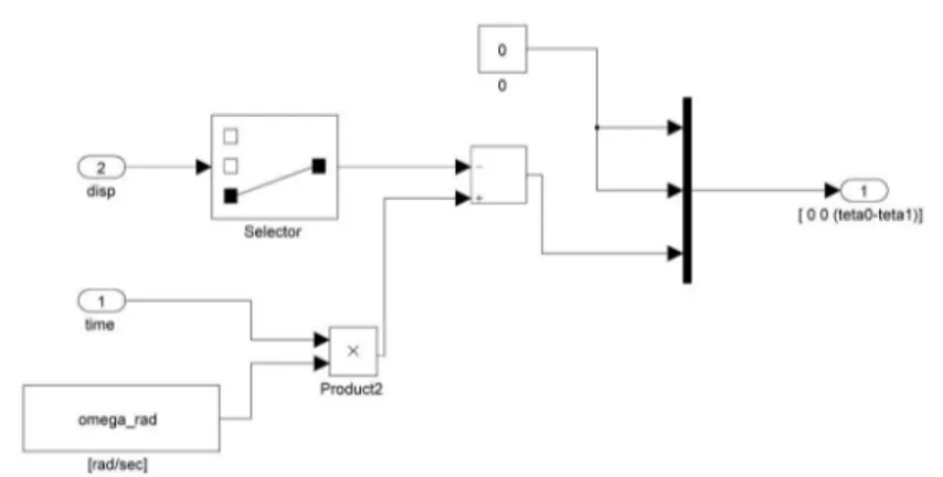
4.1 Simulink flow chart of the rotor shaft equilibrium problem. The model file is called rotor equilibrium look up.mdl. . . 68
4.2 Detail of rotor equilibrium look up.mdl: the integrators. . . 69
4.3 Integration parameters in the Simulink dialog box. . . 69
4.4 Detail of rotor equilibrium look up.mdl: a passage for the motor drive torque calculation. . . 70
4.5 Detail of rotor equilibrium look up.mdl: the periodic time cal-culation. . . 70
4.6 The periodic time calculated by the block of Figure 4.5. . . 71
4.7 The input data for the models (p. 1). . . 72
4.8 The input data for the models (p. 2). . . 73
4.9 The input data for the models (p. 3). . . 74
4.10 The input data for the models (p. 4). . . 75
4.11 The input data for the models (p. 5). . . 76
4.12 The script system 26.m syntax (p. 1). . . 78
4.13 The script system 26.m syntax (p. 2). . . 79
4.14 The script rotor dyn force.m syntax (p. 1). . . 80
4.15 The script rotor dyn force.m syntax (p. 2). . . 81
4.16 The full model.m syntax. . . 82
5.1 The pump P HV 05 on the test bench in normal configuration (on the left) in with the modified cover and measurements devices (on the right). . . 85
5.2 The pump P HV 05 modified to perform experimental measure-ments in working condition. . . 85
5.3 Pressure evolution in the full flow condition in a vane space (solid line) and in a hole control volume (dash-dot line). . . 85
5.4 Pressure evolution in the zero flow condition in a vane space (solid line) and in a hole control volume (dash-dot line). . . 86
5.5 The drainage flow rate (blue line) and the outlet flow rate (red line). . . 86
5.6 Motor torque variation (red line) from the full flow condition to the zero flow condition (see blue line). . . 87
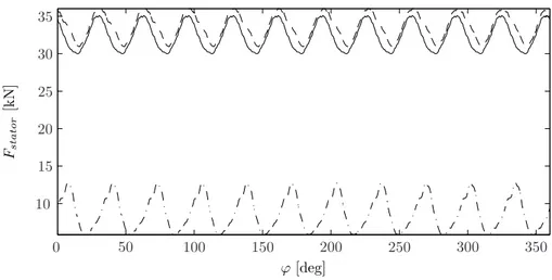
5.7 Radial pressure forces acting on the pump casing. . . 88
5.8 Forces acting on the pressure ring due to centrifugal actions rel-ative to lubricant (Fco,i) and vane (Fcv,i). . . 89
5.9 Force acting on the pressure ring in the full flow condition: x component (solid line), y component (dash-dot line), total force (dashed line). . . 90
5.10 Force acting on the pressure ring in the zero flow condition: x component (solid line), y component (dash-dot line), total force (dashed line). . . 90 5.11 Force acting on the rotor in the full flow condition: x component
(solid line), y component (dash-dot line), total force (dashed line). 91 5.12 Force acting on the rotor in the zero flow condition: x component
5.14 Measurement points on the pressure ring, direction −y (A); on the pressure ring, direction −x (B); on the journal bearing cover
side (C) and on the journal bearing, motor side (D). . . 93
5.15 Detail of accelerometers mounted on the journal bearing, motor side, point D (a) on the pressure ring, −y direction, point A and −x direction, point B (b). . . 94
5.16 Excitation points on the pump casing. . . 94
5.17 Power spectrum density (P SD) of all the hammer blows. . . 94
5.18 The sealing on the rotor shaft hole used to realize the passage of the accelerometers cables. . . 95
5.19 Frequency response function obtained exciting the pump casing in point 1 and measuring the acceleration in point A. . . 95
5.20 The accelerometers placed on the pump casing. . . 97
5.21 Time synchronous average of the acceleration signal acquired in correspondence of point 3 (see Figure 5.20). . . 97
5.22 Frequency spectrum of the time synchronous average signal de-picted in Figure 5.21. . . 98
5.23 Comparison between pressure measured in working conditions (dash-dot line) and pressure calculated by the lumped parameter model (solid line) in the full flow condition for a vane space. . . . 99
5.24 Comparison between pressure measured in working conditions (dash-dot line) and pressure calculated by the lumped parameter model (solid line) in the full flow condition for a hole control volume. . . 99
5.25 Comparison between pressure measured in working conditions (dash-dot line) and pressure calculated by the lumped parameter model (solid line) in the zero flow condition for a vane space. . . 100
5.26 Comparison between pressure measured in working conditions (dash-dot line) and pressure calculated by the lumped parameter model (solid line) in the zero flow condition for a hole control volume. . . 100
5.27 Outlet flow rate evolution in the full flow condition. . . 101
5.28 Drainage flow rate evolution in the full flow condition. . . 102
5.29 Outlet flow rate evolution in the zero flow condition. . . 102
5.30 Drainage flow rate evolution in the zero flow condition. . . 102
5.31 The motor drive torque evolution on a vane pitch in the full flow condition. . . 103
5.32 The motor drive torque evolution on a vane pitch in the zero flow condition. . . 104
5.33 Comparison between the forces acting on the pressure ring in working condition (solid line) and the forces calculated by the LP model (dash-dot line) in full flow condition, x direction. . . . 105
5.34 Comparison between the forces acting on the pressure ring in working condition (solid line) and the forces calculated by the LP model (dash-dot line) in full flow condition, y direction. . . . 105
5.35 Comparison between the forces acting on the pressure ring in working condition (solid line) and the forces calculated by the LP model (dash-dot line) in zero flow condition, x direction. . . 106
working condition (solid line) and the forces calculated by the
LP model (dash-dot line) in zero flow condition, y direction. . . 106
5.37 Position corresponding to 12 deg after the initial position. . . 107
5.38 Comparison between the forces acting on the rotor shaft in work-ing condition (solid line) and the forces calculated by the LP model (dash-dot line) in full flow condition, x direction. . . 108
5.39 Comparison between the forces acting on the rotor shaft in work-ing condition (solid line) and the forces calculated by the LP model (dash-dot line) in full flow condition, y direction. . . 108
5.40 Comparison between the forces acting on the rotor shaft in work-ing condition (solid line) and the forces calculated by the LP model (dash-dot line) in zero flow condition, x direction. . . 109
5.41 Comparison between the forces acting on the rotor shaft in work-ing condition (solid line) and the forces calculated by the LP model (dash-dot line) in zero flow condition, y direction. . . 109
5.42 Pump casing accelerations in correspondence of points 1, 2, 3, 4 of Figure 5.20, full flow condition. The black square markers rep-resent experimental accelerations, while the red circular markers represent the calculated accelerations. . . 113
5.43 Pump casing accelerations in correspondence of points 1, 2, 3, 4 of Figure 5.20, zero flow condition. The black square mark-ers represent experimental accelerations, while the red circular markers represent the calculated accelerations. . . 114
5.44 Comparison between the experimental and the calculated accel-eration relative to point 3, in full flow condition (a) and in zero flow condition (b). . . 115
6.1 Rotor shaft accelerations in full flow condition, along x direction (a) and y direction (b). . . 118
6.2 Control volumes configuration in the angular position correspond-ing to ϕ = 1.7 deg. . . 119
6.3 Control volumes configuration in the angular position correspond-ing to ϕ = 11.5 deg. . . 119
6.4 Control volumes configuration in the angular position correspond-ing to ϕ = 22.2 deg. . . 120
6.5 Control volumes configuration in the angular position correspond-ing to ϕ = 24.5 deg. . . 120
6.6 Control volumes configuration in the angular position correspond-ing to ϕ = 31.4 deg. . . 121
6.7 Rotor shaft accelerations in zero flow condition, along x direction (a) and y direction (b). . . 122
A.1 The outlet control volume shape (V23). . . 127
A.2 The inlet control volume shape (V24). . . 128
A.3 The inner outlet control volume shape (V25). . . 128
A.4 The inner inlet control volume shape (V26). . . 129
B.1 Journal bearing reaction force in the full flow condition. . . 131
List of Tables
2.1 Pump PHV 05 main design features. . . 15
2.2 Pump PHV 05 port plate design data. . . 16
2.3 Pump PHV 05 pressure ring and rotor geometry features. . . 17
2.4 Pump PHV 05 vane geometry features. . . 17
2.5 Pump PHV 05 main clearances values. . . 18
2.6 Lubricant Shel Tellus ST 46 main features. . . 18
3.1 Deflection angle in correspondence of constraints. . . 62
3.2 Finite element dynamic simulation parameters. . . 62
4.1 Initial conditions in terms of displacements and velocities for the integration of the rotor shaft equilibrium problem. . . 69
5.1 Instrumentation used during the F RF measurements. . . 93
5.2 Acceleration measurements in working conditions. . . 96
5.3 Order tracking parameters. . . 97
5.4 PGP values for the pressure evolutions in a vane space and in a hole control volume, for the full flow and zero flow condition (δ = 3%). . . 99
5.5 Drainage and outlet flow rate values. . . 101
5.6 Motor drive torque in full flow and zero flow condition. . . 103
5.7 Comparison between the RM S statistical parameter applied to measured and calculated accelerations signals. . . 112
6.1 Main dynamical phenomena and time when they take place in percentage of the vane pitch. . . 118
List of Symbols
∆ϕ Angular step [deg]ηc Carving slope [deg]
ηvh Vane head slope [mm]
γT Proportional damping factor [s]
µ Lubricant dynamic viscosity [Pa·s]
µf Friction coefficient between vane head and pressure ring inner race
ω Angular velocity [rad/s]
φ Current angular coordinate used to calculate the passage area [deg] ρ Lubricant density [kg/m3]
θc Carving splay [deg]
ϕ Angular coordinate [deg]
ϕ0 Input angular coordinate for the rotor dynamic equilibrium model
ϕtvb Vane angular extension [deg]
ϕvp Vane pitch [deg]
Ai(ϕ) Passage area for control volume i [m2]
Av(ϕ∗) Frontal area of the trapped volume [mm2]
A23,i Exchange area between control volume i and outlet duct [mm2]
A24,i Exchange area between control volume i and inlet duct [mm2]
A25,i Exchange area between control volume i and inner outlet duct [mm2]
A26,i Exchange area between control volume i and inner inlet duct [mm2]
Aduct Area of ducts between internal and external distribution volumes [mm2]
Ainlet Inlet duct interface area [mm2]
bc Carving base width [mm]
bi(ϕ) Meatus width [mm]
bf Width of the meatus between vane flank and port plates [mm]
bhr Width of the meatus between rotor and port plates, starting from hole
control volume [mm]
bh Width of the meatus between vane and rotor groove [mm]
Boil Lubricant bulk modulus [Pa]
br Width of the meatus between rotor and port plates [mm]
bs Width of the meatus between pressure ring and port plates [mm]
Cr Radial clearance in the journal bearing [mm]
CT Test bench shaft proportional damping [Nm/rads]
D Actual displacement [cm3/rev]
db Journal bearing diameter [mm]
dd Duct between internal and external distribution diameter [mm]
e Stator eccentricity [mm]
ef Component of the eccentricity between rotor and pressure ring inner
race due to shaft displacement [mm]
ei Imposed eccentricity between rotor and pressure ring [mm]
esep Component of the eccentricity between rotor and pressure ring inner
race due to journal bearings behavior [mm]
etot Total eccentricity between rotor center and pressure ring inner race [mm]
f Shaft displacement [mm]
fb Journal bearing friction coefficient
Fb,x Journal bearing force reaction in x direction [N]
Fb,y Journal bearing force reaction in y direction [N]
Fco,i(ϕ) Force on the pressure ring due to centrifugal acceleration of lubricant
in control volume i [N]
Ff v,i(ϕ) Force acting on the pressure ring due to the contact force between vane
i and pressure ring [N]
Fhr,i(ϕ) Force acting on the rotor shaft due to pressure in the generic hole i [N]
i [N]
Fstator(ϕ) Force acting on the pressure ring [N]
Fvh,i(ϕ) Contact force between vane i and pressure ring [N]
Fvr,i(ϕ) Force acting on the rotor shaft due to pressure in the generic vane
space i [N]
Fvr,i(ϕ) Force acting on the rotor shaft due to the action of the pressure field
on the generic vane i [N] G Shear modulus [GPa] hc Carving depth [mm]
hd Clearance between rotor and distributor [mm]
hf Clearance between vane flank and port plate [mm]
hg Clearance between a vane and a rotor groove [mm]
hi(ϕ) Meatus thickness [mm]
hp Port plate thickness [mm]
hv Vane heigh [mm]
hhr Thickness of the meatus between rotor and port plates, starting from
hole control volume [mm]
hh Thickness of the meatus between a vane and rotor groove [mm]
Hout,in Frequency response function with input in in and output in out [(m/s2)/N]
hrg Distance between the vane bottom and the rotor [mm]
hr Thickness of the meatus between rotor and port plates [mm]
hs Thickness of the meatus between pressure ring and port plates [mm]
I Polar moment of inertia of the shaft [m4]
i Subscript denoting control volumes
J Rotating parts polar moment of inertia [kg m2]
j Subscript denoting control volume in communication with control vol-ume i
k Flow coefficient
KT Test bench shaft torsional stiffness [Nm/rad]
L(ϕ) Distance between rotor center and stator inner race [mm] lc Carving length [mm]
f
lhr Length of the meatus between rotor and port plates, starting from hole
control volume [mm]
lh Length of the meatus between vane and rotor groove [mm]
lr Length of the meatus between rotor and port plates [mm]
ls Length of the meatus between pressure ring and port plates [mm]
m Rotating parts mass [kg] Mm Motor drive torque [Nm]
Mp(ϕ) Torque due to pressure distribution [Nm]
mv Mass of a vane [kg]
Mvd Torque due to viscous actions [Nm]
Mvh(ϕ) Torque due to friction between vane head and pressure ring [Nm]
N Number of vanes p Pressure [Pa] p∗ Normalized pressure
p0 First trial pressure [Pa]
pdrain Drainage pressure [Pa]
pin Inlet pressure [Pa]
pout Outlet pressure [Pa]
P GP Percentage of good points index [%]
Qi Generic flow rate for the control volume i [m3/s]
Qdrag Drag flow rate for vane spaces [m3/s]
Qdrain Drainage flow rate [m3/s]
Qexp Theoretical outlet flow rate [m3/s]
Qhd Drainage flow rate for holes [m3/s]
Qht Turbulent flow rate between holes and distribution ducts [m3/s]
Qinlet Inlet flow rate [m3/s]
Qlam,i Sum of all the laminar flow rate involved in the ith control volume
bal-ance [m3/s]
[m /s]
Qvd Laminar flow between the rotor and the port plate for a vane space
control volume [m3/s]
Qvf Laminar flow rate on a vane flank [m3/s]
Qvh Laminar flow rate from a vane space to a hole [m3/s]
Qvs Drainage flow between the pressure ring and port plates [m3/s]
Qvt Turbulent flow rate from a vane space to distribution ducts [m3/s]
Rb Beraring radius [mm]
rc External duct carving radius [mm]
re External ducts radius [mm]
ri Internal ducts radius [mm]
rp Duct end fillet radius [mm]
rr Rotor radius [mm]
rs Shaft radius [mm]
rf rg Fillet radius at the end of a rotor groove [mm]
rhr Hole radius [mm]
ric Internal duct carving radius [mm]
rse Pressure ring external radius [mm]
rsi Pressure ring inner radius [mm]
rsr Rotor side radius [mm]
SEP Journal bearing static equilibrium position [mm] tvb Vane base thickness [mm]
tvh Vane head thickness [mm]
temp Lubricant temperature [◦C]
u Tangential velocity [m/s] Vh Generic hole volume [m3]
Vi Generic control volume
vs Journal bering squeeze velocity [m/s]
Vv Generic vane volume [m3]
c
Wp Rotor and pressure ring common width [mm]
Wr Rotor width [mm]
Ws Pressure ring width [mm]
Wv Vane width [mm]
Wsr Rotor side width [mm]
x Rotor shaft degree of freedom corresponding to horizontal direction y Rotor shaft degree of freedom corresponding to vertical direction z Rotor shaft degree of freedom corresponding to axial direction
Introduction
In this introductory section a general overview of the present study will be pro-vided. Dealing with high pressure variable displacement vane pumps great at-tention must be payed to all the dynamic phenomena taking place inside such machinery. For this reason several advanced modeling techniques have been de-veloped and used. The basic theory, the applications and the results of these models will be reported in the present work following the scheme underlined hereafter.
1.1
Variable displacement vane pumps
peculiar-ities
Vane pumps are a particular kind of positive displacement pumps (P D), in which a unit of fluid is physically transferred from an inlet region to an out-let region. In the family of P D pumps, vane pumps can be classified as ro-tary pumps. With respect to alternative pumps, this category will produce a smoother and more continuous flow, while alternative pumps will lead to a pulsed flow. Between vane pumps it is possible to distinguish three subfamilies [1]:
• Single chamber vane pumps: they uses an eccentric circular pressure ring that allows to obtain for each vane space a single cycle from inlet to outlet pressure per rotor revolution;
• Double chamber vane pumps: they uses an elliptical pressure ring charac-terized by a double eccentricity that allows to obtain for each vane space a double cycle from inlet to outlet pressure per rotor revolution;
• Variable displacement vane pumps: in this kind of vane pumps a circular pressure ring can vary his eccentricity with respect to the rotor shaft. The three items previously listed are respectively depicted in Figures 1.1, 1.2, 1.3, where the inlet region is represented in blue, while the outlet region in red. The pump studied in this thesis is a variable displacement high pressure vane pump. This kind of P D pump is widely used in machine tools and in hydraulic systems thanks to its control strategy. In fact the lubricant flow rate can be
Figure 1.1: Single chambre vane pump.
Figure 1.2: Double chambre vane pump.
simply tuned accordingly to system and efficiency requirements by varying the relative eccentricity between pressure ring and rotor shaft. In this way the pump elaborates only the required flow rate allowing to save energy. This main feature leads to select a variable displacement vane pump for all the applications in which the plant needs to be kept at working pressure by compensating the plant losses and only occasionally a flow rate is required to move tools mounted on the lyne. This is the typical case of a machine tool, i. e. a drill, that usually stands still, only when the tool start to be used the variable displacement vane pump starts to elaborate the required flow rate. As a machine tool component, the pump being studied must provide low vibration and acoustic levels to ensure high working precision as well as health and comfort of technicians. In this sight, an optimization process must be performed to reduce vibration levels and noise emissions. This optimization process is based on advanced modeling techniques as described hereafter.
1.2
Modeling mechanical systems
Modeling a complex mechanical system is often an hard task, in fact a complete knowledge of the system is required to avoid mistakes and errors, a coherent for-mulation of the problem must be done and finally the mathematical forfor-mulation must be implemented in an efficient and smart way. Let us consider separately all this step resumed in the flow chart of Figure 1.4 [2]. In more detail, the mechanical system to be studied will be analyzed in Chapter 2, the physical
Figure 1.3: Variable displacement vane pump.
Figure 1.4: Flow chart of an ideal modeling process.
model and the mathematical formulation will be treated in Chapter 3, the main aspects of the implementation will be described in Chapter 4, the validation procedure will be reported in Chapter 5 and finally an example of application will be summarized in Chapter 6.
1.2.1
Physical model
Usually the physical model represents an equivalent system of the actual me-chanical system under some hypotheses:
• The distributed characteristics (e.g. density, stiffness, damping, etc) are replaced with lumped characteristics;
• When possible the system behavior is supposed to be linear;
• The system parameters are not time-varying;
• The uncertainties are neglected.
The physical model built up depends on the kind of analysis that has to be performed. For example to study the pump PHV 05 a kyneto-elastodynamic model has been developed. Using such an approach, the properties of the system in terms of mass, stiffness and dumping are considered as Lumped Parameters, for this reason it is called LP model.
1.2.2
Mathematical model
This kind of LP model can be generally represented by means of the second order system of differential equations (1.1):
[M ]¨x + [C] ˙x + [K]x = F (t) (1.1)
where [M ], [C] and [K] represents the mass, the viscous damping and the stiff-ness of the system and F (t) is the external force field applied to the system, while ¨x, ˙x and x are respectively the vectors of accelerations, velocities and displacements.
In the case of volumetric pumps, the force calculation can be generalized as stated in equation (1.2), where si is the generic surface in which the pressure pi
is acting.
Fi=
"
pidsi (1.2)
For this reason a deep characterization of the pressure field is required because quantity F (t) in equation (1.1) can be determined once the pressure evolution around the rotor shaft is calculated. The pressure field calculation involves the solution of a first order differential equation system whose equations can be written in a general way as follows:
dpi
dϕ = f (p) (1.3)
Where pi represents the pressure evolution in a generic control volume and p
represents the whole pressure field to be calculated.
1.2.3
Integration
The system of first order differential non linear equations, with non constant coefficients describing the pressure field is an example of stiff problem. To solve it, a variable order solver, based on the numerical differentiation formulas (NDFs) has been used. The algorithm is an explicit Runge-Kutta variable step formulas for stiff initial values problems (IVPs) [3]. On the other hand, dealing with the rotor shaft equilibrium system solution, also fixed step solvers can be used. In this case the solution is easier and faster because the problem is non-stiff and it is described by few equations.
1.3
Variable displacement vane pump: state of
the art and modeling
When dealing with variable displacement vane pumps, the use of models is suit-able to investigate and optimize several aspects related to working condition. In particular, since this kind of pumps often equips machine tools, great im-portance is given to the optimization of the vibrational behavior to ensure high working precision as well as comfort of technicians.
The first step in order to simulate the pump dynamic behavior is the develop-ment of a dynamic model of the rotating parts. A Lumped Parameter (LP )
model is generally considered for this purpose: this approach consists in con-sidering all the inertia, the stiffness and the damping properties as lumped. An example of this method applied to gear pumps can be found in [2, 4–6] that are taken as starting point in this study. Then, once the loads in terms of pressure forces and torques are known, it is possible to integrate the equations of motion obtaining the rotating part accelerations as well as the bearing force reactions. In the above mentioned works, these bearing reactions are calculated by a non linear algorithm based on the finite impedance theory [7].
As stated before, the determination of loads in terms of pressure forces and torques is required for the integration of the equations of motion involved in the LP model of the rotor shaft equilibrium. These loads are a function of the pressure field inside the pump that is the first aspect to be studied in a proper pump modeling process. As a matter of fact, all the variable forces acting on the pump casing are due to variations in the pressure field. Hence in the frame of a noise and vibration optimization the reduction of pressure ripple is crucially important because this phenomenon generates variable forces and finally body vibrations. An attempt to investigate and minimize the ripple phenomena has been described by Hattori et al. [8]. This work is based on the study of the pump by means of an Euler’s approach, as proposed in [9– 13]. Using this modeling technique, the pump fluid domain is divided in several control volumes; hence, the flow rate continuity equation can be applied to each control volume. The pressure field and the flow rates that characterize the pump can be finally obtained by integrating the system of flow rate continuity equations.
Once the pressure field is determined, it is possible to calculate the main exci-tation forces that load the pump components. Dealing with this fundamental calculation, several works have been performed by Fiebig and Heisel [13], Manc`o et al. [14], Gellrich at al. [15] and Novi et al. [16]. In all the above mentioned works, the force calculation is performed to study wear phenomena taking place inside the pump and mainly deals with the calculation of contact forces between the vane head and the pressure ring.
Another important step in modeling a variable displacement vane pumps is the validation procedure used to assess the pressure evolution basing on the comparison between calculated pressures and pressures measured in working condition. Works dealing with this topic have been carried out by Bianchini et al. [17] and Kunz et al. [18].
The results in terms of pressure loads can be combined with frequency response functions (F RF s) of the pump casing to calculate the casing accelerations that are the main sources of noise and vibrations. In this way the operational acceler-ations of the casing can be obtained and compared with acceleracceler-ations measured in working condition to validate the whole procedure. Such an approach has been used from an acoustical point of view by Dickinson et al. [19]. In a more similar way the same validation method has been exposed by Mucchi et al. in [20], in which F RF s simulated by means of a finite element model have been used instead of experimental F RF s.
In this context, this works aims at developing tools useful to carry out a noise and vibration optimization by considering all the approaches underlined in the state of the art outlined above. In more detail, the model developed in this thesis can be used for the analysis of the dynamic behavior of the rotor shaft. It is a simple, but non-linear, model taking into account only the transversal
plane dynamics of the rotor shaft. In addition to the pressure forces and torque, the dynamic equilibrium of the rotor shaft includes the non-linear reactions of the hydrodynamic journal bearings, the torsional stiffness and damping of the driving shaft, as well as the friction effects. This model allows to simulate the rotor shaft accelerations, the journal eccentricity and the time variable reactions in the bearings in working condition.
As stated before, the LP model includes the evaluation of pressure forces and torques. These quantities are functions of the pressure field, for this reason an algorithm based on an Euler’s approach has been developed as well. This algorithm studies the pressure field by dividing the pump fluid domain in several control volumes, hence the flow rate continuity equation can be applied to each control volume. The results of the pressure calculation can be compared with experimental pressure evolution to carry out a first validation.
The assessed pressure evolutions can be used as input data for subroutines devoted to variable pressure forces and torques calculation. These last results are used by the above mentioned LP model to integrate the rotor shaft equations of motion to finally calculate the journal bearing reaction forces as well as the rotor shaft accelerations and the journal bearing eccentricity in working condition. Moreover, the variable pressure and bearing forces evaluated by means of the LP model have been combined with frequency response functions of the pump casing, experimentally estimated. In this way the operational accelerations of the casing can be obtained and compared with accelerations measured in work-ing condition to validate the whole procedure.
Finally, once the LP model can be considered validated, a study on the calcu-lated rotor shaft acceleration can be performed with the aim at studying the dynamical phenomena related to pump working condition.
All the algorithm useful to carry out the calculations related to the modeling process outlined in the present section have been developed in MATLAB and Simulink environments. The experimental data used for comparisons and vali-dations have been acquired and processed by means of LMS Test.Lab.
1.4
Overview of the thesis
In order to achieve the goals listed above (analysis of the behavior of the system, evaluation of the dynamic forces, etc.) the model described in the previous section has been developed and experimentally assessed.
The first step in a proper modeling activity is the full knowledge of the compo-nent being studied. For this reason a general description of variable displacement vane pump has been reported in Chapter 2. Hence a complete characterization of pump PHV 05 produced by BERARMA s.r.l (Casalecchio di Reno, Bologna, Italy) has been provided from a geometrical and operational point of view. In this frame great attention has been payed for the components involved in pump working. The port plate geometry has been fully characterized, hence the rotor, the vane and the pressure ring main dimensions have been provided. Furthermore, the clearances between pump components have been determined, whose geometrical features will influence the communications between the con-trol volumes used to compute the pressure evolutions. Finally the lubricant main features have been specified. The model developed in the present work will use as inputs all these data.
In Chapter 3 the LP model is presented in depth from a theoretical point of view. First of all the general features of the model are exposed starting from the system of equation of motion that governs the rotor shaft equilibrium. Hence the calculation of all the quantities involved in the system integration is described. In this frame the procedure for pressure evolution calculation is deeply analyzed. This procedure is based on an Euler’s approach that allows to determine the pressure field by integrating a system of flow rate continuity equations, each one referred to the control volumes used to discretize the whole fluid domain. Once the pressure evolution has been determined, the variable pressure forces acting on the rotor can be calculated. Hence, the journal bearing reaction forces can be determined basing on the finite impedance formulation. The calculation of torques acting on the rotor shaft has been described as well. Three kind of load torques have been considered: torques due to the pressure evolution inside control volumes; torques due to the friction between the vanes and the pressure ring and torques due to viscous actions. In this sense, the developed lumped parameter model takes into account the most important phenomena taking place inside the pump in working conditions, most of them are non linear and time varying. Finally, for the sake of completeness, a preliminary analysis is reported to asses the goodness of the assumptions used to develop the model.
In Chapter 4 the main problems related to model implementation in MATLAB and Simulink are described and the most interesting code pieces are reported as well. In this frame the integration of the equations of motion characterizing the rotor shaft equilibrium is carried out in Symulink. The whole model has been described with reference to the blocks that constitutes itself. In more detail, the initial conditions choice has been discussed, and the integration strategy as well as the interface between Symulink and MATLAB are explained by means of images depicting the blocks architecture. The main aspects related to the implementation in MATLAB of the subroutines devoted to the pressure evolu-tion, the pressure forces and the torques calculations are discussed. The most interesting pieces of code are attached as well.
In Chapter 5 the method used to assess the LP model has been exposed. First of all the measurements performed during the test campaign have been described. A suitably modified pump has been used to measure the pressure evolutions in working condition in all the regions of interest. Tests at different work-ing pressures have been carried out to evaluate the flow rates and the motor drive torques in different working conditions. The method used to calculate the pressure forces from the pressure measurement has been explained, hence, the original procedure used to measure the frequency response functions of the pump casing is reported. Finally, the casing accelerations measurements and processing is briefly explained. The above mentioned experimental data have been used to assess the model. The validation procedure has been carried out on several levels, in this way the goodness of intermediate results is checked as well. In more detail, the calculated pressure evolution has been assessed by using the experimental pressures. The same validation strategy has been applied to vali-date the flow rates and the torques. Subsequently, the pressure forces calculated by means of an ad hoc method applied to experimental and calculated pressures have been compared and discussed. Hence, the above mentioned forces have been combined with the frequency response functions to calculate the pump casing accelerations. This last results is finally assessed by comparison with the experimental accelerations and the results have been discussed as well.
Since the model can be considered globally validated, in Chapter 6 an example of application has been provided. The results in terms of rotor shaft accelerations are used to establish the events related to unwanted dynamical effects. The analysis has been carried out in the two main working conditions.
The final considerations about the whole modeling and experimental activity are finally reported in Chapter 7, devoted to concluding remarks.
Moreover in Appendix A the volume amount and shape of inlet and outlet control volumes are resumed and in Appendix B the journal bearing reaction forces are reported.
General description of a
variable displacement vane
pump
The hydraulic pump universe includes a wide choice of volumetric pumps. In this frame it is possible to classify pumps by using several criteria, such as the pressure range in which they work, the way used to obtain the desired displace-ment, the possibility to vary the displacement. This chapter will focus on the high pressure variable displacement vane pump family, in particular a pump of the series PHV by BERARMA oleodinamica will be fully described. An analysis of the working condition will be provided as well to fully understand the present work.
2.1
Vane pump basic description
A lot of different classifications can be done when dealing with hydraulic pumps [21]. A first classification is based on the working principle and it is shown in Figure 2.1: the dynamic pumps give energy to the flow by imparting a velocity amount able to transfer the flow rate from the inlet to the outlet, while pumps based on positive displacement traps a fluid volume and physically move it from the inlet to the outlet. Vane pumps belong to the latter category: they are composed by a cast iron body in which a one piece rotor shaft, a pressure ring and two port plates are located. The pressure ring is eccentric with respect to the shaft axis and in this way the volume isolated between two consecutive vanes varies from a maximum value, in correspondence with the inlet port, to a minimum value, in correspondence with the outlet port. Vane pumps with a double pressure chamber can be realized using an elliptical pressure ring and can transport fluid from inlet to outlet two times per revolution. Vane pumps with circular pressure ring have only one pressure chamber and are widely used. Both this kind of vane pumps can not vary their actual displacement in working condition.
Variable displacement van pumps can supply to this task by varying the relative eccentricity between rotor and pressure ring (stator): they can elaborate a full
Figure 2.1: Vane pumps sorting.
(a) (b)
Figure 2.2: The two extreme working conditions: full flow (a) and zero flow (b).
flow rate (see Figure 2.2(a)) till the desired pressure level is reached, or they can work in a zero flow condition (see Figure 2.2(b)), just to keep the desired pressure by compensating the hydraulic losses. While the full flow condition is characterized by the maximum eccentricity between rotor and stator, in the zero flow condition there is almost no eccentricity.
The variable displacement vane pump main elements are depicted in Figure 2.3 [22]. The control piston (6) moves the pressure ring changing the pump actual displacement, the bias piston (7) reports the pressure ring in the zero eccentricity condition when the desired pressure level is reached, the balancing screw (5) is used to compensate the main component of the resulting pressure force. The control piston force can be regulated by a tuning screw (8). This mechanical control system can be substituted by an equivalent hydraulic system, called pressure device compensator, depicted in Figure 2.4 [23], in which the control piston (2) and the bias piston (3) act on the pressure ring (1) with a
Figure 2.3: Variable displacement vane pump main components: casing (1), one piece rotor shaft (2), vane (3), pressure ring (stator) (4), balancing screw (5), control piston (6), bias piston (7), tuning screws (8, 9).
force regulated by the lubricant pressure in the inlet and outlet ducts. In fact, the bias piston is always loaded by the outlet pressure. In the start up phase the control piston is loaded by the outlet pressure as well and his resulting force is bigger than the bias piston one, so it can move the pressure ring to his maximum eccentricity (see Figure 2.4(a)) till the desired pressure level is reached. The compensator spring (5), if compressed, allows the communication between the inlet chamber and the control piston (see Figure 2.4(b)). In this last configuration, the bias piston force is bigger then control piston force and the pressure ring is moved again to zero flow condition: the desired pressure level can now be maintained by using a small power amount.
The characteristic curve of a variable displacement vane pump depicted in Figure 2.5 shows that the maximum eccentricity, corresponding to full flow condition, is maintained till the cutoff pressure is reached [24]. The small slope of the first part of the curve is due to hydraulic losses. Once the cutoff pressure is reached, the eccentricity (and the flow rate) and the slope of the second part of the curve are determined by the spring stiffness. This procedure can be reversed when the working pressure decreases under the cutoff value. Finally, it can be noticed from Figure 2.5 that the cutoff pressure and the dead head pressure have almost the same value.
When dealing with vane pumps, one of the most important features is the actual displacement : the lubricant volume transferred from inlet to outlet during a revolution of the rotor shaft. It is a function of the volume that each vane space traps after the end of inlet ducts and before the beginning of the outlet ducts. It can be calculated as stated in equation (2.1).
D = Av(ϕ∗)N Wr (2.1)
Where, the quantity Av(ϕ∗) represents the frontal surface of the trapped vane
space at the angular position ϕ∗, N is the number of vanes and W
r is the rotor
width in axial direction. The volume of the trapped vane space depends on design parameters such as external rotor diameter, rotor width in axial direction,
(a)
(b)
Figure 2.4: The pressure device compensator in full flow condition (a) and in zero flow condition (b).
Figure 2.5: Variable displacement vane pump characteristic curve.
Figure 2.6: Angular coordinate at the beginning of the trapped volume
inner pressure ring diameter, and on the eccentricity between rotor and pressure ring. The procedure to calculate D consists in determining the evolution of the vane space surface during a revolution (Av), then it is easy to evaluate
the quantity Av(ϕ∗). The angular coordinate ϕ∗ is determined as the angular
coordinate in which the first vane with respect to the angular velocity ω (i.e. V11 in Figure 2.6) passes the inlet duct.
When the design of distributors is unknown, a less accurate estimation of ac-tual displacement can be obtained by considering the trapped vane space as a rectangular surface in correspondence of the maximum eccentricity (emax).
D = 2πrmemaxWr (2.2)
In equation (2.2) rmrepresents the mean radius between the eternal rotor radius
and the radius of the inner race of pressure ring, while Wr represents the rotor
width along the axial direction. In this way the displacement is overestimated. The actual displacement depends also on the trapped volume sealing, useful to avoid hydraulic losses inside the pump. The sealing is guarantee by the centrifugal force and by an amount of lubricant at outlet pressure in the vane housing (corresponding to rotor holes). The force acting between the stator inner race and the vane head must be controlled to avoid excessive wear and the contact surface must be designed as well. For this reason a lot of solutions have been proposed, in Figure 2.7 two widely used vane designs are depicted [25].
(a) (b)
Figure 2.7: Two typical designs for the vane-stator coupling: an old solution (a) and a new solution to minimize wear due to the contact between the vane head and the stator (b).
2.2
BERARMA
PHV 05 pump
2.2.1
Overview
The pump under study is made by BERARMA oleodinamica (Casalecchio di Reno, Bologna, Italy) and belongs to the PHV family. The model being studied is the PHV 05 [26]: it is an high pressure variable displacement vane pump that take advantage of a double inlet/outlet port plate system in which each port is packed on the pressure ring by using a system based on hydrostatic compensation. Such a pump uses a pressure device compensator (described in section2.1) to vary his actual displacement. The main component shown in Figure 2.3 can now be identified on the PHV 05 pump (see Figure 2.8, 2.9 and 2.10).
To fully describe the pump PHV 05, the flow rate characteristic curve and the drainage flow rate range are provided in Figure 2.11 and 2.12.
2.2.2
PHV 05 design parameters
Before describing the mathematical formulation of the model (see next chapter), it is useful to define the geometry of the vane pump and the reference frame used. The displacement of the rotor in axial direction has been neglected as well as the pressure variation in axial direction. Therefore the geometry taken into account is a plane geometry, orthogonal to the shaft axis direction. Nevertheless, to avoid misunderstanding it is important to impose a 3-dimensional coordinate system (see Figure 2.8 and 2.9): the z axis identifies the shaft direction, while the xy plane defines a rotor shaft cross section. The angular coordinate ϕ start to be computed in correspondence of the −y axis, with positive verse in the angular velocity direction. The main design data are listed in table 2.1 [26]. The port plate design is crucially important in determining a proper pump behavior. Figure 2.13 and 2.14 depict the meaning of the most important design parameters and Table 2.2 resumes their values.
As stated in section 2.1, in this kind of pumps the actual displacement as well as the outlet flow rate can be defined with respect to rotor and pressure ring geometry, respectively depicted in Figure 2.15 and 2.16, whose main geometrical features are defined in 2.3.
Figure 2.8: Pump PHV 05 main components.
Table 2.1: Pump PHV 05 main design features. Actual displacement (ISO 3662) 16 cm3/rev
Max working pressure allowed 250 bar Max drainage pressure allowed 1 bar Inlet pressure (pin) 0.8 ÷ 1.5 bar
Rotational velocity 1350 ÷ 1500 rpm
Finally, to fully define the main components, the vane geometry has to be characterized (see Figure 2.17 and Table 2.4).
To complete the geometry description, also the geometrical clearances have to be taken into account. This aspect is capitally important when dealing with high pressure pumps because the flow rates taking place inside the clearances are not negligible in a proper model construction. Table 2.5 resumes the main clearances values.
The pump P HV 05 has been tested using the lubricant Shel Tellus ST46 whose main features are reported in Table 2.6
For the sake of completeness in Appendix A, the distribution ducts are charac-terized in terms of shape and volumes.
2.3
Working condition description
This kind of pump is widely used for applications in machine tools tanks to the possibility to regulate the flow rate accordingly to the system requests. In this way it is possible to minimize hydraulic losses by elaborating only the strictly necessary flow rate. Such a machine typically needs to be kept at working pressure also when there is no request of torque and motion. In this case the variable displacement vane pump works in zero flow condition (see Figure 2.2(b))
Figure 2.9: Pump PHV 05 cross section.
Table 2.2: Pump PHV 05 port plate design data.
hc Carving depth 3.5 mm
θc Carving splay 60 deg
bc Carving base width 0.2 mm
ri Internal ducts radius 18.7 mm
re External ducts radius 25.8 mm
rp Duct end radius 1.75 mm
ϕseo External outlet start angle 28 deg
ϕeeo External outlet end angle 168 deg
ϕsei External inlet start angle 203 deg
ϕeei External inlet end angle 353 deg
ϕsio Internal outlet start angle 343 deg
ϕeio Internal outlet end angle 194 deg
ϕsii Internal inlet start angle 225 deg
ϕeio Internal inlet end angle 330.5 deg
just to compensate the circuit hydraulic losses. When the torque and motion are needed to accomplish the work, the compensator device automatically moves the pressure ring generating the displacement needed to supply the request, till the full flow condition (see Figure 2.2(a)). Of course the pump can work also in intermediate conditions when the pressure ring eccentricity value is less than the biggest allowed. Nevertheless, Figure 2.5 shows that intermediate working conditions are negligible because of the fast passage from the cutoff pressure to the dead head pressure. For this reason the tests have been carried out mainly in full flow or zero flow condition.
To study the working condition behavior, a test bench has been used (see Fig-ure 2.18). The experimental rig allows to measFig-ure the pressFig-ure inside a vane space and inside a hole for a complete shaft rotation by means of piezoelectric transducers directly placed on the one piece rotor shaft. To do this, a suitably designed rotor shaft is used (see Figure 2.19) in which two meatus connect a vane space and a hole to the end of the shaft, where two pressure transducers
Table 2.3: Pump PHV 05 pressure ring and rotor geometry features.
Wr Rotor width 20 mm
rr Rotor radius 27.5 mm
rhr Hole radius 18.3 mm
rsr Rotor side radius 25.5 mm
Wsr Rotor side width 4.5 mm
Ws Pressure ring width 20 mm
rse Pressure ring external radius 86.5 mm
rsi Pressure ring inner radius 30 mm
Table 2.4: Pump PHV 05 vane geometry features.
hv Vane heigh 8.8 mm
Wv Vane width 20 mm
tvh Vane head thickness 0.2 mm
tvb Vane base thickness 2.2 mm
ηvh Vane head slope 30 deg
are placed. The pump cover must be modified as well to allow the rotor shaft passage and finally, two measure chamber are isolated by using O-ring gaskets. The pressure signals and the trigger are acquired and processed by a LMS Scadas SC305 Front-end controlled by software LMS Test-Lab. The pressure sensors being used are piezoelectric transducers Kistler, model 6207, the proximity sen-sor used as trigger is a Balluff BES 516324S4C finally, a charge amplifier Kistler 5006 and an oscilloscope Fluke 96 B Series II, with a sampling frequency of 60 MHz have been used to perform an on-line control of the measurement proce-dure. The torque signal can be acquired as well by a torque transmitter Stiger Mohilo 0160 DM, with a full scale of 500 Nm.
With this set up the measure of the pressure inside a hole and a vane space can be obtained. The results are shown in Figures 2.20 and 2.21, in which the passage from the inlet to the outlet region can be immediately distinguished and the ripple phenomena for the high pressure region are underlined as well. The reference system used to plot the pressure evolution in Figure 2.20 is depicted in Figure 2.9: the angular coordinate reference starts from −y direction. For the sake of completeness also the test bench power train is depicted in Figure 2.18. All these aspects will be deeply analyzed in section 5.2.
Table 2.5: Pump PHV 05 main clearances values.
hf Clearance on the vane flank 0.0173 mm
hd Clearance between rotor and distributor 0.023 mm
hg Clearance between a vane ad a rotor groove 0.0162 mm
Table 2.6: Lubricant Shel Tellus ST 46 main features.
Lubricant viscosity (µ) 11 ÷ 68 cSt
Max lubricant viscosity during start-up 400 cSt Working condition temperature (temp) +15 ÷ +60◦C
Max lubricant contamination allowed 20/18/15
Figure 2.11: Pump PHV 05 characteristic curve.
Figure 2.13: Port plate design.
Figure 2.15: The rotor design.
Figure 2.16: Pressure ring cross section. .
Figure 2.17: The vane design. .
Figure 2.18: The test bench apparatus. .
ϕ [deg] p [b a r] 0 50 100 150 200 250 300 350 0 50 100 150 200 250
Figure 2.20: The pressure measured in a vane space (solid line) and in a hole (dash-dot line) for a complete shaft rotation in the full flow rate condition corresponding to the cutoff pressure.
ϕ [deg] p [b a r] 0 50 100 150 200 250 300 350 0 50 100 150 200 250
Figure 2.21: The pressure measured in a vane space (solid line) and in a hole (dash-dot line) for a complete shaft rotation in the zero flow rate condition, corresponding to the dead head pressure.
Model description
The need to increase the knowledge on the dynamic behavior of a mechanical system leads to the formulation of reliable physical models, from which mathe-matical models can be obtained. After this step the model can be validated by comparing its results with empirical observations and finally the validated model can be used to perform simulations and make predictions.
3.1
General description of the model
The model takes into account only the transversal plane dynamics of the rotor shaft: it is a planar model with 3 degrees of freedom as presented in Figure 3.1. The inertia properties of the rotor shaft is considered to be lumped in the rotor portion carrying the vanes (indicated with ”r” in Figure 3.1). Therefore the degrees of freedom are the displacement along the x and y direction and the angular displacement ϕ of the rotor portion.
Figure 3.1: Model for the dynamic analysis of the rotor shaft.
The known model input is the coordinate ϕ0, representing the angular
displace-ment of the rotor shaft section in which the shaft is joined to the electrical motor drive through a key (see Figure 3.1, shaft portion 1). This section, as well as the motor, is assumed to rotate at constant speed ˙ϕ0. Coordinate ϕ0is
![Figure 3.19: Passage area at the beginning of duct constant area region. ϕ [deg]A1[mm2]050100150 200 250 300 35005101520253035](https://thumb-eu.123doks.com/thumbv2/123dokorg/4739718.46468/73.892.214.602.228.552/figure-passage-area-beginning-duct-constant-area-region.webp)