Exact Distributed Load Centrality Computation:
Algorithms, Convergence, and Applications
to Distance Vector Routing
Leonardo Maccari
∗, Lorenzo Ghiro
†, Alessio Guerrieri
‡, Alberto Montresor
†, Renato Lo Cigno
§∗
University of Venice,
†University of Trento,
‡SpazioDati srl,
§University of Brescia
F
Abstract—Many optimization techniques for networking protocols take
advantage of topological information to improve performance. Often, the topological information at the core of these techniques is a cen-trality metric such as the Betweenness Cencen-trality (BC) index. BC is, in fact, a centrality metric with many well-known successful applications documented in the literature, from resource allocation to routing. To compute BC, however, each node must run a centralized algorithm and needs to have the global topological knowledge; such requirements limit the feasibility of optimization procedures based on BC. To overcome restrictions of this kind, we present a novel distributed algorithm that requires only local information to compute an alternative similar metric, called Load Centrality (LC). We present the new algorithm together with a proof of its convergence and the analysis of its time complexity. The proposed algorithm is general enough to be integrated with any distance vector (DV) routing protocol. In support of this claim, we provide an implementation on top of Babel, a real-world DV protocol. We use this implementation in an emulation framework to show how LC can be exploited to reduce Babel’s convergence time upon node failure, without increasing control overhead. As a key step towards the adoption of centrality-based optimization for routing, we study how the algorithm can be incrementally introduced in a network running a DV routing protocol. We show that even when only a small fraction of nodes participate in the protocol, the algorithm accurately ranks nodes according to their centrality.
Index Terms—Multi-hop networks; Mesh networks; Ad-hoc networks;
Bellman-Ford; Load centrality; Distributed Algorithms; Failure recovery
1
I
NTRODUCTIONTopology awareness enables significant optimizations for dis-tributed systems. For example, the influence of nodes placed in strategic locations can be measured, and these measurements can guide the optimal allocation of resources in the system. In this regard, centrality metrics are well-known instruments provided by graph theory to quantify the influence of the nodes in a network. Among the multitude of centrality indexes proposed in the literature, a widely used one is the Betweenness Central-ity (BC) index: roughly speaking, BC measures the fraction of This work has been partially funded by the European Commission, H2020-ICT-2015 Programme, Grant Number 688768 ’netCommons’ (Network Infras-tructure as Commons) and the H2020 GA No. 645274 “Wireless Software and Hardware platforms for Flexible and Unified radio and network controL (WiSHFUL)" with the project “Pop-Routing On WiSHFUL (POPROW)" fi-nanced in Open Call 3. Lorenzo Ghiro PhD grant is partially supported by the IEEE Smart Cities Initiative at Trento. This paper revises and extends a paper presented at IEEE INFOCOM in 2018 [1], by studying the behavior of the protocol under partial information. This work was initiated when all the authors were with the University of Trento
global shortest paths passing through a vertex [2]. BC has found numerous applications in distributed systems, where it is used for optimal service placement [3], to improve routing [4–6], for topology control [7, 8], for security [9, 10], and for several other uses [11, 12].
We focus on a particular application of centrality in computer networks, namely on the tuning of control messages for faster routing convergence [4]. The idea is to increase the frequency of control messages for the most central nodes while reducing it for marginal ones: this leads to faster re-routing and reduced traffic loss upon an average failure in the network, without increasing the overall control overhead. This tuning technique based on BC has been initially applied only to link-state (LS) routing protocols, as these protocols enable each router to collect information about the full network topology, which is a requirement for the computation of BC [6, 13]. In distance-vector (DV) routing protocols, instead, routers are not required to know the entire topology. This enables networks managed by a DV protocol to scale up to millions of nodes, but does not provide enough information to routers to compute BC. As a consequence, the lack of an exact distributed algorithm is still preventing the centrality-based optimization of DV protocols.
In this paper we target another centrality metric, called Load Centrality (LC) [2, 14], that is very similar to BC, but can be computed in a distributed way. Instead of relying on the number of shortest paths, LC estimates the amount of traffic that insists on a node, assuming that the traffic is fairly distributed among all shortest paths of the network. LC converges to BC in many real-world cases, and we claim that in the rest of the cases LC is a better metric than BC to measure the communication traffic in today’s computer networks and should therefore be preferred for distributed applications. We better detail this claim in Sec. 2.3.
The core of our contribution is the proposal of an efficient dis-tributed algorithm able to exactly compute LC, paving the way for centrality based optimizations in distributed systems. It is defined on top of the Bellman-Ford algorithm, thus can be integrated into any DV routing protocol introducing minimal modifications. The convergence time of our algorithm scales linearly with the network diameter D: after a number of steps bound by 3D, every vertex knows its own centrality and the centrality of all the other vertices. One critical step to go from a sound theoretical approach to a real-world application is the study of the applicability of the algorithm to real protocols. In this paper, we address this problem by studying how the distributed algorithm can be incrementally deployed in an existing network updating a running protocol.
We also show that the estimation of LC is possible when only a subset of nodes in the network supports the updated protocol. This is essential in real protocol deployments: as the network size grows, it becomes less and less feasible to simultaneously upgrade all of the nodes in that network. We provide a mathematical characterization of the approximation errors as a function of the penetration rate for both the centrality estimates and the centrality rankings, and we show that, even with low penetration rate, our algorithm ranks nodes accurately. Finally, we provide simulations that confirm our theoretical findings.
To further show the practical applicability of our contribution, we extend babeld, the open-source implementation of the widely used DV routing protocol for mesh networks specified in RFC 6126 [15]. We show that, exploiting the notion of LC, the protocol convergence time can be improved up to 13% without increasing signaling overhead.
2
B
ACKGROUND ANDC
ONTRIBUTIONSCentrality measures have been used to enhance traffic monitor-ing [5, 9], intrusion detection [16], resource allocation [11] and topology control [7]. Among all, Betweenness Centrality (BC) is a well-known centrality index, which can be computed with Brandes’ centralized algorithm [17]. Brandes’ algorithm executes an instance of Dijkstra’s algorithm rooted on each vertex of the graph, while updating in parallel the BC indexes. In a network with n nodes and m weighted edges, the computational complexity of this approach is O(nm + n2log n). Brandes’ algorithm can be adapted to compute other centrality indexes based on minimum-weight paths [2]. For example, Dolev et al. proposed a generaliza-tion of BC to deal with different routing policies [5].
2.1 Centralized Algorithms for Centrality
There are two main problems that hinder the use of centralized algorithms in a network of routers. First, only LS protocols provide information on the whole network topology to nodes; a mandatory requirement to perform the centralized BC calculation. DV protocols are completely excluded. Second, when the network size becomes large, centrality metrics may require excessive computational resources with LS protocols as well. Despite the introduction of several heuristics [18], the online computation of the indexes on low-power hardware requires several seconds and is generally not possible in real-time on large networks [10].
One natural approach to speed up the computation is random sampling [19–24]. Independently from each other, Jacob et al. [22] and Brandes and Pich [20] proposed approximated algorithms that only consider contributions from a subset of vertices sampled uniformly at random. Later proposals can compute BC with adjustable accuracy and confidence [25, 26]. More recently, dy-namism has been taken into consideration, with several algorithms able to update BC on evolving graphs [27–30]. These randomized algorithms are fast, but still centralized.
2.2 Distributed Algorithms for Centrality
Distributed algorithms for the computation of centrality with sufficiently good scalability properties have been proposed, based on a dynamic system approach, but only for specific topologies (DAGs and trees) [31–33] or with approximated results [34], or are designed under strong assumptions on the synchronism of com-munications [35, 36], hypotheses that are not met in real-world
distributed systems. For example, [31] computes “the betweenness centrality of an oriented tree [. . . ] taking advantage of the fact that a tree does not contain any loop, and therefore every pair of nodes has at most one shortest path”, while [32, 33] are restricted to “undirected and unweighted tree graphs”. Also most of the alternative distributed algorithms for BC, such as [35, 36], usually compromise generality as they are derived under the CONGEST model [37], which sets the following strong assumptions:
• The network is an undirected connected graph G(V, E ) with N = |V| nodes;
• Both nodes and channels are reliable (failure-free);
• A global clock triggers consecutive rounds of message pass-ing and processpass-ing, the processpass-ing is instantaneous as nodes have infinite power.
To overcome the limitations in terms of generality and ex-actness of the algorithms for BC, we direct our attention to a different metric, the Load Centrality (LC). LC is similar to BC (it is often confused with it [2]) and, above all, is a better metric than BC for modern distributed systems that employ load balancing techniques.
2.3 Load VS Betweenness Centrality
Def. 1:Load Centrality (LC) Consider a graph G(V, E ) and an algorithm to identify the (potentially multiple) minimum weight path(s) between any pair of vertices (s, d). Let θs,d be a quantity of a commodity that is sent from vertex s to vertex d. We assume the commodity is always passed to the next hop following the minimum weight paths. In case of multiple next hops, the commodity is divided equally among them. We call θs,d(v) the amount of commodity forwarded by vertex v. The load centrality of v is then given by:
LC(v) = X s,d∈V
θs,d(v) (1) Normally it is assumed that s, d, v are all distinct and that θs,d = 1. The latter makes LC a property fully defined by the graph structure and by the algorithm used to discover minimum weight paths. In that case, if the graph is undirected there are
N (N −1)
2 pairs (s, d) and LC can be normalized as LC(v) = 2
N (N − 1) X
s,d∈V
θs,d(v) (2) BC instead is defined as follows [38]:
Def. 2:Betweenness Centrality (BC) Let σsd be the number of minimum weight paths between vertex s and vertex d, and let σsd(v) be the number of those minimum weight paths passing through vertex v (again, s, d, v are distinct). The normalized betweenness centralityof v is defined as:
BC(v) = 2 N (N − 1) X s,d∈V σsd(v) σsd (3)
LC and BC are very similar, but they do not coincide as already noted by Brandes [2]. Consider Fig. 1, reporting a sample network annotated with the values of LC and BC on each node, assuming every edge has the same weight. If the commodity moving from s to d is split equally between two next hops that lie on two paths with equivalent total weight, intuitively node v and w will both carry half of it. This is what is measured by LC. BC instead
s d w v 1/2 1/2 1/4 1/4 1/2 s d w v 2/3 1/3 1/3 1/3 1/3
Figure 1. Difference between centrality computation in the case of load (left) and betweenness (right) in the same network for the same (s,d) couple.
reflects the fact the v, on its right side, has more minimum weight paths towards d compared to w. Since BC counts the fraction of minimum weight paths passing through a node, v turns out to be more central than w.
The reasons why we consider LC instead of BC are primarily three. First, the two metrics diverge when there are multiple paths between couples of nodes, but in all situations in which there is only one minimum weight path between s and d, the two metrics coincide. Most IP-based routing protocols use only one path at a time and thus, LC equals BC in all of them. Second, for protocols that support multipath routing (such as the Stream Control Transport Protocol [39] or Multipath TCP [40]) it is not important how many paths exist between s and d, it is important on how many paths the traffic is distributed upon. This is what LC expresses and in this sense, the semantic of LC captures this behavior better than BC. Third, LC better describes the behavior of DV protocols, such as the Border Gateway Protocol (BGP [41]) that runs the Internet. With BGP every router takes a local decision on which path to use based on its policies. Even the knowledge of the full network graph would not be sufficient to compute BC, as the local policies are not known. With our distributed LC computation algorithm instead, centrality is computed as a consequence of each router’s policy and propagated on all shortest paths, which makes it suitable to be used also with BGP (and other DV protocols).
2.4 Contributions
We propose a distributed and exact algorithm to compute LC that is general, as it works on top of any network with arbitrary topology. The only requirement (as explained in Sec. 3) is the existence of an underlying routing protocol that keeps the routing table up-to-date in each node. The exactness of our algorithm is verified later in Sec. 7.1, where we show (see Fig. 6) that LC values computed with our distributed algorithm match with the values computed off-line with standard and well known libraries for graph manipulation. Furthermore, our algorithm en-ables centrality-based optimizations in distributed systems. As a concrete example, in Sec. 7 we show our implementation on top of Babel, a real-world DV protocol, and show that the LC-enabled optimization effectively reduce losses upon failures and makes the re-routing process faster. Summing up, our contributions and advancements compared to the state-of-art are the following ones: 1) Our algorithm for LC is distributed (relies on local informa-tion only), exact and more general than current alternatives; 2) It enables centrality-based optimizations in distributed
sys-tems;
Table 1
Variables used by each vertexvin Algorithm 1
Symbol Description
V The set of all vertices
neighbors The set of neighbors ofv
NH For each destinationd 6= v, the vectorNH [d]is the set of
vertices used byvas next hops to reachd PH
For each destination d 6= v, vector PH [d] is the set of previous hops, i.e., vertices that listv as one of the next hops to reachd
loadOut For each destination d 6= v, loadOut [d] is the overall
commodity passing throughvto reachd contrib
For each destinationd 6= v,contrib[d]is the contribution thatvwill send to each of its next hops to reachd, equal to
loadOut [d]/|NH [d]|
loadInu For each neighborloadInu[d]is the commodity’s contribution that vertexu and for each destination d 6= vu,
sends tovtowardd(as reported byutov)
load The approximation of load centrality known so far
3) It can be incrementally deployed on an existing network without requiring all nodes to be updated at the same time. The last contribution is key to increase the potential for adop-tion of centrality-based optimizaadop-tions, as it is usually not possible to fully stop and reboot a running network. Especially when networks are large and managed by more than one entity, a full redeployment requires a great coordination effort, with network administrators that need to agree on a flag-day to perform the simultaneous update of all network nodes. Distributed centrality-based optimization instead can be incrementally deployed and protocols can benefit from it even before all nodes in the network support it.
3
D
ISTRIBUTEDLC C
OMPUTATIONThe distributed algorithm for LC computation, as executed by vertex v, is shown in Algorithm 1, with Table 1 listing all infor-mation maintained by v. Recall that to compute centrality metrics, a routing table with the next hop is in general not sufficient and a full topological knowledge is required.
Algorithm 1 is based on the commodity diffusion process described in Definition 1. Each vertex generates a unitary amount of commodity for all possible destinations; such commodity is split and aggregated along the route to destinations.
The routing protocol keeps an up-to-date list of next hops in vector NH , where NH [d] contains the next hops to reach destination d. The algorithm computes the complementary vec-tor PH , where PH [d] contains the previous hops from which the commodity going toward d is coming. This is obtained by periodically sending a message hv, NH , contribi to all neighbors of v; when these messages are received by each next hop, PH is updated. The previous hops stored in PH [d] are used to aggregate all the incoming commodity toward d before splitting it among all next hops.
The rest of Algorithm 1 is designed to maintain information about incoming and outgoing commodity. In particular, dictionary loadOut stores the overall commodity passing through v to reach every possible destination, while contrib stores the commodity’s contributions that v sends to each of its next hops. Note that having both loadOut and contrib is redundant; loadOut is introduced only to clarify the algorithm and simplify the proof that load converges to LC.
Alg. 1: General distributed Protocol (executed by v) 1 Init: 2 load = 0; 3 loadOut [v] = contrib[v] = 0; 4 foreach d ∈ V − {v} do 5 foreach u ∈ neighbors do 6 loadInu[d] = 0; 7 PH [d] = [ ]; 8 Repeat every δ seconds: 9 foreach d ∈ V − {v} do
10 loadOut [d] = 1 +Pu∈PH [d]loadInu[d]; 11 contrib[d] = loadOut [d]/|NH [d]|; 12 load = load + loadOut [d]; 13 send hv, NH , contribi to neighbors; 14 on receive hu, NHu, contribui from u do 15 foreach d ∈ V − {v} do 16 if v ∈ NHu[d] then 17 PH [d].add(u); 18 loadInu[d] = contribu[d]; 19 else 20 PH [d].delete(u);
• During initialization (lines 1-7), the commodity coming from every neighbor is set to 0, while waiting for more up-to-date information to come. PH entries are initialized to an empty vector as well.
• Every δ seconds (lines 8-13), each vertex v re-computes (for every destination d) its contribution to load for its next hops and sends this contribution to all its neighbors with the message hv, NH , contribi. The contribution is given by 1 (its unit contribution to the load addressed to d) plus all contributions received so far, divided among all vertices that are next hops for destination d (lines 10-12).
• When a message from vertex u is received (lines 14-20), vertex v first updates the previous hop set PH , by either adding (line 17) or deleting (line 20) u. Then, it copies the contributions toward every d computed by u and received in the message hu, NHu, contribui into loadInu(line 18).
4
C
ONVERGENCES
TUDYWe show that at steady state, under sufficiently stable conditions, load in Algorithm 1 converges to the correct LC at each vertex.
4.1 Theoretical proof
Theorem 1. Let G = {Gd= (V, Ed) : d ∈ V} be the collection of all routing graphs induced by all nodes running an underlying routing protocol:
Ed= {(i, j) : i ∈ NHj}
IfG remains stable for a long enough period of time then, for each nodev, the ‘load ’ variable maintained by v will eventually converge to the correct LC ofv.
Proof. Given a node v, we prove that for each destination d, the commodity that v forwards toward d is eventually computed in the correct way. Since the overall commodity forwarded by v towards
any possible destination is periodically aggregated into variable load , this proves the theorem.
For each destination d, the routing protocol generates a routing graph: a loop-free directed acyclic graph (DAG) made of all the (potentially multiple) minimum weight paths ending in d. Let S = {s = u0, u1, u2, . . . , u|V| = d} be a sequence representing a topological sort of the DAG Gd. We prove that each node in the sequence correctly computes the load that is passing through v, by induction on the sequence of nodes.
Given that Gd is a DAG, the set PH [d] of the first node u0 is empty. Thus, loadOut [d] is set to 1, which is the correct value for the load passing through this node. This load is then divided equally among all nodes in NH [d].
Now, consider node uk and assume all preceding nodes in the sequence have already computed the correct value for their variable loadOut [d]. Each node u ∈ PH [d] is included in {u0. . . uk−1}, thanks to the topological sort. Thus, all of them will eventually send a message to v, updating the corresponding entries in variable loadIn.
As soon as node v receives all the required information from all nodes in PH [d], variable loadOut [d] contains the correct value. A special case is given by node d, where loadOut [d] = 0.
The theorem assumes that minimum weight paths are stable long enough to allow the centrality computation to converge. In case of dynamism, results can be temporarily different from the correct ones, until the routing paths stabilize again. At that point, given all the needed information is periodically broadcast to all vertices, Algorithm 1 converges again to the correct LC values.
We can estimate the convergence time of Algorithm 1 in the worst case scenario. We assume all clocks are synchronized and time required to propagate data along an edge is very small compared to the period δ, but not null. Therefore, vertex v receives updates from neighbors always after it sent its own updates, and time needed to propagate information on k hops is always kδ seconds. We also assume that our algorithm starts after the routing protocol convergence. Under this assumption, the following corollary holds:
Corollary 1. Given a graph G with diameter D, the convergence time ∆t of our algorithm is in the worst case proportional to D − 1.
Proof. A vertex v converges when its load sums all contributions from all minimum weight paths crossing v. Consider the load on v generated from s and directed to d for which v is in at least one of the minimum weight paths. If v = s or v = d, convergence is immediate, as no contribution will be received. Let S be the graph ordering relative to Gd, and v = uk. If k = 1 then v converges after receiving the contribution from s, that is, after δ seconds. Otherwise v converges when the load is propagated from s to v, which requires k intervals. In the worst case v = uD−1 and the load of v converges in δ(D − 1) seconds.
Generally, at node v the own centrality value is useful only if compared to the other nodes’ centrality. This is why, after the complete convergence of centrality in the network, another message must be sent (and forwarded) by each vertex carrying its own value of centrality, implementing a dissemination process. In conclusion, again in the worst case scenario and after routing table convergence, the time required to perform centrality computation and dissemination will be proportional to 2 × D.
2 4 6 8 10 12 14 3 4 5 6 7 Vi rt u a l ti m e [ δ ] Network Diameter TNH Tl
(a) Barabási-Albert networks.
2 4 6 8 10 12 3 4 5 6 7 Vi rt u a l ti m e [ δ ] Network Diameter TNH Tl
(b) Erd ˝os networks. Figure 2. TNH and Tl vs. network diameter, with 99% confidence
interval, for Barabási-Albert and Erd ˝os networks.
4.2 Time bounds in Simulation Analysis
We developed a Python simulator that takes the network as input and implements both Algorithm 1 and the underlying dissemi-nation of LC indexes. The simulator uses a virtual clock and triggers a send event once every δ time units, so we can refer to the convergence time simply as multiples of δ. A small random jitter is added to events scheduled by nodes to avoid perfect synchronization.
A simulation ends when all nodes converge to steady state, i.e., when all nodes learned i) all their next-hops, ii) their own load index, and iii) the load indexes of all other nodes. We separately measure:
• The time needed for full convergence of NH (TNH); • The time at which each node converges to its own value of
centrality, called self-convergence time (Tsl);
• The time Tl to learn the load of all other nodes in the network.
Full convergence is determined by the slowest node. Since we demonstrated that convergence time should grow, in the worst case, linearly with the network diameter D, we generated graphs with growing D ∈ {3, 4, 5, 6, 7}. For each D, we tested two different graph models: the classical Erd˝os and the Barabási-Albert model. For both we averaged results over 40 different graphs with 1000 nodes each.
Figs. 2a and 2b report the average (with 99% confidence intervals) of TNH and Tl simulated over Barabási-Albert and Erd˝os graphs respectively. Both figures show how the growth of convergence time is approximately linear with the diameter, confirming the theoretical result of Sec. 4.1.
As expected, it takes approx D time units for RT to converge, as DV messages need to travel across the whole network (and thus along a whole diameter). Since we add some jitter, generation of distance vectors is not synchronized, thus it may be that node i receives an update from a neighbor j before generating its own. In this case, in the same time unit, the information is sent from j to i and propagated from i to its neighbors, so it can take less than D time units for information to travel on the longest path. This explains why in the figures TNH is generally smaller than D.
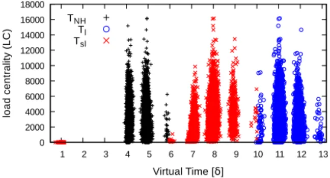
After convergence of NH , our theoretical analysis predicts a time of 2×(D−1) to achieve full load convergence, while simula-tions show that it requires much less than that. This improvement is given by the parallelization of the two processes and can be seen in Fig. 3, which reports all values of TNH, Tsland Tl.
0 2000 4000 6000 8000 10000 12000 14000 16000 18000 1 2 3 4 5 6 7 8 9 10 11 12 13 lo a d c e n tr a lit y ( L C ) Virtual Time [δ] TNH Tl Tsl
Figure 3.TNH, Tsl, andTl for all the nodes, 40 simulations, Erd ˝os graphs with diameter 7.
Fig. 3 reports all the results for all the 40 Erd˝os graphs with diameter 7 (networks with different parameters are not shown as they behave similarly) and shows that at time 6, when the last RT converges, some nodes already reach self convergence. Similarly at time 10, when all nodes reached self convergence, some nodes already reached full convergence. This is because the three processes are concurrent and thus, on typical networks, full convergence time is smaller than in the worst case scenario. Fi-nally, note the small group of nodes which reach self convergence in only one time unit. This is a minimal fraction of leaf nodes produced by the Erd˝os generator whose LC is initially set to zero and never changes.
5
I
NCREMENTALLYD
EPLOYABLEP
ROTOCOL While so far we discussed the theoretical properties of the pro-posed algorithm, in this section and in the following one we focus on how our proposal can be implemented extending a real-world DV routing protocol. To this end we describe its incremental deployment on top of a DV protocol in which two kinds of nodes will coexist: legacy nodes running the legacy version of the protocol and upgraded nodes running the updated version.RFC 6709 of IETF [42] provides general considerations about extension mechanism for networking protocols. A fundamental recommendation to design an extendable and incrementally de-ployable protocol is to employ type-length-value (TLV) packets to define protocol messages. Using TLVs it is easy to enrich a protocol and build a new and backward-compatible version, sim-ply defining new TLVs. This means that upgraded nodes will not violate the syntax and semantics of all legacy protocol messages, but instead they are able to include additional information in them. Legacy nodes are typically designed to store and silently forward the information they are not able to interpret.
Many popular protocols designed for extensions implement this scheme. Three noteworthy examples are OLSR, Babel and BGP that, with its Optional Transitive Attributes, constitutes a prominent example of the so called Silent Propagation Scheme. These three protocols represent all possible routing categories, respectively: LS, DV and path-vector (PV).
In our context, legacy nodes perform only a basic DV routing protocol based on Bellman-Ford: therefore they will silently prop-agate the additional messages that upgraded nodes generate and process to perform the algorithm for LC. To do an incremental de-ployment Algorithm 1 is not suitable, and we need supplementary notation as described in Table 2 to define the behavior of legacy
Table 2
Notation for Legacy and Upgraded nodes
Field Notation Description
Metric m distance ofvfromdaccording to a given metric
Buffer BUF dictionary mapping destinations d to the list of
subTLVs contained in recent advertisements ford
Routing Table RT dictionary mapping destinationsdto distances
ex-pressed in a given metricm
SubTLV stv tuple of information, appended to a parent TLV
such as a Route-Advertisement Forwarded
subTLVs fwd list of subTLVs
Source of loadsource id of the upgraded node generating a contribution
Remote NH rNH next-hop selected by a remote upgraded node toforward its subTLVs
Splitted
Contributions splitC
load contributions that an upgraded-nodevsends toward destination d. Ifv has more NHs for d, contributions are evenly split before begin sent
and upgraded nodes. The logic of a legacy node is represented in Algorithm 2, while an upgraded node extends this logic as shown in Algorithm 3.
As for all DV routing protocols (such as the classical RIP, or Cisco EIGRP, or the Babel protocol adopted later in this work), the Bellman-Ford algorithm is used to maintain a Routing Table (RT ) mapping each destination to a next hop and a distance. An RT is a dictionary mapping destinations d to distances expressed in some given metric m. We use the square brackets operator to retrieve the information regarding a particular destination d recorded in RT , i.e., RT [d] = (m, NH ). We use the dotted notation to access single fields of the tuple, as in RT [d].NH . For a dictionary, the ‘()’ operator returns the list of the keys of the dictionary, i.e., RT () = [d0, d1. . . dN]. The ‘[]’ and ‘{}’ symbols refer to the empty list and dictionary, respectively. Note that NH is an array of next hops, therefore we support routing protocols that implement multipath routing.
A legacy node owns a buffer (BUF ) to store the list of subTLVs that neighbors may attach to route-advertisements. On line 9 of Algorithm 2, a legacy node starts the routine to process a generic advertisement containing a destination d with cost m together with fwd , i.e., a list of subTLVs that the sending neighbor u may have silently forwarded. On lines 10-14, the node performs the classic update of its RT selecting the NH that offers the shortest-path to reach the advertised destination. Multipath is supported by maintaining more next-hops if they offer paths with equal cost (line 14). While processing a received advertisement, a legacy node is not able to parse attached subTLVs, therefore it can only put them all in its buffer as shown in lines 16-18. In particular, subTLVs are indexed by d and marked with the id of the sending neighbor and have a limited time validity. Before storing subTLVs in BUF buffer, the legacy node discards previous information received by the same neighbor for the same destination (line 15).
The silent propagation of subTLVs is implemented when sending route advertisements (line 8), sent periodically when the node sends DVs to all its neighbors1. Beyond the funda-1. It is usually required to send different DVs to different neighbors, think for instance of the classic split-horizon technique widely used to mitigate the well-known count-to-infinity problem.
Alg. 2: Logic of a Legacy node v
1 Init:
2 RT [v].m = 0; RT [v].NH = [ ]; BUF [v] = [ ] 3 Repeat every δ seconds:
4 Cleaning(now ) . Clean expired subTLVs from BUF 5 foreach u, d ∈ neighbors × RT () do
6 if u ∈ RT [d].NH then
7 fwd = BUF [d] . forward subTLV only on SPs 8 send hd, RT [d].m, f wdi to u 9 on receive hd, m, fwd i from u do // Bellman-Ford 10 if d /∈ RT () OR m + C[u] < RT [d].m then 11 RT [d].NH = [u] 12 RT [d].m = m + C[u]
13 else if m + C[u] == RT [d].m then 14 RT [d].NH .append(u)
15 Cleaning(u, d) . Clear old subTLVs from u to d 16 foreach stv ∈ fwd do
17 stv .holdTime = now + ε
18 BUF [d].append(hu, stv i) . Buffer subTLVs
// DictionaryC[·] contains the cost of the links to neighbors
Alg. 3: Logic of an Upgraded node v
1 Init:
2 RT [v].m = 0; RT [v].NH = [ ]; RT [v].loadIn = { } 3 Repeat every δ seconds:
4 Cleaning(now ) . Remove expired contributions 5 foreach u, d ∈ neighbors × RT () do
6 if u ∈ RT [d].NH then
7 loadOut = 1 . Generate/send contrib on SPs 8 foreach u ∈ RT [d].loadIn() do
// Aggregate received contributions
9 loadOut += RT [d].loadIn[u] 10 splitC = loadOut /|RT [d].N H|
// subTLV with sourcev sent via u
11 stv = (v, u, splitC)
12 send hd, RT [d].m, stv i to u
13 on receive hd, m, fwd i from u do // Bellman-Ford as in Algorithm 2, plus // Process list of subTLVs attached tod
14 foreach stv ∈ fwd do 15 source, rNH , C = stv
// Index received contributions by source andrNH
16 RT [d].loadIn[source, rNH ] = splitC
17 RT [d].loadIn[source, rNH ].holdTime = now + ε
/* The load centrality ofv is given summing up all contributions inRT ().loadIn. */
mental advertisement of the destination d with the best known cost RT [d].m, legacy nodes also forward all the subTLVs that were contained in advertisements announcing d. The subTLVs to propagate are retrieved from the buffer (lines 5-7). Due to the control performed on line 6, subTLVs are forwarded only to valid neighbors: assuming routing convergence this means that subTLVs flow through shortest paths only.
parse subTLVs. SubTLVs define what we call centrality contribu-tions, which are the minimal amount of information required to run the distributed protocol for the computation of LC. The logic of an upgraded node is described by Algorithm 3. Fundamentally, an upgraded node is able to generate and send contributions (lines 5-12), and also to aggregate and store the contributions it may receive (lines 14-17): summing up all the received contributions an upgraded nodes determines its own LC index.
When an upgraded one receives a route-advertisement (line 13), it does not ignore the attached subTLVs, but it rather parses them as shown on line 15. Line 15 defines the pieces of informa-tion that compose a centrality contribuinforma-tion, which are:
• source: the id of the remote node (in fact, it may not be a direct neighbor) that generated this contribution;
• rNH : the NH towards which the remote node sent the contribution;
• splitC: the amount of forwarded load, with the same mean-ing of θs,d(v) of Definition 1.
The received contributions are stored in RT indexed by their source but also by their rNH (line 16): rNH is required to distin-guish contributions split remotely by the same source that need to be summed up in aggregation points reached after flowing through different paths. Stored contributions have a limited time validity (line 17). If a node stops being part of a given path, because of a new routing decision by a remote node, after some time this node will properly forget the contribution received previously on that path. Expired contributions are discarded invoking periodically a cleaning routine (line 4).
An upgraded node is able to create subTLVs to send centrality contributions. Similarly to the advertisement sent by legacy nodes, also upgraded nodes customize their announcements for their various neighbors. They offer their unitary load contribution (line 7), and the aggregation of all other contributions directed to the same d (lines 8-9), to those neighbors that lie on the shortest paths towards d. Compared to Algorithm 1, the aggregated load directed to d is equally split among all possible NH before being sent (line 10); finally a subTLV defining a centrality contribution is generated (line 11).
6
P
ERFORMANCE OF THED
ISTRIBUTEDLC C
OM-PUTATION WITH
P
ARTIALI
NFORMATIONConsider a network in which only a subset H ⊆ V of upgraded nodes participate to the protocol, while the legacy nodes in W = V \ H do not participate. A node h ∈ H generates one unit of commodity towards every other node v ∈ V, while a node w ∈ W does not generate any commodity. Every node h also aggregate and split commodity contributions when necessary and, above all, h estimates its own centrality and those of all other nodes in H. Legacy nodes store the contribution field of the update packets they receive in their routing table as opaque metadata, and pass it to the next hop when they generate their own update packets. In this scenario, the upgraded nodes can only compute an underestimate of their LC indexes, and it is interesting to analyze how quickly this estimation reaches the true value increasing the number of updated nodes. We start by proving the following corollary:
Corollary 2. Given a graph G and a set H ⊆ V of nodes that support the protocol, ifG remains stable for a long enough period
of time then, for each nodeh ∈ H, the ‘load ’ variable maintained byh will eventually converge to:
LC0(h) = X s∈H
X
d∈V
θs,d(h) (4) Proof. The proof is straightforward from Theorem 1. When con-sidering a topological sort and a node uk, then from all nodes in {u0. . . uk−1} only those that belong to H generate the load contribution after collecting the messages. The total number of contributions that uk receives for destination d is thus given by |{u0. . . uk−1|ui∈ H}| and loadOut[d] =Ps∈Hθs,d(uk). The same happens for every other destination, which means that with partial deployment, Algorithm 3 computes a partial version of the load centrality corresponding to Eq. (4).
6.1 Error Estimation with Partial Coverage
Corollary 2 is simple but powerful; it shows how, with reasonable assumptions on the legacy nodes, we can exploit LC incrementally and we can estimate the load centrality ranking even with partial information. In the rest of the section, we go one step forward and give a theoretical analysis of the average error introduced in the estimation. An experimental study of how this error impacts the nodes’ ranking in terms of centrality is presented in Sec. 6.2. 6.1.1 Error function definition
Given an arbitrary H, with H = |H|, we state the following: Def. 3:Average Normalized Load Centrality
4 LC = 1 N X v∈V LC(v) = 2 P v∈VLC(v) N2(N − 1) (5) Def. 4:Average Normalized Partial Centrality
4 LC0= 1 H X h∈H LC0(h) = 2 P h∈HLC 0(h) H2(N − 1) (6) Considering a partial deployment (i.e., looking at Eq. (6)), the average is computed only over nodes belonging to H (which are H instead of all N nodes); the normalization coefficient changes accordingly. We are interested in computing the average normalized relative error EHdefined as:
Def. 5:Average Normalized Relative Error
EH= 4 LC − 4 LC0 4 LC (7) We characterize analytically the relative error defined in Eq. (7), rewriting it in terms of two main factors that describe the “missing load contributions", which are lost because only a subset of nodes, namely H ≤ N , perform the algorithm. This reformulation en-ables us to derive lower and upper bounds for EHand understand how it converges to zero for H approaching N . To this purpose, we start computing the expected overall load in the network with the following theorem.
Theorem 2 (Overall Network Load). X
v∈V
LC(v) = N (N − 1)l (8) whereN (N − 1) is the number of (s, d) pairs in V with s 6= d andl is the average shortest path length in V.
s d Hops 1 0.5 0.25 0.25 0.5 1 1 2 3 4 0.5 s d 1 1 1 1
a)
b)
(a) Propagation of a contribution over a single path.
s d Hops 1 0.5 0.25 0.25 0.5 1 1 2 3 4 0.5 s d 1 1 1 1
a)
b)
(b) Splitting of a contribution over multiple paths.
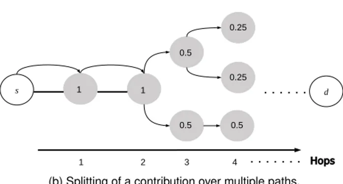
Figure 4. Considering the load contribution derived from the commodity generated bysand sent tod, this contribution transits through all nodes drawn in solid color.
Proof. Consider a shortest path between s and d as a sequence of nodes {s, . . . d} and the path length as (|{s . . . d}| − 1) without loss of generality2.
Consider the generic propagation of a commodity unit from node s to node d on a single shortest path as depicted in case Fig. 4a. All the nodes that forward the commodity increment their load centrality metric by the amount of commodity they have forwarded, which is 1. This means that the commodity sent by source s to target d, by traveling on the shortest path from s to d, induces an overall increment of load in the network equal to the length of the shortest path linking s to d (|s . . . d| − 1).
If there are multiple shortest paths, as in case of Fig. 4b, we assign load 1 to s itself (distance 0). At some distance i > 0 from s the path splits in k equivalent paths, then there are k nodes at distance i + 1 from s, and by definition the sum of the load centrality of nodes at distance k + 1 equals the sum of load centrality at distance k. By induction, given the load at distance 0 equal to 1, the sum of the load of the nodes at any distance k + 1 is 1 and the total load induced on the network equals (|s . . . d| − 1). Extending this observation to all the N (N − 1) possible (s, d) couples the overall load in the network is equal to the sum of the lengths of all the shortest paths, which by definition is N (N − 1)¯l.
Combining Eq. (8) and Eq. (5), we can rewrite the Average Normalized Load Centrality as:
4 LC = 2l
N (9)
We now need to reformulate the termPh∈HLC0(h) in the right hand side of Eq. (6) adopting an approach similar to the one used to prove Theorem 2. In the partial deployment scenario, only shortest paths linking nodes h ∈ H to destinations in v ∈ V are accounted for to estimate the load due to the commodity propagation; consequently, the average path length l used in Theorem 2 should be computed on the proper subset of shortest paths that are actually used. We call l0 the average path length 2. If there are multiple minimum shortest paths for some endpointssand
d, then they all have the same path length. Forsdirectly connected todthe path length is 0. The distance definition implies that we exclude from the computation of LC for nodevthe contributions of paths terminating inv.
from all sources h ∈ H to destinations in v ∈ V. Furthermore, we measure the centrality for the subset of nodes in H, which are the only ones implementing the algorithm, based only on the commodity they generate. This means we need to discard all contributions that transit through legacy nodes in W if we want to sum up only the load centrality computed by nodes in the H set. Taking into account these two considerations we define the Overall Estimated Load as follows:
Def. 6:Overall Estimated Load X
h∈H
LC0(h) = H(N − 1)l0− X w∈W
LC0(w) (10)
We can now rewrite the definition of Average Normalized Partial Centrality applying Eq. (10) to Eq. (6):
4 LC0= 2H(N − 1)l 0−P w∈WLC 0(h) H2(N − 1) (11) and this leads to the main reformulation of the Normalized Relative Error EH: EH= 1 − N l l0 H |{z} E1 − P w∈W LC0(w) H2(N − 1) | {z } E2 (12)
where E1and E2are the two factors accounting for legacy nodes missing commodity.
6.1.2 Error function analysis
To gain insight into Eq. (12) we need to understand the roles of E1and E2. Based on the definition from Eq. (10) we observe that E1 describes the load produced by commodity generated by the upgraded nodes, while E2describes the amount of commodity that can not be measured (must be subtracted) because legacy nodes do not accumulate it as they do not understand its meaning.
We start the analysis setting E2 = 0, which yields the error function in Eq. (13) and corresponds to a system where legacy nodes do not generate commodity and were chosen among the nodes that have zero centrality.
EH= 1 − N H
l0
l (13)
This is a relevant case because it is equivalent to the estimation of betweenness centrality using only a restricted number of single-source shortest-paths computations from a set of selected pivots [20]. This approach can be used with a centralized algorithm when the number of nodes is too large to compute all possible shortest paths. Assuming pivots are chosen at random, then l0 quickly converges to l and the error is dominated by N/H. There are many works in the literature that deal with this problem, given that the execution of superlinear algorithms can be unfeasible when the graph is in the order of billions of nodes (see the work of Riondato et al. and cited bibliography [25]). Our problem is different because we run a distributed protocol, with legacy nodes not generating any load and not even estimating their centrality. This is why, in Eq. (10), we subtracted contributions traversing nodes in W, and hence E2≥ 0.
Let us now go back to consider the original scenario in which we have a non-negligible number of legacy nodes that are not able
to estimate their centrality. How big can E2 be? Consider these two extreme cases:
1) W includes all and only the nodes with zero centrality; 2) W includes all and only the nodes with non zero centrality.
In the first case P
w∈WLC0(w) = 0 and we fall back to Eq. (13). In the second case, the sum of the centrality of all nodes in W accounts for the overall load generated in the network, which is: H(N − 1)l0. Then E
1 = E2 and the relative error is 1: Essentially we are trying to estimate the centrality of nodes in H which do not lie on any shortest path. No matter how many shortest paths we consider, the relative average error will be always 1. Consider for instance a star graph: for any size of H, if H does not include the star center then the relative error will always be 1.
In between these extremes, we note that, from Eq. (10): l0= P h∈HLC 0(h) +P w∈WLC 0(w) H(N − 1) = P v∈VLC 0(v) H(N − 1) (14) then we have: E1= l0 H = P v∈V LC0(v) H2(N − 1) ≥ E2 (15) which means that EH always lies in between the two extreme cases we just described, but also that upgrading more central nodes the error done is smaller.
Summing up, the convergence of the relative normalized error is quite slow. In the best case where E2' 0, then EH ' 1 −NH, meaning that with 80% nodes coverage we underestimate with a 25% error. Anyhow, the average error does not say much on how the ranking is influenced and, in general, centrality rankings are more important than the single centrality values. Estimating the error on rankings is less straightforward than the average error, but crucial. In Sec. 6.2 we compute rank correlation coefficients and show that, even for very small fractions of upgraded nodes, the algorithm preserves correct ranking with great accuracy.
6.2 Centrality Ranking with Partial Information
We implemented the new distributed, incrementally-deployable algorithm in a Python simulator. We used this simulator to study the Spearman’s rank correlation coefficient rs[43] and so evaluate the degree of similarity between rankings computed respectively with the exact and the approximated algorithms we provided (i.e., with Algorithm 1 and Algorithm 3). Spearman’s rsmeasures the correlations of two rankings of the same population, and ranges in [−1, 1]. When rs = 1 the two rankings are perfectly correlated, when rs = −1 one ranking is perfectly specular to the other, when rs= 0 there is no correlation between the two rankings.
We analyzed graphs generated using four well known gen-erators: the already cited Barabási-Albert and Erd˝os plus the Waxman [44] and Caveman [45] models. As in the previous experiments, we generate 10 graphs of various size for each diameter (from 3 to 7, for a total of 50 graphs). The results shown in Fig. 5 are obtained following this methodology:
• For each graph we compute the exact centrality ranking using the algorithm with H = V;
• For each graph we also choose 5 instances of H at random, with H size ranging from 10% to 100% of V size, and we run a simulation. Each run produces an estimated ranking for the elements of H. 0.7 0.8 0.9 1 10 20 30 40 50 60 70 80 90 100
Spearman Rank Correlation r
s
Upgraded nodes penetration ratio [%] ER BA CV WX
Figure 5. Spearman’s rs for Barabási-Albert, Erd ˝os, Waxman, and Caveman graphs for 1000 nodes and diameter 5 with 95% confidence intervals.
• Finally, for each run we compute Spearman’s coefficient comparing the estimated and the exact rankings (limited to the nodes in H), and we average it on the 50 runs for that diameter (10 graphs times 5 random choices of H).
For brevity, we report here only the results with 1000 nodes and diameter 5, but we obtained results with similar trends also for all the other diameter values and with graphs of 400 nodes.
Fig. 5 reports the Spearman’s correlation coefficient between the exact ranking and the estimated ranking, on the 4 families of graphs. It shows that for any kind of graph, with H covering 30% of V, the correlation rs is already close to 0.8, while with a coverage of 60% the correlation goes over 0.9 for all graphs. Fig. 5 confirms that estimated ranking accurately classifies nodes for their importance; they can therefore be used to fine-tune network protocols even in presence of a small fraction of updated nodes.
7
T
UNINGB
ABEL WITHC
ENTRALITYOut of the many contexts in which our algorithm can be exploited, we focus on advantages it can give to optimize DV routing protocols in wireless mesh networks. To perform link sensing in wireless networks, routing protocols define a timer tHused by each
node to control the generation of link-level HELLO messages. This timer is crucial for a fast re-convergence in case of failures. A trade-off must be found between a short timer, which guarantees fast detection of link failures but subtracts link capacity to data traffic, and a long timer, that is more resource-aware but makes route convergence slow.
Maccari and Lo Cigno have introduced an optimization of tH based on betweenness centrality [4]. Initially, they define the
average overhead per link (OH) when every node is configured with the same tH. Then, they introduce a loss metric to express the
average estimated loss due to a node failure:
L(k) = VHtH(k) N (N − 1)bk (16) where VHis a protocol parameter (the number of consecutive lost
packets after which a link is considered broken). Finally they show that keeping OHconstant, the average loss can be minimized if tH
is configured per-node as follows: tH(i) = √ di √ bi tH PN j=1pbjdj PN j=1dj ∝ √ di √ bi (17)
where bi and di are the betweenness and degree of node i. In practice, if a node knows diand bifor all nodes, it can auto-tune its tH(i) to achieve a convergence time distribution that minimizes the
average network disruption after a node failure, keeping a constant signaling overhead in the network.
The authors used this technique for the OLSR protocol but, in principle, it can be applied to any link-state protocol where every node is aware of the whole topology. Conversely, it cannot be applied to DV routing protocols because, in this latter case, nodes have a limited topological knowledge and cannot compute Eq. (17). Algorithm 1 does not mandate nodes to know the entire topology and it is fully distributed, therefore its implementation on a DV routing protocol is straightforward and we effectively integrated it with the Babel protocol [15], a well-known DV routing protocol3.
We implemented the distributed centrality computation algo-rithm in babeld, the open source implementation of Babel, in order to verify that centrality can be correctly computed. The evaluation strategy and performance metrics are those proposed by the authors of [4]; here, we just briefly recall them, while a detailed description is provided in the original paper. Finally, note that to use Eq. (17), the propagated distance vector should also contain the degree of node i. If we drop this requirement, then we can set tH(i) =
√ ti √
biK for some constant K. This will still optimize
the timers and keep a constant level of global overhead, but it will not produce exactly the same overhead OH of the default configuration. In return, it greatly simplifies the protocol as long as every node can take decisions based only on its own centrality. For our purpose, we used the value of K that generates the value of OH corresponding to tH= 1s.
We run the code in an emulated network using the Mininet platform. At time tf, we trigger the failure of node k, and we let all routing tables stabilize again; we repeat this procedure for a subset of Nf ≤ N nodes. Note that generally Nf < N because we exclude two categories of nodes: leaf nodes (their centrality is zero so their failure does not impact any other node) and cut-points (nodes whose centrality may be high but they partition the graph in disconnected components, so that it is not possible to route around the failed node). During experiments we dump the routing tables RTji[d] every 0.5 s: a dump contains the matching between a destination d and the next hop nh for node i at time tj (only one path is used in Babel). When the emulation is over, we group the dumped routing tables according to timestamps, next we recursively navigate each group to take a snapshot of all shortest paths from every source s to any destination d. We call Lj the number of broken shortest paths that, for tj > tf, are incomplete or still pass through node k and we define Lbabel(k) =PjLjthe total loss value when the emulation runs with the original babeld and Lcent(k) the same value but computed using the optimized timers. Finally we compare the two approaches, computing the relative loss value averaged over all possible failures as:
L = 1 − PNf k=0Lcent(k) PNf k=0Lbabel(k) (18)
3. Eq. (17) uses betweenness centrality, while our approach computes load centrality. However, in a mesh network links are weighted by their quality (with any metric the protocol supports), which makes it hard to have multiple paths with the same exact weights, therefore, in real-world mesh networks load centrality converges to betweenness centrality. This said, we do not attempt any comparison with [4]: comparing a DV and a link-state protocol goes well beyond comparing centrality metrics.
If L > 0, then the tuned version of babeld, averaged over Nf failures, produces lower loss compared to the non-modified version, always keeping the same overhead due to control messages.
Before presenting detailed results, it is worthwhile to discuss some modifications to Algorithm 1 that are necessary to imple-ment it in babeld and are in general required for any real DV protocol.
Nodes vs. Routers. The common approach it the literature focused on centrality is to treat nodes as sources, targets and forwarders of traffic. In real networks, sources and targets are IP addresses and routers have several interfaces with distinct IP addresses. To overcome this issue, we aggregate all route-updates coming from the same node based on the “router-id” field defined by Babel to uniquely identify a router. This field is included in all packets generated by a router and is propagated by all others, therefore we can aggregate the centrality contributions pertaining to different interfaces of the same router and do a mapping between IP addresses and graph nodes.
Load Estimation. In our implementation, every router gener-ates a unit of traffic θs,d = 1, but in real networks this value can be arbitrarily tuned. It can be proportional to the dimension of attached subnets (assuming more IPs will generate more traffic) or it can be replaced with an estimation of the real outgoing traffic measured locally. This way load centrality would effectively represent the expected load on the node.
Protocol-specific Heuristics. In our tests we used networks that have more than one shortest path with the same weight connecting the same endpoints (s, d). The version of Babel that we used does not support multipath routing: in these cases Babel performs a tie-break to select one path over another. We also noticed that babeld sometimes selects paths that are not minimum weight. This is probably due to an implemented heuristic that prevents changing from one path to another if their weight is similar, just to avoid route flapping. Our algorithm follows choices taken by babeld, which is the correct behavior on-line even if the computed LC minimally diverges from the theoretical one. Sec. 7.1 further details and explains this issue.
7.1 Experimental Results with Full Coverage
We test the protocol on several topologies extracted from real-world networks [46]. Two of them are Ninux and FFGraz4 the same ones used and published by the authors of [4], which are topologies of two large-scale wireless mesh networks. We were able to collect two more real network topologies, namely Auerbachand Adorf, analysing information provided by the Frei-Funk German community network (CN). FreiFrei-Funk is an umbrella name that gathers together hundreds of wireless CNs in Germany: some of them are made of few nodes, some others are made of hundreds, all of them are mesh networks used to offer Wi-Fi connectivity. Information on these network topologies is freely available (with some effort to understand the format) from the community website5. In the particular case of Auerbach and Adorf,
these two are heterogeneous networks, with a mix of wireless and wired links inside a single routing domain. Finally, we also use 4 others extracted from the well-known Topology Zoo [47], namely Interoute, Ion, GtsCeand TataNld; these are 4 wired topologies of
4. https://www.ninux.org — https://graz.funkfeuer.at/en/about.html 5. See https://api.freifunk.net, and the visualizer https://www.freifunk-karte. de.
0 1000 2000 3000 4000 5000 6000 0 20 40 60 80 100 120 140 lo a d c e n tr a lit y ( L C )
Nodes sorted by loadoffline
LCoffline
LCbabel
Figure 6. Comparison of LC computed on-line with and off-line with networkx on the same topology computed by Babel
0 2000 4000 6000 8000 10000 12000 14000 16000 0 10 20 30 40 50 60 70 # B ro k e n P a th s ( Lj ) Time [sec] cent babel
Figure 7. Comparison of the network loss in ninux topology after the failure of one of the most central nodes
similar size that we use to extend our analysis. Table 3, discussed later on, reports the names of all the 8 topologies with their key characteristics and the loss reduction.
Babel is an event-driven protocol where messages are sent in reaction to detected changes and expiration of local timers. This, together with the heuristics mentioned in the previous section, introduces slight differences in the centrality computation compared to the ideal protocol presented in Sec. 3. Fig. 6 presents a validation of our implementation in babeld and reports a comparison between empirical and theoretical LC values com-puted for all nodes in a network. On the one hand, LC has been computed on-line using the modified babeld and, on the other hand, running Python networkx libraries off-line on the same topology built by babeld and saved in JSON format. The Mininet network emulator allows running experiments with real instances of babeld over real-world networks6. For instance, the results
shown in Fig. 6 are obtained running experiments on the topology of ninux, a CN of Rome.
First of all we verified that the sum of all LC values is identical in both cases, which means that Babel never uses a minimum weight path that is longer (in terms of hops) than the shortest one computed by networkx. Next, we noticed that nodes’ rankings are not exactly the same, but very similar.
Fig. 7 reports the number of broken paths vs. time after one of the most central nodes of the ninux topology has failed around time t = 5 s. A path is said to be broken if it contains a node with an invalid next-hop. Babel with centrality reacts slightly faster, but above all recovers more routes in less time compared to standard Babel. Thus we achieve a resilience gain without adding any cost, 6. Experiments cannot be run directly on working networks to avoid disrupting their daily functioning.
as the complexity of LC computation is minimal: in fact, the signaling overhead in terms of number of messages is constant, while messages’ dimension increases only marginally.
Table 3
Loss reductions in real networks
Network |V| |E| Nf Loss Reduction Type
Interoute 110 148 63 8.37% Wired Ion 125 146 58 3.10% Wired GtsCe 149 193 98 6.05% Wired TataNld 145 186 68 7.34% Wired Ninux 126 147 17 10.65% Wireless FFGraz 141 200 19 13.11% Wireless Auerbach 123 223 70 11.29% Heterogeneous Adorf 123 225 65 13.27% Heterogeneous
To get exhaustive results, we run the modified version of babeld over a total of 8 emulated networks representing real topologies. Table 3 and Fig. 8 report the results summary. Fig. 8 compares Lbabel(k) and Lcent(k) where nodes k = 1, 2, . . . , 15 are the 15 most central ones for each topology. The chosen networks are ninux (Fig. 8a), Graz (Fig. 8b), and Ion (Fig. 8c), because they represent well different classes of networks; however results would not change significantly selecting other networks. As we can see, in general Lcent is smaller than Lbabel, but sometimes the fine-tuned timers’ frequency does not provide any gain. However, a closer look to Table 3, which reports the mean loss reduction for all the 8 considered networks, reveals that averaging over all possible failures we obtain a global gain, ranging from 3% up to 13% depending on the topology; still it is always a clear advantage in favor of tuning timers based on centrality.
In general, wireless and heterogeneous networks achieve larger gains compared to wired and uniform networks due to structural properties of the network graphs. In fact, the optimization level that can be achieved exploiting centrality strongly depends on the array of values of bi and di and on the availability of alternative paths to route around a failure. Consider the extreme case of a ring network, or in general an n-regular network over a torus: in such networks all nodes have same degree and centrality and Eq. (17) returns the same value for all timers. In these cases no optimization is possible.
7.2 Analytical Results with partial Coverage
We conclude this section showing we can obtain a performance improvement even when only a subset of nodes support centrality-based optimization, applying the algorithms explained in Sec. 6. We use the Python simulator introduced in Sec. 6.2 with the fol-lowing procedure. Given a network with N nodes and ρ ∈ (0, 1], we randomly select dρN e nodes that run Algorithm 3, while all the other nodes run Algorithm 2. We let the network converge and we obtain the estimated values of centrality bk for the upgraded nodes. Then we compute the average loss exactly as explained in Sec. 7, but, instead of running full emulations, for performance reasons we compute Lbabel and Lcentin Eq. (18) using Eq. (16). The different methodology makes the analytical value of L differ-ent from the data we obtain with emulations. These results must be considered as an upper bound of the possible improvement, and thus Fig. 9 is not directly comparable with Table 3. On the other hand, this allows repeating the process for 40 times, for ten values of ρ and for all the networks in Table 3 in reasonable time.
0 50 k 100 k 150 k 200 k 250 k T otal Loss
Failed node sorted by LC
Lcent Lbabel (a) Ninux. 0 50 k 100 k 150 k 200 k 250 k 300 k 350 k 400 k T otal Loss
Failed node sorted by LC
Lcent Lbabel (b) Graz. 250 k 300 k 350 k 400 k 450 k 500 k 550 k 600 k 650 k T otal Loss
Failed node sorted by LC
Lcent
Lbabel
(c) Ion.
Figure 8. Comparison of the loss induced by the failure of the 15 more central nodes in ninux (a) Graz (b) and Ion (c) when standard Babel is used (Lbabel) or the modified version is used (Lcent)
-10 0 10 20 30 0.1 0.2 0.3 0.4 0.5 0.6 0.7 0.8 0.9 1 Loss Reduction [%] ρ FFGraz Interoute Auerbach GtsCe Ion Ninux TataNld Adorf
Figure 9. Comparison of loss on various networks with only a fraction
ρof nodes supporting the improved protocol. For clarity, we report the 95% confidence interval for Adorf only, which has the largest ones in average. The intervals are barely visible.
Fig. 9 shows that with ρ larger than 0.2, in all networks we
start to have a tangible improvement compared to the standard behavior. This confirms that even if the convergence to the exact centrality values is slow, it it sufficiently precise to improve the protocol performance with as little as 20% of the upgraded nodes. Such a result is very encouraging as it finally shows that we can deploy centrality-based optimizations in an incremental way on existing networks, and obtain a net improvement way before the full coverage is reached. This is a key step in the path to improve protocols in large-scale existing networks.
The fact that some of the curves are not monotonically growing is probably a combination of several effects. First, when we apply the improved protocol to a subset of nodes, we cannot strictly enforce the condition of constant average overhead OH. We expect this condition to hold in average as ρ approaches 1. Second, due to the specific properties of each topology the convergence of the centrality estimation may be faster or slower, and could even suffer from a bias. As a result it could be that in Ninux and FFGraz for some choices of ρ we slightly overestimate centrality, and thus we produce a higher gain than with larger values of ρ.
8
C
ONCLUSIONSCentrality metrics are key for understanding the importance of a node in a network, and they have been extensively used in many scientific fields. Betweenness and load centrality are two of the most popular ones. In networks that do not support multipath routing the two metrics coincide, and this is the case for most communication networks.
In spite of its importance, and before this work, there was no fully distributed algorithm that supports the computation of load centrality in generic networks. In fact, among existing algorithms there are those requiring a full topological knowledge, those that are distributed but only approximated, and those that are exact and distributed but applicable only on special topologies (such as DAGs or trees). For this reason so far it was impossible to exploit betweenness or load centrality in distributed network protocols.
This paper contributes, to the best of our knowledge, the first algorithm for the exact computation of load centrality in a generic graph. We demonstrated its convergence, the worst case convergence time, and we showed it can be directly integrated with minimal modification into a distance-vector (DV) routing protocol. We provided a direct use-case implementing the dis-tributed algorithm in Babel, a widely used standard DV protocol, showing it can tangibly improve the convergence time in case of nodes’ failure for all tested topologies, taken from real networks.
Finally, the algorithm does not require all nodes in the network to support it; it can be gradually deployed in an existing network and even with a small fraction of upgraded nodes it yields useful rankings for node centrality. Many more applications than routing can benefit from nodes’ rankings based on centrality. Caching is the most obvious, but not the only one. We believe that the availability of efficient centrality computation algorithms can spawn research and applications exploiting it.
R
EFERENCES[1] L. Maccari, L. Ghiro, A. Guerrieri, A. Montresor, and R. Lo Cigno, “On the Distributed Computation of Load Centrality and Its Application to DV Routing,” in IEEE Int. Conf. on Computer Communications (INFOCOM), Honolulu, HI, USA, Apr. 2018, pp. 2582–2590. [2] U. Brandes, “On Variants of Shortest-Path Betweenness Centrality and
their Generic Computation,” Social Networks, vol. 30, no. 2, pp. 136– 145, May 2008.