Space time adaptive processing in multichannel passive radar

(1)

UNIVERSITÀ DI PISA

Scuola di dottorato in Ingegneria “Leonardo da Vinci”

Corso di Dottorato di Ricerca in

TELERILEVAMENTO

Tesi di Dottorato di Ricerca

“Space time adaptive processing in multichannel passive radar”

Autore

Relatori

Christian Moscardini

__________________

Prof. Fabrizio Berizzi

___________________

Prof. Marco Martorella

____________________

(2)

Abstract

Nowdays, passive bistatic radar (PBR) systems have become a subject of intensive research, owing essentially to its unique features, such as low probability of interception, small size and low cost. Passive radar is a concept where illuminators of opportunity are used. In a bistatic passive radar the main challenges are: estimating the reference signal which is required for detection, mitigating the direct signal, multipath and clutter echoes on the surveillance channel and finally achieving a sufficient SINR to detect targets.

This thesis is concerned with the definition and application of adaptive signal processing techniques to a multichannel passive radar receiver. Adaptive signal processing techniques are well known for active pulse radars. A PBR system operates in a continuous mode, therefore the received signal is not avalaible in the classical array elements-slow time-range domain such as in active pulse radar. A major component of this research focuses on demonstrating the applicability of traditional adaptive algorithms, developed in the active radar contest, with passive radar.

Firstly a new detailed formulation of the sub optimum “batches algorithm”, used to evaluate the cross correlation function, is proposed. Then innovative 1D temporal adaptive processing techniques are defined extending the matched filter concept to an adaptive matched filter formulation. Afterwards a new spatial adaptive technique, based on the application of the adaptive digital beamforming after the matched filter, is investigated. Finally both 1D spatial and temporal adaptive techniques are extended to 2D space-time adaptive processing techniques. Specifically we demonstrate the applicability of STAP processing to a passive bistatic radar and we show how the classical STAP algorithms, developed for active radar systems, can be applied to a PBR system. The new defined passive radar signal processing architectures are compared with the standard approaches and the effectiveness of the proposed techniques is demonstrated considering both simulated and real data.

(3)

List of Figures

FIGURE1.1 PULSE RADAR ARCHITECTURE... 21

FIGURE1.2 CPIDATACUBE... 23

FIGURE2.1 BLOCK DIAGRAM OF THEPBRMATCHED FILTER... 29

FIGURE2.2 SINGLE TARGET SCENARIO... 31

FIGURE2.3 MULTI TARGET SCENARIO... 34

FIGURE2.4 MULTIPATH MODEL... 38

FIGURE2.5 TYPICALPBRSIGNAL PROCESSING CHAIN... 40

FIGURE3.1 CROSS CORRELATION FUNCTION IN THE FREQUENCY DOMAIN... 49

FIGURE3.2 CROSS CORRELATION FUNCTION IN THE TIME DOMAIN... 51

FIGURE3.3 BATCHES ALGORITHM DESCRIPTION... 54

FIGURE3.4 BATCHES ALGORITHM:REFERENCE AND SURVEILLANCE SIGNALS SEGMENTATION... 55

FIGURE3.5 BATCHES ALGORITHM SCHEME... 57

FIGURE3.6 BATCHES ALGORITHMS LOSSES... 59

FIGURE3.7 TRADITIONAL BATCHES ALGORITHM:REFERENCE AND SURVEILLANCE SIGNAL SEGMENTATION... 60

FIGURE3.8 BATCHES ALGORITHM:COMPUTATIONAL LOAD... 61

FIGURE3.9 TIME PROCESSING ELAPSED FOR BATCHES ALGORITHM AND DIRECT-FFTAPPROACH... 62

FIGURE3.10 DVB-TSPECTRUM... 64

FIGURE3.11 GUARD INTERVAL CONCEPT... 65

FIGURE3.12: OFDMMATCHED FILTER:REFERENCE AND SURVEILLANCE SIGNALS SEGMENTATION... 67

FIGURE3.13: OFDMMATCHED FILTER ARCHITECTURE... 69

FIGURE3.14: MODIFIEDOFDMMATCHED FILTER ARCHITECTURE... 71

FIGURE4.1 TEMPORAL ADAPTIVE PROCESSING:TRADITIONAL ARCHITECTURE... 75

FIGURE4.2 ADAPTIVE NOISE CANCELLER STRUCTURE... 76

FIGURE4.3 TEMPORAL ADAPTIVE PROCESSING:ADAPTIVE MATCHED FILTER... 78

FIGURE4.4 TEMPORAL ADAPTIVE PROCESSING:ADAPTIVE MATCHED FILTER PLUS ADAPTIVE NOISE CANCELLER... 79

FIGURE4.5 TRAINING DATA SET SELECTION WITH DIRECTFFTAPPROACH. ... 82

FIGURE4.6 TRAINING DATA SET SELECTION WITH BATCHES ALGORITHM APPROACH... 84

FIGURE4.7 RANGE-DOPPLER MAP BEFORE FILTERING... 88

FIGURE4.8 RANGE-DOPPLER MAP AFTERECAFILTER... 89

FIGURE4.9 RANGE-DOPPLER MAP AFTER OPTIMUM TEMPORAL ADAPTIVE PROCESSING... 89

(7)

FIGURE4.11 EXPERIMENT SCENARIO GEOMETRY[CAPRIA2010]. ... 90

FIGURE4.12 RANGE-DOPPLER MAP BEFORE FILTERING... 91

FIGURE4.13 RANGE-DOPPLER MAP AFTER FILTERING... 92

FIGURE5.1 MULTI CHANNEL SIGNAL MODELLING... 97

FIGURE5.2 DIGITAL BEAMFORMING INPBRSYSTEMS... 99

FIGURE5.3 DATA TRAINING SELECTION... 102

FIGURE5.4 TRADITIONAL ARCHITECTURE... 103

FIGURE5.5 ADVANCED ARCHITECTURE... 106

FIGURE5.6 TRAINING DATA SET SELECTION... 107

FIGURE5.7 ANALOG BEAMFORMING ARCHITECTURE... 109

FIGURE5.8 RANGE-DOPPLER MAP BEFORE SPATIAL ADAPTIVE PROCESSING... 110

FIGURE5.9 RANGE-DOPPLER MAP CONSIDERING ONLY TARGET COMPONENTS... 111

FIGURE5.10 RANGE-DOPPLER MAP AFTER SPATIAL ADAPTIVE PROCESSING RELATIVE TO THE FIRST TARGET... 111

FIGURE5.11 RANGE-DOPPLER MAP AFTER SPATIAL ADAPTIVE PROCESSING RELATIVE TO THE SECOND TARGET... 112

FIGURE5.12 SIMULATED SCENARIO... 112

FIGURE5.13 UNIFORMCIRCULARARRAY WITH PATTERN CARDIOD ELEMENTS... 114

FIGURE5.14 SIMULATED GROUND CLUTTER AND MULTIPATH DIRECTIONS... 115

FIGURE5.15 SINRBEFORE SPATIAL ADAPTIVE PROCESSING... 116

FIGURE5.16 RANGEDOPPLER MAP RELATIVE TO ARRAY ELEMENT1... 116

FIGURE5.17 RANGEDOPPLER MAP AFTER FILTERING... 117

FIGURE5.18 SINRAFTER SPATIAL ADAPTIVE PROCESSING... 118

FIGURE6.1 STAPPROCESSING IN ACTIVE PULSE RADARS... 122

FIGURE6.2 ARRAY PASSIVE RADAR SYSTEM... 124

FIGURE6.3 ARRAY PASSIVE RADAR SYSTEM WITH DIRECTFFTAPPROACH... 126

FIGURE6.4 PBR-DIRECT-FFT-STAPARCHITECTURE... 127

FIGURE6.5 ARRAY PASSIVE RADAR SYSTEM WITH BATCHES APPROACH... 129

FIGURE6.6 PBR-BATCHES-STAPARCHITECTURE... 130

FIGURE6.7 PBR -OFDM-STAPARCHITECTURE... 131

FIGURE6.8 PBRSIMULATION GEOMETRY... 134

FIGURE6.9 RANGE-DOPPLER MAP BEFORESTAP... 135

(8)

Acronyms

AF Ambiguity Function

ADC Analog to Digital Converter

CAF Cross Ambiguity Function

2D-CCF Two Dimensional Cross Correlation

Function

CFAR Constant Fals Alarm Rate

CIP Coherent Processing Interval

DAB Digital Audio Broadcasting

DFT Discrete Fourier Transform

DOA Direction of Arrival

DPI Direct Path Interference

DVB-T Digital Video Broadcasting Terrestrial

ECA Extensive Cancellation Algorithm

FMCW Frequency Modulated Continuous Wave

FFT Fast Fourier Transform

GMTI Ground Moving Target Indicator

ICM Internal Clutter Motion

IDFT Inverse Discrete Fourier Transform

IO Illuminator of Opportunity

LCMV Linearly Constrained Minimum Variance

LMS Least Mean Square

LS Least Square

LSL Least Square Lattice

LSMI Loaded Sample Matrix Inverse

MVDR Minimum Variance Distorsionless

Response

(9)

OFDM Orthoganal frequency Division Multiplexing

PBR Passive Bistatic Radar

PCL Passive Coherent Location

PR Passive Radar

PRI Pulse Repetition Interval

RLS Recursive Least Square

SCA Sequential Cancellation Algorithm

SCM Sample Covariance Matrix

SDR Signal to Direct signal Ratio

SF Stepped Frequency

SFN Single frequency Network

SINR Signal to Noise plus Interference Ratio

SLL Side Lobe level

SMI Sample Matrix Inverse

SRP Synthetic Range Profile

(10)

Chapter 1. Introduction

1.1 Passive radar systems

In recent years there has been a growing interest in Passive Bistatic Radar (PBR) using existing transmitters as illuminators of opportunity to perform target detection, localization and tracking [Kuschel 2010], [Howland 2005]. Bistatic radar may be defined as a radar in which the transmitter and receiver are at separate locations. The very first radars were bistatic, until pulsed waveforms and T/R switches were developed [Kuschel 2010]. Bistatic radars can operate with their own dedicated transmitters, which are specially designed for bistatic operation, or with transmitters of opportunity, which are designed for other purposes but found suitable for bistatic operation. When the transmitter of opportunity is from a non-radar transmission, such as broadcast, communications or radio-navigation signal, the bistatic radar has been called: Passive

Radar (PR), Passive Coherent Location (PCL). In this thesis we use the term Passive Bistatic Radar (PBR) to indicate a passive bistatic radar system.

PBR systems have some significant attractions, in addition to those common to all bistatic radars. There has been considerable work on the theory behind PBR and much has been written about its potential [Baker 2005], [Griffiths 2005],

As well as being completely passive and hence potentially undetectable, they can allow the use of parts of the RF spectrum (VHF and UHF) that are not usually available for radar operation, and which may offer a counter-stealth advantage, since stealth treatments designed for microwave radar frequencies may be less effective at VHF and UHF. Broadcast transmissions at these frequencies can have substantial transmit powers and the transmitters are usually sited to give excellent coverage.

(11)

There are a great variety of signals that can be used for PBR purposes. Their performance in PBR systems will vary significantly, depending on a variety of factors: (i) power density at target (ii) coverage (both spatial and temporal), and (iii) ambiguity function shape depending both on the waveform and on the transmitter-target-receiver geometry. In particular broadcast transmitter represent some of the most attractive choices for long range surveillance application due to their excellent coverage. The most common signals used for PBR applications are FM radio and UHF television broadcasts ([Howland 2005], [Griffiths 2005], [Griffiths 1986], [Howland 1999]), as well as digital transmission such as Digital Audio Broadcasting (DAB) ([Coleman 2008], [Guner 2003]) and Digital Video Broadcasting-Terrestrial (DVB-T) ([Berger 2010], [Bongioanni 2009], [Gao 2006], [Glende 2007], [Langellotti 2010], [Poullin 2005-2010], [Kuschel 2008], [Saini 2005], [Yardley 2007]).

For analogue modulation formats, the ambiguity performance depends strongly on instantaneous modulation. Periodic modulation features, such as the sync parts of the waveform in analogue television waveforms, result in ambiguities. For VHF FM radio the ambiguity performance varies significantly, and some types of music; those with high spectral content) are better than others. For digital modulation formats, the ambiguity performance is much more constant with time, and does not depend on the programme content, since signals are more noise-like. Such signals exhibit a radar ambiguity function that has almost ideal thumb tack nature with excellent range resolution. Digital transmissions are therefore to be preferred, even though they tend to be of lower power than their analogue counterparts. A PBR receiver requires at least two signals in order to perform the matched filter receiver: a copy of the transmitted signal and the received signal from the surveillance area. Therefore the simpler PCL radar system requires two antennas: the first antenna, often called the reference antenna, is used to capture the reference signal and should point in the direction of the transmitter, the second antenna, usually called the surveillance antenna, is used to capture the signals of potential target. If an antenna array rather than single receiver antennas is used then the performance of the passive radar system may be improved. In a bistatic passive radar the main challenges are: estimating the reference signal which is required for detection, mitigating the direct signal, multipath and clutter echoes on the

(12)

targets. The transmitted waveforms is not under control of the radar designer and the sidelobes of the ambiguity function can mask possible target echoes. Different techniques have been proposed to resolve these problems and they can be summarized as [Griffiths 2007]:

Spatial cancellation

Spectral/temporal cancellation

To add additional complexity, if the environment is non-stationary adaptive control of the processing is required. Adaptive signal processing techniques have been studied and developed extensively over several decades, both for radio communications and for radar applications, especially considering active pulse radar.

In this thesis we will demonstrate the applicability of classical adaptive algorithms considering a multichannel passive radar. Alternative passive radar signal processing architectures will be proposed and compared with classical and standard approaches.

1.2 Theoretical background

In this section, the main theoretical notions that will be used during the development of this thesis are described. Section 1.2.1 deals with the definition of the classical monostatic ambiguity function and the main differences with respect to a bistatic geometry are detailed. In section 1.2.2 the theoretical background of the adaptive signal processing techniques is analyzed. Finally in section 1.2.3 the main aspects of the adaptive signal processing techniques defined in the well known contest of active pulse radar are detailed.

1.2.1 Monostatic-Bistatic ambiguity function

The ambiguity function is conventionally derived assuming a monostatic radar and a slowly fluctuating point target. In [Tsao 1997] a mathematical model of this physical situation is derived and in this section we recall the principal assumptions.

(13)

 

2 Re



 

i tc



0

T t

s t  E f t e  t T (1.1)

where Re

 

denotes the real part operation, f t

 

is the complex envelope of the transmitted pulse and  is the carrier frequency._c

If a point target is moving and located at some distance from the radar site, the received target echo can be modeled as

 

_{2 Re}





 



i tc  t



R t

s t _ E bf t_ t e 

(1.2) where 

 

t is the time delay due to the target motion. The complex envelope of the received signal can be modeled as a time delayed version of the transmitted signal multiplied by a zero-mean complex Gaussian random variable b. This assumption is true when the number of scatterers on the target is large and none of the scatters is dominant. The term slowly fluctuating refers to fact that the variable b can be supposed stationary while the target is illuminated by the transmitted pulse.

Whit some approximations, detailed in [Tsao 1997], the target return (1.2) can be simplified as

 

_{2 Re}







i c Dat



R t a a a

s t _ E bf t_ e    _{ }t  _T

(1.3) where the round trip delay is defined as_a

2 _a

a

R c

  (1.4)

and the Doppler shift  is defined as_Da 2 _a _c Da V c     (1.5)

We recall that R and_a V are respectively the target position and the target radial_a

velocity at an arbitrary instant when the target is being illuminated, while c represents the speed of light. The subscript “a” is used to indicate the actual value of the parameters associated with the target.

It is important to note that:

•the development of the conventionally monostatic ambiguity function is based on the target model defined in equation (1.3)

(14)

•while the target model is usually employed also for a bistatic radar, the relationship among the radar measurements, delay and Doppler shift, and the target parameters, distance and velocity, is not represented by equations (1.4) and (1.5) After defining a slowly fluctuating point target model we now deals with the definition of the ambiguity function and its relation with the radar detection and parameters estimation problem.

Firstly we are interested in the detection of a slowly fluctuating point target in presence of additive noise. In particularly we want to examine a particular value of range and Doppler and decide whether or not a target is present at that point. We can formulate the binary hypothesis testing problem as

 

   

0 1 R r t n t H r t s t n t H    _ _       (1.6)

where n t

 

denotes the complex envelope of a Gaussian white noise process and s t_R

 

is the complex envelope of the target echo defined in equation (1.3). It is possible to demonstrate that the Neyman-Pearson receiver is given by

 

  



1 0 2 * 2 , H i t NP H M _{ } r t f t _ e  dt _       



 (1.7)

where  denotes the test statistic and the threshold  is selected in order to achieve a specific false alarm probability.

The above test maximizes the probability of detection under a false alarm probability constraint, assuming that a slowly fluctuating moving point target is located at the point

 

  in the range-Doppler plane.,

The receiver, expressed in equation (1.7), can be seen in the form of the classical matched filter receiver which is used by the vast majority of radars and communication receiver. This filter can be defined as the optimum filter that maximizes the SNR (Signal to Noise Ratio) at the filter output.

Substituting the target received signal, defined in equation (1.2), in equation (1.7) the output of the optimum receiver, after down conversion, is given by

(15)

 



 



  2 2 * 2 , i at ( ) NP t a out M   E b  f t  f t  e    dt n t  

_

   _ (1.8)

In [Tsao 1993], excluding the noise term and the multiplicative factor in equation (1.8), the ambiguity function is defined as







 



  2 * , , , DH Da H a i t H a D D f t a f t H e dt               



 (1.9)

It should be noted that the exact definition of the ambiguity function varies throughout the literature. Often the term ambiguity function is used to refer to the quantity



_,



_{f t f t}

  

*



_e i t_dt        



 (1.10)

In the rest of this thesis we utilizes this definition of the ambiguity function. Therefore the output of the matched filter can be expressed as





2





2

 

, ,

NP t a a out

M   E b       n t (1.11)

Equation (1.11) gives some initial insight to the significance of the ambiguity function: the result of the matched filter receiver is the ambiguity function of the transmitted signal, scaled and shifted to be centered on the range and Doppler shift corresponding to the location and velocity of the target.

We can arrive at the same expression of the ambiguity function by using the theory of parameters estimation for a slowly fluctuating point target. The complex envelope of the received signal is assumed to be

 





i Dat ( ) R t a a a s t  E bf t e n t   t  T (1.12) where



,



a a D

  are the unknown nonrandom parameters that are to be estimated and

 

n t denotes the complex envelope of a Gaussian white noise process. As shown in [Tsao 1993], the likelihood function of the optimum estimator involves the same ambiguity function as given in equation (1.9).

At the end of this section we can conclude that

•the optimum receiver is strictly dependent on the ambiguity function of the transmitted signal

(16)

•to minimize the estimation of target parameters it is desirable that ambiguity function approximate an impulse located at



 0,0



•in a bistatic configuration, the relationship between range and Doppler-velocity are strictly dependent on the relative position of target, transmitter and receiver. A more appropriate formulation of the bistatic ambiguity function, depending on these mentioned parameters can be found in[Tsao 1993].

1.2.2 Adaptive signal processing

In much of the radar and signal processing literature the expression for adaptive filter is referred to an adaptive linear combiner. The main objective of an optimum filter is to maximize, in some appropriate sense, the signal response while simultaneously minimizing the response due to interference. The term adaptive means that the filter is calculated by using the received data and by estimating the interference statistical properties. The reasons for this are obvious: the strength, the Doppler frequency position and the angular location of the interference cannot known a priori. The theory relative to this argument is well developed in literature and we want to only recall the principal aspects [Van Trees 2002], [Manolakis 2005], [Guerci 2003], [Ward 1994]. These preliminary concepts will be included in subsequent chapters.

First we discuss the design of optimum linear filters that maximize the output signal-to noise power ratio and assume that the interference statistical properties are known a priori, after we extend the discussion to the adaptive filter. Such filters are widely used to detect signals in additive noise in many applications, including digital communications and radar.

Suppose that the observation data obtained by sampling the output of a single sensor at M instances, or M sensors at the same instant, are arranged in a vector x.

We have mentioned these two cases because both temporal and spatial adaptive processing will be considered in subsequent chapter.

Furthermore, we assume that the available signal x consists of a desired signal s plus an additive noise plus interference signal i, that is

 

(17)

We suppose s to be a signal of the form s s ₀ where s is the completely known₀

shape of s and  is a complex random variable.

The deterministic target model will assume a particular shape in relation to the considered application and in general it is defined as function of target parameters:

 temporal adaptive processing: s₀( )_a is a function of the target frequency Doppler

a



 spatial adaptive processing: s₀( , ) _a _a is a function of the target angular location ( , ) _a _a

space-time adaptive processing: s₀( , , )  _a _a _a is a function of both target frequency Doppler and angular location ( , )_a   ._a _a

The signal s and i are assumed to be uncorrelated with zero mean.

The output of a linear processor (combiner or FIR filter) with coefficients

 

w_k ₁M is

H H H

y =w x w s w i  (1.14)

and its power is a quadratic function of the filter coefficients

 

2 H

y x

P = E y = w R w (1.15)

where MxM

x 

R  is the correlation matrix of the signal x. The output noise plus interference power is

 

_H 2 _H

i i

P = E w i = w R w (1.16)

where R is the interference plus noise correlation matrix defined as_i

 

H MxM

i E 

R ii  (1.17)

The determination of the output SINR, and hence the subsequent optimization, depends on the nature of the signal i. If i is an additive white noise the interference plus noise correlation matrix is given by 2

i i

R I and the filter that maximizes the output SNR,

defined as

 

2 2 H a H i P SNR   w s w w w (1.18) is given by

(18)

0



w = s (1.19)

The optimum filter is a scaled replica of the known signal shape. This property resulted in the term matched filter, which is widely used in communications and radar applications. This result is the same obtained in equation (1.7) where the s₀( , ) _a _a is a function of the target range  and of the target frequency Doppler_a _a

The maximum value of the output SNR is given by

2 H a o i P SNR   s s (1.20)

We note that we can choose the constant  in any way we want in order to obtain the same maximum SNR.

If i is an additive colored noise the interference plus noise correlation matrix is given by R and the output SINR is given by_i

 

2 H a H i P SINR w  w s w R w (1.21)

and the optimum matched filter for color additive noise is given by

1 0

i

 

w = R s (1.22)

Therefore, the optimum matched filter in additive color noise is the cascade of a whitening filter followed by a matched filter for white noise.

Using equation (1.22) in equation (1.21) the optimum SINR a the output of the optimum processor becomes 1 0 0 H opt a i SNR _{ s}P R _s (1.23) It’s worth noting that since the target parameters are unknown a priori, s is a known₀

function of unknown parameters, so the receiver should implement multiple detectors that form a filter bank to cover all potential target parameters.

So far we have considered the optimum filter theory that requires the knowledge of the second order statistics of the interference and cannot be implemented in practice. Therefore to solve this problem, the filter coefficients are typically estimated by adaptive algorithms. Adaptive processing refers to the case where the interference

(19)

covariance matrix is unknown and must be estimated from the observed data. A typically used block adaptive implementation is the Sample Covariance Matrix (SCM) algorithm given by ( ) ( ) ( ) 1 1 ˆ t t N NxN m m H m i i i i training m t N  



 R x x x (1.24)

where the vector ( )m i

x represents the m-th interference-plus-noise component of the signal belonged to the training data set NxNt

training

 .

It is to show that if the training data samples are uncorrelated and have identical correlation matrix R , equation (1.24) is an unbiased estimate of_i R . If additionally the_i

training data samples are Gaussian and independent identically distributed than equation (1.24) corresponds to the maximum likelihood estimate of R ._i

The larger the sample support, the better the estimate of the correlation matrix Rˆ_i for stationary data.

Proceeding by substituting the sample covariance matrix into the optimum filter in equation (1.22) we obtain the known Sample Matrix Inversion beamforming [Reed 1972] as 1 0 ˆ SMI  i  w = R s (1.25)

In [Brennan 1973] the authors have been characterized the impact of replacing the actual correlation matrix with its sample estimate under this conditions: the training data samples are free of target signal contamination and are i.i.d. Gaussian vectors. The important obtained result states that the SMI method produces a SINR loss that is about 3 dB if N_t 2N .

Although 2N i.i.d. Gaussian samples yield an SINR that is within about 3 dB of optimum, the corresponding adapted filter response may not be suitable for most situations due to filter response distortions.

To implement the optimum filter in practice, we must assume that we can estimate ( )

i k

R without the presence of the useful signal s( )k . However, in many applications the useful signal is present all the time so that an estimate of a signal free correlation

(20)

matrix is not possible. In this case the optimum filter must be constructed with the correlation matrix R_x( )k relative to the total signal as

1

1  x 0



w = R s (1.26)

It is possible to demonstrate that this optimum filter produces an identical solution of the filter (1.22) in the case when it is perfectly matched to the signal of interest.

Of course we experience a loss in performance substituting an estimate of the true correlation matrix into the optimum weight expression.

We can observe that the main problems of the SMI technique are: the choice of the training data set NxNt

training

 in order to have a good estimate of the interference-plus-noise covariance matrix. To obtain a useful estimate, the training data set has to be homogeneous over a number of training data relatively large compared to the value of K.

 in addition, the presence of the target component in the training data set could result in a partially cancellation of the desired signal and subsequent loss in performance.

the computational load associated to the inversion of the estimated covariance matrix

The main theoretical aspects underlined in this paragraph will be used in the definition of temporal and spatial adaptive techniques that will be defined in subsequent chapters. We will see how to resolve the problem of data training selection in relation to the spatial and temporal adaptive techniques in a passive radar scenario.

1.2.3 Adaptive signal processing for pulse radar systems

In this section a brief overview of adaptive processing applied to the contest of the well known active pulsed radar scenario is presented. During the development of the adaptive techniques in a passive radar scenario we will underline the similarities and the adaptations to this theory.

In a active pulse radar system the transmitted signal is a coherent burst of pulses and can be modelled as

(21)

 

1





0 M p R m u t u t mT  



 (1.27)

where u tp

 

is the complex envelope of a single pulse and T is the pulseR

repetition interval (PRI).

After down conversion each pulse of the baseband signal is matched filtered separately with the receiver filter

 

*

 

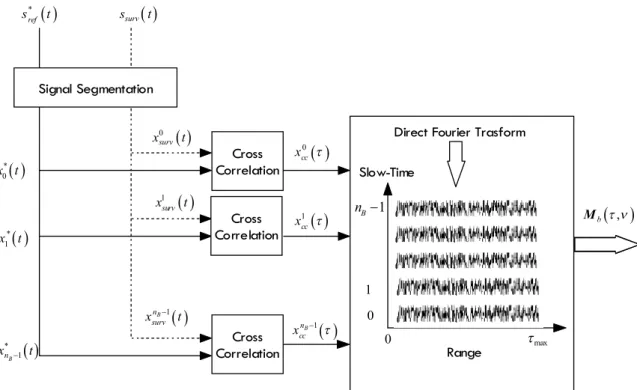
p h t h t as shown in Figure 1.1.   R s t   0 cc s  Slow-Time   p u t Range Signal Segm entation Cross Correlation Cross Correlation Cross Correlation   1 cc s    1 M cc s     0 R s t   1 R s t   1 M R s  t 0 PRI 1 M  0 1

Figure 1.1 Pulse radar architecture

The m-th matched filter output m

 

cc

s  is given by the cross correlation between the transmitted pulse u t_p

 

and the received signal collected into the m-th PRI m

 

R s t * 0 ( ) ( ) ( ) PRI m m cc R p s  



s t u    d (1.28)

After A/D converter, for each PRI, L range samples are collected to cover the range interval of interest. The received data for one CPI comprises LM complex baseband samples. This signal is the classical slow time-range bidimensional data.

Modeling the received signal, in the case of a single slowly fluctuating point target, as in equation (1.3)

(22)

 

_{2 Re}







i c Dat



R t a

s t _ E bu t_ e  

(1.29) the m-th matched filter output m

 

cc s  is given by

 

i DamTR *





 

i Dat m cc t p R a p s   E be



u t  mT  u t e dt (1.30)

Using equation(1.10), equation (1.30) can be modified as

 

1





0 , Da R M i mT m cc t p a Da m s  E b  e      



  (1.31)

where    is the ambiguity function of the single pulse.p



,



The output of the matched filter receiver for the m-th pulse is the ambiguity function of the transmitted pulse scaled and shifted on the time delay corresponding to the location of the target and calculated at the target Doppler frequency. Comparing equation (1.31) with equation (1.11) we can observe that we have some losses related to the target Doppler shift. This fact can be explaining considering that the filter is matched to only the target delay and not to the target Doppler frequency.

Consider only the target range gate the samples from each PRI are given by

 

i DamTR



0,



i DamTR

m

cc a t p Da

s   E be   _e (1.32)

where we have assumed that the waveform is insensitive to target Doppler shift and the other terms have been groped into a single complex random amplitude  .

The slow-time snapshot for the target range cell can be written as

 





_1; i Da RT _;...; i DaM 1TR cc a t Da e e    _  _  _    s v (1.33)

where v_t



_Da



is the so called temporal steering vector. It is a Vandermonde form because the waveform is a uniform PRF and the target velocity is supposed constant. The theory developed in the previous section can be applied in this case defining the vector s , shown in equation (1.13), equal to the temporal steering vector₀ vt



Da



. The

well known adaptive temporal (Doppler-Pulse) processing techniques, i.e. Moving Target Indicator (MTI) or Adaptive Moving Target Indicator (AMTI), are based on this consideration. In chapter 3 and 4 we will see how this analysis may be extended to the passive radar scenario.

(23)

So far we have considered the receiver system composed by only a single receiver, now we extend the development to a radar antenna consisting of N elements.

The single sensor signal model defined in equation (1.31) can be modified as





 





ˆ _, _, , , a a n c Da R i i mT m c cc n t p a Da s E be e           k r r (1.34) where





ˆ _, a a  

k is a unit vector pointing in the



  angular direction and,



r is the n-th_n

array element vector position.

It is assumed that the transmitted waveform is narrowband and the relative delay term is insignificant within the complex envelope.

After A/D converter the received data for one CPI comprises LMN complex baseband samples. This signal is the classical slow time-range-antenna elements multidimensional data, typically known as CPI datacube as schematically shown in Figure 1.2..

Consider only the target range gate, as shown in equation (1.32), the target samples from each PRI are given by





  ˆ _, _, a a n c Da R i i mT m c cc a n s e e      _ k r ,r (1.35)

Examination of equation (1.35) shows that one exponential term depends on the spatial index n and the other depends on the temporal index m.

Range Bin 1 L Antenna element N Slow time-PRI M

Figure 1.2 CPI datacube

(24)

 





  0   1   1 ˆ _, _, ˆ _, _, ˆ _, _, , ; ;...; Da R a a a a a a N c c c Da R i mT m cc a s a a i i i i mT _c _c _c e e e e e                             k r k r k r s v (1.36)

where vs



 a, a



is the so called spatial steering vector.

The theory developed in the previous section can be applied in this case defining the vector s , shown in equation (1.13), equal to the spatial steering vector. The well₀

known adaptive spatial processing techniques, also known as adaptive beamforming technique, are based on this simple consideration. In chapter 5 we will see how this analysis may be extended to the passive radar scenario..

In the case of an airborne pulse radar the 1D temporal adaptive processing and 1D spatial adaptive processing have been extended to the so called Space Time Adaptive Processing (STAP) techniques. This techniques elaborates the received signal in a joint spatiotemporal domain for advanced clutter suppression. The need for joint space and time processing arises from the inherent two-dimensional nature of the ground clutter due to the platform motion.

In this contest the adaptive filter theory can be applied thinking that the received signal can be alternatively written as

 









 

_

_





1 1 , ; , ;...; , , , Da R Da R i M T i T cc a s a a s a a s a a t s Da a a e e                  _ _  s v v v v (1.37)

where v_{t s}



  _Da, ,_a _a



is the space-time steering vector, and defining the vector s ,0

shown in equation (1.13), equal to the space-time steering vector.

In chapter 6 we will see how this analysis may be extended to the passive radar scenario.

1.3 Main contributions to research

The main obvious problem of passive radars is the necessity to estimate a copy of the transmitted signal. Therefore the simpler PBR system requires two receiving channels in order to collect the reference signal and the surveillance signal and to perform the matched filter receiver. The main challenge in passive bistatic radars is to mitigate the

(25)

interference signal, such as the direct path interference and its multipath, on the surveillance channel.

The second chapter introduces a typical passive radar scenario and describes the defined signal model for both reference and surveillance channel. Moreover the chapter presents the typical signal processing chain used in a PBR system. The main blocks are represented by both the matched filter block and the interference suppression block. The scope of the last block is to mitigate and ideally to suppress the interference components received on the surveillance channel. It is worth noting that the main feature of the traditional PBR signal processing chain is the presence of the interference suppression block before the matched filter.

The matched filter processor serves two distinct purposes: to provide the necessary signal processing gain to allow detection of the target echo and to estimate the bistatic range and Doppler shift of the target. The output of the matched filter is the classical 2D cross correlation function, often called as Cross Ambiguity Function (CAF). The evaluation of the 2D cross correlation function can be computationally expensive and a large number of complex operations has to be performed which sets a strong limitation on real time processing. Sub optimum approaches can be exploited to reduce the computational cost if a small SNR degradation can be accepted.

The third chapter develops a comparative study between optimum and sub optimum methods in terms of computational load and SNR loss. A new detailed formulation of the sub optimum “batches algorithm” is proposed. The exact matched filter formulation for OFDM waveforms is derived and we reveal that this approach is similar to the batches algorithm considering the same small Doppler approximation. The analogies with the classical processing used in active pulse radar are underlined. This analysis constitutes the basis for the development and the adaptation of the classical adaptive signal processing techniques, developed for active pulse radars, to a passive radar scenario.

(26)

The cancellation of the interference signal is a crucial issue for target detection in a passive bistatic scenario. Different techniques, both in spatial and temporal domain, have been proposed to solve this problem.

The forth chapter deals with the suppression of the direct signal and clutter echoes in a single receiver passive radar scenario. A variety of temporal adaptive processing has been developed for the removal of the interference component in the surveillance channel before the matched filter. A new formulation of the adaptive matched filter based on the “batches algorithm” is derived. The main advantage of the adaptive matched filter solution is the possibility to suppress strictly static clutter potentially affected by ICM (Internal Clutter Motion). The effectiveness of the proposed solution is demonstrated considering both simulated and real data.

Simpler passive bistatic radar systems use only two antennas for the reception of both surveillance and reference signal. Using a phased array antenna it is possible to electronically steer multiple beams at the same time to collect reference and surveillance channel and improve the target localization process. Typically digital beamforming techniques are applied directly on the received signal and before the matched filter.

The fifth chapter introduces the main advantages of a multichannel passive radar system implementing digital beamforming techniques. The main drawbacks of the mentioned traditional solution are detailed and a new scheme, based on the application of digital adaptive beamforming after matched filter, is investigated. The proposed technique improves the performances in terms of clutter cancellation on the surveillance channel. Once defined a multichannel signal model the effectiveness of the proposed solution has been demonstrated on simulated data.

In presence of a moving PBR, as in moving platform active radars, the clutter spectrum exhibits an angular direction–dependent mean frequency. Target detection realized by filtering the clutter in the frequency Doppler domain is difficult with a single antenna. An improvement in clutter suppression can be achieved by using an antenna array and

(27)

two-dimensional signal processing. Space-Time adaptive processing is typically used to filter out interferences in GMTI radars in order to detect slow moving target.

The sixth chapter demonstrates the applicability of STAP processing to passive bistatic radars. In the STAP literature, it is assumed that the available signal is formed by the echoes from a pulse-Doppler radar. A PBR system operates in a continuous mode, therefore the received signal is not avalaible in the classical array elements- slow time-range domain such as in an active pulse radar. The chapter introduces how the 1D temporal and spatial adaptive techniques can be extended to the 2D STAP processing and shows how the classical STAP algorithms, developed for active radar systems, can be applied to a PBR system.

(28)

Chapter 2. Signal

processing

techniques

in

passive radar systems

2.1 Introduction

In this chapter we introduce the signal processing techniques typically adopted in a PBR system. The principal block is represented by the matched filter. In section 2.2 we define the simpler PBR matched filter architecture by using the concepts developed in section 1.2.1. The matched filter is the optimum receiver in presence of additive white noise. A typical PBR scenario is more complex and this simpler structure presents several drawbacks. In section 2.3 the adopted model, for both reference signal and received signal and a typical passive bistatic scenario is described. The PBR environment will be presented and the main problems relative to a basic matched filter architecture will be underlined. In section 2.4 we will present an advanced signal processing architecture used in a typical PBR scenario. The main block introduced is the interference suppression block before the matched filter. The scope of this block is that to mitigate and ideally to suppress below the noise floor the several interference components received on the surveillance channel.

2.2 PBR matched filter architecture

The theory developed in section 1.2.1 explains that a PBR receiver requires at least two signals in order to perform the matched filter receiver: a copy of the transmitted signal

(29)

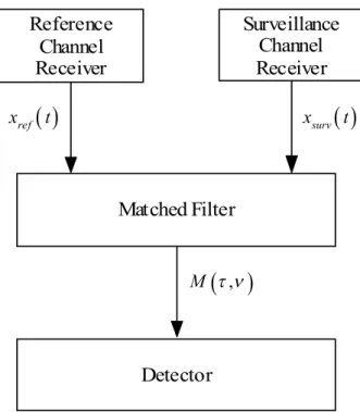
and the received signal from the surveillance area. The principal obvious potential problem of non-cooperative passive radar is that there is no copy of the transmitted signal at the receiver. This problem is important for every bistatic configuration but it becomes relevant for passive configuration because the transmitter is non-cooperative. Generally these two signals are addressed as surveillance channel, for the reception from the area of interest, and reference channel, which provides a reference for correlation based matched filter. The PBR matched filter receiver is shown in Figure 2.1. Reference Channel Receiver Surveillance Channel Receiver

 

ref x t x_surv

 

t Matched Filter

 

, M   Detector

Figure 2.1 Block diagram of the PBR matched filter

The simpler PCL radar system requires two antennas: the first antenna, often called the

reference antenna, is used to capture a direct version of the signal being utilised and

should point in the direction of the transmitter, the second antenna, usually called the

surveillance antenna, is used to capture the signals of potential target.

The output of the matched filter block is obtained as

 

  

*



2 0 , CUT T j t surv ref M   



x t x t e dt (2.1)

(30)

where M

 

  denotes the range–Doppler cross-correlation surface,, xsurv

 

t is the

echo signal and xref

 

t is the reference signal, delayed by an amount  seconds and

Doppler shifted by Hz.

The cross correlation function at the matched filter output is achieved by correlating the surveillance signal xsurv

 

t with Doppler-shifted versions of the reference signal xref

 

t

to form a bank of filters matched to every possible Doppler frequency of interest. The matched filter stage serves two important purposes:

the generation of sufficient signal processing gain to allow the targets to be detected above the noise floor

the estimation of the bistatic range and bistatic Doppler shift of the target echoes. In this first section we assume an ideal scenario in which we can perfectly capture the transmitted signal and the surveillance channel is composed by only target and thermal noise component. Based on this assumption the complex envelope of the total signal received in the reference channel x_ref

 

t and in the surveillance channel x_surv

 

t are given by

 

1





2 1

 

1 - T surv

ref ref ref

i t T surv surv x t x t n t x t x t e  n t           (2.2)

where x t

 

is a copy of the transmitted signal, _ref is the complex amplitude relative to the reference channel, _surv is the complex amplitude relative to the surveillance channel, _{ is the target delay,}₁T

1T

 is the target Doppler frequency, and nref

 

t n, surv

 

t

are thermal noise components.

Using equation (2.2) in equation (2.1) the output of the matched filter can be written as





1









1 1

, T, T ,

ref surv out

M   _        n   (2.3)

The output of the matched filter receiver is ideally the ambiguity function of the transmitted signal, scaled and shifted to be centered on the time delay and Doppler shift corresponding to target location and velocity.

(31)

2.3 Signal modelling and interference environment in a passive bistatic

radar

In this section the adopted model, for both reference signal and received signal and a typical passive bistatic scenario is described paying particular attention to the definition and representation of different contributions within the received signals. The purpose of this section is to provide a review of the interference environment and its impact on the PBR matched filter architecture described in the previous subsection.

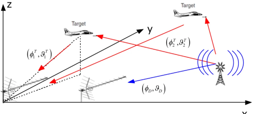
2.3.1 Single target geometry

In this first section we analyze the simpler scenario in which we have a single target and a single illuminator of opportunity. A typical passive radar single target geometry is shown in Figure 2.2. x y z



1 , 1



T T  



 D, D



Figure 2.2 Single target scenario

The reference and surveillance antennas are assumed to be collocated with the reference antenna steered toward the illuminator of opportunity and the surveillance antenna pointed in the direction to be surveyed.

Based on this assumption the complex envelopes of the total signal received in the reference channel xref

 

t and in the surveillance channel xsurv

 

t are given by

(32)

 





 





 

1 1 2 1 1 2 1 1 -T surv T surv i t T

ref ref ref

i t T

surv ref surv

x t x t x t e n t x t x t x t e n t          _ _ _       (2.4)

where x t

 

is a replica of the transmitted signal, _ref is the complex amplitude of the direct signal received via the main-lobe of the reference antenna, 1

1 1

, ,

surv T T

   are

respectively the complex amplitude, the delay with respect to the direct signal and the Doppler frequency shift of the target echo received via the side-back lobes of the reference antenna, _ref is the complex amplitude of the direct signal received via the side-back lobe of the surveillance antenna, 1

1 1

, ,

surv T T

   are respectively the complex amplitude, the delay with respect to the direct signal and the Doppler frequency shift of the target signal received via the mainlobe of the surveillance antenna,

 

,

 

ref surv

n t n t are respectively the thermal noise contribution at the reference and surveillance antenna.

We can observe that the terms 1 1

, , ,

surv ref surv ref

    are strictly related to the received target power P and the received direct power_t P ._d

The bistatic radar equation gives the target power received in the surveillance channel as





  



2 1 1 3 2 , 4 T T b surv t T R ERP G P R R       (2.5)

where ERP is the effective radiated power from the illuminator of opportunity,  is the_b target bistatic radar cross-section,



₁T, ₁T



surv

G   is the reference antenna gain respect to the angular direction



_{ }₁T, ₁T



_{of the surveillance area,}

T

R is the transmitter to target

distance, R is the target to receiver distance and the propagation losses have been_R

supposed negligible.

The power received directly from the transmitter of opportunity in the surveillance channel is





   

2 3 2 , 4 surv D D d ERP G P L      (2.6)

(33)

where ERP is the effective radiated power from the transmitter,



 _D, _D



are respectively the azimuth and elevation angles that defines the illuminator angular position, G_surv



 _D, _D



is the reference antenna gain respect to the angular direction



 _D, _D



of the illuminator of opportunity, L is the transmitter to receiver distance. The

target signal to direct signal ratio SDR in the surveillance channel is therefore





 









2 1 1 2 , , T T b surv t surv d T R surv D D G L P SDR P _{R R} _G        (2.7)

With similar considerations the SDR in the reference channel can be evaluated as





 









2 1 1 2 , , T T b ref t ref d _T _R _ref _D _D G L P SDR P R R G        (2.8) where



₁T, ₁T



ref

G   is the reference antenna gain respect to the direction of the surveillance area and G_ref



 _D, _D



is the reference antenna gain respect to the angular direction of the transmitter.

In typically scenarios the SDR can assume values between



90dB 70dB



as shown in the several references.

Assume the contribution of the target signal in the reference channel is negligible, equation (2.4) becomes

 

1





2 1

 

1 - T surv

ref ref ref

i t T

surv ref surv

x t x t n t x t x t x t e  n t         _ _ _  (2.9)

Using equation (2.9) in equation (2.1) the output of the matched filter can be written as





 

1









1 1

, 0,0 T, T ,

ref ref ref surv out

M   _           n   (2.10)

The presence of the direct signal in the surveillance channel causes any unwanted contributions at the output of the matched filter. The main contribution is confined to the zero-Doppler and zero range bin but the range and Doppler sidelobes of this autocorrelation function could remain significant.

The target to direct signal ratio at the output of the matched filter is proportional to the

surv

(34)

surveillance antenna are not comparable with the SDR_surv the target could be masked by the direct signal.

2.3.2 Multi target geometry

Considering the presence of N targets in the scenario, as shown in Figure 2.3, we can_T

extend the single target model as

 





 





 

2 1 2 1 -T _T m surv T _T m surv N i t m T

ref ref m ref

n N i t m T surv m surv n x t x t x t e n t x t x t e n t                 _ _ 



(2.11)

where x t

 

is a replica of the transmitted signal, _ref is the complex amplitude of the direct signal received via the main-lobe of the reference antenna, , ,

surv m T T

m m

   are

respectively the complex amplitude, the delay with respect to the direct signal and the Doppler frequency shift of the m-th target, , ,

surv m T T

m m

   are respectively the complex amplitude of the m-th target signal received via the mainlobe of the surveillance antenna, the m-th target delay with respect to the direct signal and the m-th target Doppler frequency shift,

 

,

 

ref surv

n t n t are respectively the thermal noise contribution at the reference and surveillance antenna.

x

y

z



1 , 1



T T  



 D, D





 2T, 2T



(35)

Note that the contribution of the direct signal component in the surveillance channel is not considered in this section because we have analyzed this component in the previous section. Assume the contribution of the target signal in the reference channel is negligible, equation (2.11) can be written as

 





2

 

1 T _T m surv

ref ref ref

N i t m T surv m surv m x t x t n t x t x t e  n t          _ _ _  



(2.12) Using equation (2.12) in equation (2.1) the output of the matched filter is













1 , T , , surv N m T T ref m m out m M          n      



 (2.13)

As we can see from equation (2.13) the matched filter receiver is not optimum when more than one moving target echo is present in the received signal. To understand this we can think to a simplified scenario. Let us assume that only two target are present in the received signal: one strong echo originating from a nearby target and one weak echo originating from a far target. The amplitudes of the ambiguity functions relative to the two target will be related to the amplitudes of the two received signals. Therefore the ratio between the two target power, at the output of the matched filter, will be proportional to the ratio

surv surv strong weak   (2.14)

In this case the detection of the first target will be performed almost perfectly while detection of the weak echo could be very difficult or impossible.

This event typically occurs when a specular reflection is observed on a large jet aircraft, or when a target passes very close to the transmitter or receiver. In this case, the range and Doppler sidelobes of this large return can be sufficient to mask the other, smaller target returns on the correlation surface. [Kulpa 2005] propose the iterative removal of such returns by estimating their position in range–Doppler, and then adaptively filtering them from the original data, before recalculating the correlation surface. The approach can be repeated for every strong return, but at the expense of non real-time operation in some instances.

(36)

2.3.3 Multipath environment

In the precedent sections we have assumed that the received signal in the reference channel and in the surveillance channel is free to multipath. In an actual application this assumption will not be fulfilled and the received signal consists of more terms originating from the reflections of the transmitted power from distributed objects.

The typical baseband complex envelope model for the multipath channel is

 

0

 





 

1 -C n N i rx n m n x t  x t  e x t  n t   



 (2.15) where

 

rx

x t is the received signal

 

x t is a delayed replica of the transmitted signal

0

 is the complex amplitude of the direct signal

C

N is the number of paths

, ,

m m m

   are respectively the amplitude, the phase and the delay with respect to the direct signal of the m-th path

 

n t is the thermal noise contribution

This model is widely accepted in open literature relative to radio communication applications and it is used in all works about passive radar systems.

The received signal expressed in equation (2.15) can be seen as the sum of different contributions relative to a set of small discrete stationary scatterers. A continuous backscattering environment can be emulated by utilizing a large number of such scatters. Different criteria can be adopted to set the positions and the backscattering characteristics of the scatterers which determine the delays and amplitudes of the correspondent echoes.

A widely accepted statistical model in the radio communication community, as defined in the standard DVB-T ETSI [ETSI 2009] assume the following distributions:

the amplitude term  relative to each path is assumed to have a Rayleigh distribution

 

2 22

 

1 exp 2 i i f   u       _ _   (2.16)

Space time adaptive processing in multichannel passive radar

UNIVERSITÀ DI PISA

Scuola di dottorato in Ingegneria “Leonardo da Vinci”

Corso di Dottorato di Ricerca in

TELERILEVAMENTO

Tesi di Dottorato di Ricerca