Third generation neural networks: formalization as timed automata, validation and learning

A

LMA

M

ATER

S

TUDIORUM

·

U

NIVERSIT

A DI

`

B

OLOGNA

SCUOLA DIINGEGNERIA EARCHITETTURA

Corso di Laurea Magistrale in Ingegneria e Scienze Informatiche

Third generation neural networks:

formalization as timed automata,

validation and learning

Tesi in:

Linguaggi Di Programmazione E Modelli Computazionali

Relatore:

Chiar.mo Prof. Gianluigi Zavattaro

Correlatori:

Dott.ssa Cinzia Di Giusto

Dott.ssa Elisabetta De Maria

Presentata da:

Giovanni Ciatto

Sessione III

A.A. 2015/2016

Abstract. In questa tesi viene mostrato come le reti neurali spiking, note an-che come reti neurali di terza generazione, possano essere formalizzate us-ando reti di automi temporizzati. Tali reti neurali, a differenza di quelle di sec-onda generazione (e.g. reti multilivello con funzione di attivazione sigmoidale), considerano anche la dimensione temporale nell’evoluzione della loro com-putazione. Sono mostrate due possibili formalizzazioni, sincrona e asincrona, del modello di neurone “discrete leaky integrate and fire”: in entrambi i casi, i neuroni sono modellati come automi temporizzati che restano in attesa di impulsi su un dato numero di canali di ingresso (sinapsi) per poi aggiornare il proprio potenziale tenendo conto degli input presenti e passati, opportuna-mente modulati dai pesi delle rispettive sinapsi e tanto pi `u influenti quanto pi `u recenti. Se il potenziale corrente supera una certa soglia, l’automa emette un segnale broadcast sul suo canale di uscita. Dopo ogni emissione, gli automi sono vinciolati a rimanere inattivi per un periodo refrattario fissato, alla fine del quale il potenziale `e azzerato. Nel modello asincrono, si assume che gli impulsi in ingresso siano molto frequenti ma se ne impone l’ordinamento: non sono ammessi ingressi contemporanei. Nel modello sincrono, tutti gli impulsi ricevuti all’interno del medesimo periodo di accumulazione sono considerati simultanei. Una rete di neuroni `e ottenuta eseguendo in parallelo pi `u automi: questi devono condividere i canali in maniera da riflettere la struttura della rete. Le sequenze di impulsi da dare in pasto alle reti sono a loro volta speficate tramite automi temporizzati. `E possibile generare tali automi per mezzo di un procedimento automatico, a partire da un linguaggio, appositamente definito, che modella sequenze, al pi `u infinite, di impulsi e pause. Il modello sincrono `e validato rispetto alla sua capacit `a (e incapacit `a) di riprodurre alcuni com-portamenti (relazioni tipiche tra ingressi e uscite) ben noti in letteratura. La formalizzazione basata sugli automi temporizzati `e poi sfruttata per trovare un assegnamento per i valori dei pesi sinaptici di una rete neurale in maniera da rendere quest’ultima capace di riprodurre un comportamento dato, espresso da una formula di logica temporale. Tale risultato `e raggiunto per mezzo di un algoritmo che, previa identificazione degli errori commessi dai neuroni di output nel produrre l’uscita attesa, permetta di applicare delle azioni tive sui pesi delle loro sinapsi in ingresso. Le informazioni sulle azioni corret-tive adeguate vengono poi propagate all’indietro verso gli altri neuroni della

presentati: uno basato sulla simulazione e uno basato sul model-checking.

Keywords: Spiking neural networks, timed automata, supervised learning, CTL, model-checking

v

Acknowledgments

This thesis is the result of a six-months internship at the I3S laboratory of the University of Nice–Sophia Antipolis (France), which I consider a life-changing experience.

I wish to thank Prof. Gianluigi Zavattaro for offering me such a great op-portunity, for his support, for his trust in me and my capabilities.

I wish to thank Prof. Cinzia Di Giusto and Prof. Elisabetta De Maria for supervising my work, supporting me in a foreign country, and for the so many things I have learned about theoretical informatics and academic life. A spe-cial acknowledgment goes to Prof. Di Giusto for her patience and persever-ance, for her precious suggestions, critics, encouragements, and the for ran-dom thoughts we shared.

I wish to thank my new friends Selma Souihel and Marco Benzi for the so many times we had fun together, for their company and their support, and for sharing their cultures with me. I sincerely hope we will eventually meet again.

I wish to thank my friends and colleagues Massimo Neri and Federico Fucci, the former for indirectly being the cause of such an adventure, and the latter for writing me almost everyday keeping alive my connection with the beloved city of Cesena.

Finally, I wish to thank my parents, Anna and Carmelo, and my sister Irene, for always supporting me and my decisions both emotionally and economically. I owe them everything and it is thanks to them if I did it this far.

Contents

Abstract

iii

Acknowledgments

v

1

Introduction

1

2

Theoretical background

7

2.1 Neural networks . . . .

7

2.1.1

Leaky-integrate-and-fire model . . . .

12

2.2 Supervised and unsupervised learning with SNNs

14

2.3 Timed automata . . . .

17

2.4 Formal verification . . . .

23

3

Spiking neural network formalization

27

3.1 LI&F neurons as timed automata . . . .

27

3.1.1

Asynchronous encoding as timed automata

28

3.1.2

Synchronous encoding as timed automata .

31

3.2 SNNs as timed automata networks . . . .

34

3.2.1

Handling networks inputs . . . .

35

3.2.2

Handling networks outputs . . . .

41

3.3 Implementing SNNs in

Uppaal

. . . .

42

4

Validation of the synchronous model

49

4.1 Intrinsic properties . . . .

51

4.2 Capabilities

. . . .

56

4.3 Limits . . . .

62

5

Parameters tuning and learning

77

5.1 Learning problem for synchronous SNNs

. . . . .

78

5.2 Simulation-oriented ABP . . . .

84

5.3 Model-checking-oriented ABP

. . . .

95

6

Conclusions and future works

99

Chapter 1

Introduction

Researchers have been trying to reproduce the behavior of the brain for over half a century: on one side they are studying the inner functioning of neurons — which are its elementary components —, their interactions and how such aspects participate to the ability to move, learn or remember, typical of living beings; on the other side they are emulating nature trying to reproduce such capabilities e.g., within robot controllers, speech/text/face recognition applica-tions etc.

In order to achieve a complete comprehension of the brain functioning, both neurons behavior and their interaction must be studied. Historically, inter-connected neurons, “neural network”, have been naturally modeled as directed weighted graphs where vertices are computational units receiving inputs by a number of ingoing arcs, called synapses, elaborating it, and possibly propa-gating it over of outgoing arcs. Several inner models of the neuron behavior have been proposed: some of them make neurons behave as binary threshold gates, other ones exploit a sigmoidal transfer function, while, in a number of cases, differential equations are employed.

According to [24, 27], three different and progressive generations of neural networks can be recognized: (i) first generation includes discrete and thresh-old based models (e.g., McCulloch and Pitt’s neuron [25]); (ii) second genera-tion consists of real valued and sigmoidal-based models, which are nowadays heavily employed in machine learning related tasks because of the existence of powerful learning algorithms (e.g., error back-propagation [29]); (iii) third

generation, which is the focus of our work, consists of a number of models that, in addition to stimuli magnitude and differently from previous generations, take time into account.

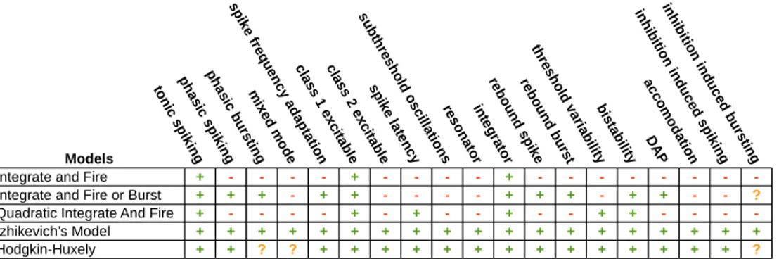
Models from the third generation, also known as “spiking neural networks”, are weighted directed graphs where arcs represent synapses, weights serve as synaptic strengths, and vertices correspond to “spiking neurons”. The latter ones are computational units that may emit (or fire) output impulses (spikes) taking into account input impulses strength and their occurrence in-stants. Models of this sort are of great interest not only because they are closer to natural neural networks behavior, but also because the temporal dimension allows to represent information according to various coding schemes [27, 28]: e.g., the amount of spikes occurred within a given time window (rate coding), the reception/absence of spikes over different synapses (binary coding), the relative order of spikes occurrences (rate rank coding) or the precise time difference between any two successive spikes (timing code). A number of spiking neuron models have been proposed into the literature, having different complexities and capabilities. In [21] spiking neuron models are classified ac-cording to some behaviors (i.e., typical responses to an input pattern) that they should exhibit in order to be considered biologically relevant. For example the leaky-integrate-and-fire (LI&F) model [22], where past inputs relevance expo-nentially decays with time, is one of the most studied neuron models because of its simplicity [21, 27], while the Hodgkin-Huxley (H-H) model [18] is one of the most complex and important within the scope of computational neuro-science, being composed by four differential equations comparing the neuron to an electrical circuit. For instance, two behaviors that every model is able to reproduce are the tonic spiking and integrator : the former one describes neurons producing a periodic output if stimulated by a persistent input, the lat-ter one illustrates how temporally closer input spikes have a grealat-ter excitatory effect on neurons potential, making them able to act as coincidence detectors. As one may expect, the more complex the model, the more behaviors it can be reproduce, at the price of greater computational cost for simulation and formal analysis; e.g., the H-H model can reproduce all behaviors, but the simulation process is really expensive even for just a few neurons being simulated for a small amount of time [21].

3 Our aim is to produce a neuron model being meaningful from a biological point of view but also amenable to formal analysis and verification, that could be therefore used to detect non-active portions within some network (i.e., the subset of neurons not contributing to the network outcome), to test whether a particular output sequence can be produced or not, to prove that a network may never be able to emit, or assess if a change to the network structure can alter its behavior; or investigate (new) learning algorithms which take time into account.

In this work, we take the discretized variant of LI&F introduced in [13] and we encode it into timed automata. We show how to define the behavior of a single neuron and how to build a network of neurons. Finally, we show how to verify properties of the designed system via model-checking.

Timed automata are finite state automata extended with timed behaviors: constraints are allowed limiting the amount of time an automaton can remain within a particular state, or the time interval during which a particular transition may be enabled. Timed automata networks are sets of automata running in parallel and interacting by means of channels.

Our modeling of spiking neural network consists of a timed automata net-works where each neuron is an automaton alternating between two states: it accumulates the weighted sum of inputs, provided by a number of ingoing weighted synapses, for a given amount of time, and then, if the potential accu-mulated during the last and previous accumulation periods overcomes a given threshold, the neuron fires an output over the outgoing synapse. Synapses are channels shared between the timed automata representing neurons, while spike emissions are represented by synchronizations occurring over such chan-nels. Timed automata can be exploited to produce or recognize precisely de-fined spike sequences, too.

The biophysical behaviors mentioned above are interpreted as computa-tional tree logic (CTL) formulae and are tested in Uppaal [4] that provides an extended modeling language for automata, a simulator for step-by-step analy-sis and a subset of CTL for systems verification.

Finally, we exploit our automata-based modeling to propose a new method-ology for parameter learning in spiking neural networks, namely the advice back-propagation (ABP) approach. In particular, ABP allows to find an

as-signment for the synaptic weights of a given neural network making it able to reproduce a given behavior. We take inspiration from SpikeProp [8], a variant of the well known back-propagation algorithm [29] used for supervised learning in second generation networks. SpikeProp reference model takes into account multi-layered cycle-free spiking neural networks and aims at training them to produce a given output sequence for each class of input sequences. The main difference with respect to our approach is that we are considering here a dis-crete model and our networks are not multi-layered. We also rest on Hebb’s learning rule [17] and its time-dependent generalization, the spike-timing de-pendent plasticity (STDP) rule [30]: they both act locally, with respect to each neuron, i.e., no prior assumption on the network topology is required in order to compute the weight variations for some neuron input synapses. Differently from STDP, our approach takes into account not only the recent spikes but also some external feedback, the advices, in order to determine which weights should be modified and whether they must be increased or decreased. More-over, we do not prevent excitatory synapses from becoming inhibitory (or vice versa), which is usually a constraint for STDP implementations. A general overview on spiking neural network learning approaches and open problems in this context can be found in [16].

The rest of this thesis is organized as follows. Chapter 2 exposes the the-oretical background. It explains the differences between the three neural net-works generations and describes our reference model, the LI&F. It provides an overview over existing learning approaches within the context of second and third neural network generations. Then, it recalls definitions of timed au-tomata networks, CTL and model-checking. Chapter 3 shows how spiking neural networks are encoded into timed automata networks, how inputs and outputs are defined by means of an ad-hoc language and encoded into au-tomata, as well. Chapter 4 describes how we validated our formalized model by providing formal proofs for the behaviors listed above. It also discuss the intrinsic properties of our model, e.g., the maximum threshold or the lack of inter-spike memory. Then, a number of extension are proposed, aiming to en-dow our model with further capabilities, such as the ability to emit bursts. In chapter 5, we introduce the learning problem and our ABP approach from an abstract point of view. We then provide two possible ways to realize it: the first

5 one is simulation-oriented and the second one is model-checking-oriented. Fi-nally, chapter 6 summarizes our results and presents some future research directions.

Publications. This thesis has been the starting point for two scientific pa-pers. The first one [9], describing our formalization of leaky-integrate-and-fire neural networks, has been accepted by the ASSB student workshop. The second one, concerning our approach to the learning problem, has been sub-mitted to the international conference Coordination 2017.

Chapter 2

Theoretical background

In this chapter we present or recall a number of concepts which are discussed in the rest of this thesis.

We begin by describing a well established categorization of neural net-works within three consecutive generations, then we recall Maass’ widely gen-eral definition of spiking neural networks (i.e., a network from the third gener-ation) and present the discrete leaky-integrate-and-fire neuron model which is extensively discussed and exploited in the following chapters. We also provide an overview about supervised and unsupervised learning within the scope of spiking neural networks and we compare learning approaches between sec-ond and third generation neural networks.

Then, we recall the definition and semantics of timed automata and timed automata networks, which compose the conceptual framework we exploited the most in our spiking neural networks formalization proposal. Finally, we briefly present the definition of the CTL temporal logics, the model-checking problem, and we provide an intuition of their semantics.

2.1

Neural networks

Neural networks are directed weighted graphs were nodes are computational units, also known as neurons, and edges represents synapses, i.e., connec-tions between some neuron output and some other neuron input. Several models exist into the literature and they differ on the signals that neurons

emit/accept and on the way such signal are elaborated. An interesting classi-fication has been proposed in [24] which distinguishes three different genera-tions of neural networks:

1. Network models within the first generation handle discrete inputs and outputs and their computational units are threshold-based transfer func-tions; this includes McCulloch and Pitt’s threshold gate [25], the percep-tron [15], Hopfield networks [19] and Boltzmann machines [2].

2. Second generation models, instead, exploit real valued activation func-tions, e.g., the sigmoid function, accepting and producing real values: a well known example is the multi-layer perceptron [11, 29]. According to a common interpretation, the real-valued outputs of such networks represents the firing rates of natural neurons [27].

3. Networks from the third generation are known as spiking neural net-works. They extend second generation models treating time-dependent and real valued signals often composed by spike trains. Neurons may fire output spikes according to threshold-based rules which take into ac-count input spikes magnitude and occurrence time [27].

The core of our analysis are spiking neural networks. Because of the intro-duction of timing aspects (in particular, observe that information is represented not only by spikes magnitudes but also by their occurrence timings) they are considered closer to the actual brain functioning than models from previous generations.

We adopt Maass’ definition (see [24] or [23]) because it is a widely gen-eral template which can be specialized in more fine-grained characterizations by providing additional constraints. Spiking neural networks are modeled as directed weighted graphs where vertices are computational units and edges represents synapses. The signals propagating over synapses are trains of impulses: spikes. The particular wave form of impulses must be specified by model instances. Synapses may modulate such signals according to their weight or they could introduce some propagation delay. Synapses are clas-sified according to their weight as excitatory, if it is positive, or inhibitory if negative.

2.1. NEURAL NETWORKS 9 Computational units represents neurons, whose dynamics is governed by two variables: the membrane potential (or, simply, potential) and the thresh-old. The former one depends on spikes received by neurons over ingoing synapses, after being modulated and/or delayed. Both current and past spikes are taken into account even if old spikes contribution is lower. The latter may vary according to some rule specified by instances. The neuron outcome is controlled by the algebraic difference between the membrane potential and the threshold: it is enabled to fire (i.e., emit an output impulse over all outgo-ing synapses) only if such difference is non-negative. Immediately after each emission the neuron membrane is reset.

Another important constraint, typical of spiking neural networks, is the re-fractory period : each neuron is unable to fire for a given amount of time after each emission. Such behavior can be modeled preventing the potential to reach the threshold either by keeping the former low or the latter high.

More formally:

Definition 2.1 (Spiking neural network). Let E = {f | f : R+0 → R} be the set

of functions from continuous time to reals, then a spiking neural network is a tuple (V, A, ε), with:

• V is the set of spiking neurons, • A ⊆ V × V is the set of synapses,

• ε : A → E is function assigning to each synapse (u, v) ∈ A a response function εu,v ∈ E.

We distinguish three disjoint sets Viof input neurons, Vintof intermediary

neu-rons, and Voof output neurons, with V = Vi∪ Vint∪ Vo.

Definition 2.2 (Spiking neuron). A spiking neuron v is a tuple (θv, pv, τv, yv),

where:

• θv ∈ E is the threshold function,

• pv ∈ E is the [membrane] potential function,

• yv ∈ E is the outcome function.

The dynamics of a neuron v is defined by means of the set of its firing times Fv = {t1, t2, . . .} ⊂ R+0, also called spike train. Such set is defined

recursively: ti+1 is computed as a function of the value yv(t − ti), i.e., the

outcome of v since the instant ti. For instance, a trivial model may consider

yv(t − ti) to be greater than 0 for the instant tspike, defined as the smallest t

such that pv(t − ti) ≥ θv(t − ti). Analogously, in a stochastic model, the value

yv(t − ti) may govern the firing probability for neuron v.

The after-spike refractory behavior is achieved by making it impossible for the potential to reach and overcome the threshold. This can be modeled in two ways: (i) making any neuron unable to reach the threshold, e.g., by con-straining each threshold function θv such that: θv(t − t0) = +∞ if t − t0 < τv

for each t0 ∈ Fv; (ii) making any neuron ignore its inputs, e.g., by constraining

each potential function pvsuch that: pv(t − t0) = 0 if t − t0 < τvfor each t0 ∈ Fv,

Each response function εu,v represents the impulse propagating from

neu-ron u to neuneu-ron v and can be used to model synapse-specific features, like delays or noises. For instance, a model may allow signals to be modulated and delayed by defining εu,v as follows:

εu,v(t) = wu,v · yu(t − du,w)

where wu,v is a synaptic weight representing the strength of the synapse

(u, v), and du,v is the propagation delay introduced by such a synapse.

For each neuron v ∈ Vint∪ Vo, the potential function pv takes into account

the response function value εu,v(t − t0), for each previous or current firing time

t0 ∈ Fv : t0 ≤ t and for each input synapse (u, v); so the current potential may

be influenced by both the current and the previous inputs. For each neuron v ∈ Vi, the set Fv is assumed to be given as input for the network. For all

neuron v ∈ Vo, the set Fv is considered an output for the network.

Such a definition is deliberately abstract because there exist into the lit-erature a number of models fitting it, differing in the way they handle e.g., potentials, signal shapes, etc.

Some authors [21,27] classify the models presented in literature according to their biophysical plausibility. Estimating such a feature for a given model

2.1. NEURAL NETWORKS 11

(a) Tonic Spiking (b) Excitability (c) Integrator

Figure 2.1: Summary and graphical representation of some of the most interesting neuron behaviors we mention within this thesis, taken from [21]. Each cell shows the neuron response (in the upper part) to a particular input current (in the lower part).

Figure 2.2: Comparison between several neuron models taking into account the amount of behaviors from figure 2.1 the model can reproduce. See [21] for more detailed descriptions and for references.

may be a complex task since it is not well formalized. According to Izhikevich, there exists a set of behaviors, some shown in figure 2.1, which a neuron may be able to reproduce. A behavior is basically a well-featured input-output relation and a model is said to be able to reproduce it if there exists at least one instance of the model presenting a comparable outcome when receiving an alike input. The author also proposes to use the amount of behaviors a model can reproduce as a measure of its biophysical plausibility.

As far as our work is concerned, the most interesting results are about the integrate-and-fire model capabilities. Indeeds, instances of this model should be able to reproduce the following behaviors:

Tonic spiking: as a response to a persistent input, the neuron periodically

fires spikes as output.

magnitude.

Integrator: a neuron of this sort prefers high-frequency inputs: the higher

the frequency the higher its firing probability; it may act as inputs coinci-dence detector.

2.1.1

Leaky-integrate-and-fire model

Since our aim is to define a model being simple enough to be inspectable through model-checking techniques but also complex enough to be biophys-ically meaningful, we focused on the leaky-integrate-and-fire (LI&F), which is one of the simplest and most studied model of biological neuron behavior (see [21] and [27]), whose original definition is traced back to [22].

We adopt the formulation proposed in [13]. It is a discretized model, amenable to formal verification, where time progresses discretely, signals are boolean-valued even if potentials are real-boolean-valued, thresholds are constant over time and potentials vary according to both the currently and previously received spikes. Synapses do not introduce any delay. They instantaneously propagate the spikes from the producing neurons to the consuming ones, modulating them according to their weight.

Definition 2.3 (LI&F network). A leaky-integrate-and-fire network (V, A, W )

is a particular case of spiking neural network (V, A, ε), where:

• V = Vi∪ Vint∪ Vois the set of neurons such that each v ∈ Vint∪ Vois a

leaky-integrate-and-fire neuron,

• A ⊆ V × V is the set of synapses such that (v, v) /∈ A, ∀v ∈ V ,

• W : A → R is the weight function assigning to each synapse (u, v) a weight wu,v = W (u, v) ∈ [ −1, 1 ] such that the response functions

assigned by ε share the form:

εu,v(t) = wu,v · yu(t)

Definition 2.4 (LI&F neuron). A leaky-integrate-and-fire neuron v = (θ(0)v , λv,

2.1. NEURAL NETWORKS 13 • θv(0)∈ R is the constant threshold value, such that θv(t) = θ

(0) v , ∀t,

• λ ∈ [0, 1] is the leak factor,

• pv : N → R is the potential function, defined as

pv(t) =

X

(u, v)∈A

εu,v(t) + λv· pv(t − 1) (2.1)

where pv(0) = 0,

• τv ∈ N+is the refractory period duration,

• yv : N → {0, 1} is the outcome function, defined as

yv(t) =    1 if pv(t) > θv 0 otherwise (2.2) We refer to the value εv(t) =

P

(u, v)∈Aεu,v(t) as the sum of weighted inputs

of neuron v at time unit t, because, according to definition 2.3, the following equivalence holds true:

εv(t) =

X

(u, v)∈A

wu,v· yu(t)

Thus, we can rewrite equation 2.1 in a more concise way:

pv(t) = εv(t) + λv · pv(t − 1) (2.3)

From the point of view of the consuming neuron v, we say that, whenever yu(t) = 1 for some u, an input spike propagates, occurs or is received over the

synapse (u, v). From the point of view of the producing neuron u, we say that, whenever yu(t) = 1, the output spike propagates, occurs or is sent over the

synapses (u, v), for all v. Synapses do not introduce any propagation delay, but they modulate the spikes according to their weights. A synapse (u, v) is said to be excitatory if wu,v ≥ 0, inhibitory otherwise.

Finally, let tf be the last time unit where v emitted a spike, i.e., yv(tf) = 1,

then, for a given refractory period τv ∈ N, pv(tf+ k) = 0, ∀k < τ . Please note

that during any refractory period: (i) the neuron cannot increase its potential; (ii) it cannot emit any spike, since pv(tf + k) < θv; (iii) any received spike is

Remark. There exists an explicit version for equation 2.3, that is1: p(t) = t X k=0 λk· ε(t − k) (2.4) which clearly shows how previous inputs relevance exponentially decays as time progresses. Such formulation is achieved as follows:

p(0) = ε(0) = λ0 · ε(0) p(1) = ε(1) + λ · p(0) = λ0 · ε(1) + λ1_{· ε(0)} p(2) = ε(2) + λ · p(1) = λ0 · ε(2) + λ1_{· ε(1) + λ}2_{· ε(0)} p(3) = ε(3) + λ · p(2) = λ0 · ε(3) + λ1_{· ε(2) + λ}2_{· ε(1) + λ}3_{· ε(0)} .. . p(t) = ε(t) + λ · p(t − 1) = Pt k=0λk· ε(t − k)

2.2

Supervised and unsupervised learning with

spiking neural networks

In this section we provide an overview about learning approaches within the context of (spiking) neural networks.

Neural network models often rely upon a number of parameters, e.g., in definitions 2.3 and 2.4 we introduce synaptic weights, thresholds, leak factors, and refractory periods. By “learning”, we mean the process of searching for an assignment of such parameters according to a given criterion. To the best of our knowledge, all the criteria presented into the literature focus on the synaptic weights instead of the whole gamma of parameters employed by their respective reference models.

Traditionally, learning approaches are categorized as supervised or unsu-pervised. In a supervised learning process, the network is fed by a number of inputs and its outcome is compared with an equal number of expected out-puts. In this case, parameters are varied trying to minimize the difference between the actual and the expected outputs. Well known approaches to su-pervised learning are, for instance: error back-propagation, [29], for second

2.2. SUPERVISED AND UNSUPERVISED LEARNING WITH SNNS 15 generation neural networks, and its time-aware descendants, SpikeProp [8] and back-propagation-through-time (BPTT) [26], for spiking neural networks. Conversely, in an unsupervised learning process, inputs are not associated to any expected outcome, and the parameters of the network are varied in order to capture similarities or co-occurrences between patterns of inputs. Two well known rules, namely the Hebb rule [17] and its time-aware extension, spike-timing dependent plasticity (STDP) [30], were conceived as nature-inspired models of synaptic plasticity, i.e., synaptic strength variation rules, but they can also be considered unsupervised learning approaches, from a computa-tional point of view.

Back-propagation and its derivates. More than two decades ago, Rumel-hart et al. introduced the back-propagation algorithm [29], that is nowadays one of the most known and studied supervised learning approaches for net-works within the second generation [27].

Back-propagation assumes the network topology to be multi-layered, non-recurrent and feed-forward, i.e., neurons are organized in layers. Each ingoing edge comes from a neuron within the previous layer and each outgoing edge is directed to a neuron within the next layer. This is true for all but the first layer — containing the input neurons — and last one — containing output neurons. Being a supervised approach, a number of inputs are provided to the network, and its outcome is compared with the expected outputs. An error function, measuring the squared difference between actual and expected outputs with respect to the weights of the network, is minimized by descending its gradient at each step of the algorithm, i.e., the weights are varied in order to reduce the error currently performed by the network. Sadly, it cannot guarantee to reach the global minimum of such an error function, since it may get stuck within some local minima.

Several attempts of applying similar approaches to third generation neural networks have been proposed, e.g., SpikeProp [8] or BPTT [26]. The great-est obstacle when trying to adapt back-propagation to spiking neural networks is the inherently discontinuous nature of spikes and spiking neurons with re-spect to time. To overcome such a limitation, spikes are modeled by impulsive but still continuous functions, asymptotically decaying to zero. For instance,

SpikeProp employs the function ε(t) = t · ν−1 · e1−t/ν_{, where ν dictates how}

slowly impulses decay to zero. Another obstacle may be information represen-tation. Back-propagation is conceived for second generation neural networks, where inputs and outputs are represented by real numbers. As we outlined in chapter 1, there exist several ways to represent information by means of spikes, e.g., temporal, rate, count or rank coding [27]. Information represen-tation is an important trait when the actual and expected outputs come to be compared. Thus, supervised learning approaches within the scope of spiking neural networks must explicitly or implicitly assume a particular coding. For instance, SpikeProp employs temporal coding, i.e., the information carried by a spike is encoded by the time elapsed since the previous spike.

SpikeProp, too, exploits gradient descendant to minimize an error func-tion. The learning process affects both synaptic weights and synaptic delays, which are part of SpikeProp reference model. Another difference with back-propagation is that time differences between the actual and expected spikes are taken into account by such a function.

Hebbs rule and STDP. The principle behind all Hebb’s rule implementations is postulated in [17, p. 62]:

When an axon of cell A is near enough to excite a cell B and repeatedly or persistently takes part in firing it, some growth process or metabolic change takes place in one or both cells such that A’s efficiency, as one of the cells firing B, is increased.

For first and second generation networks, the following learning rule is classi-cally presented as an implementation of such a principle:

∆wi = η · xi· y

where ∆wi is the weight variation of the i-th input synapse for some neuron

N , η is the learning rate, xi is the value of the i-th input of N , and y is the

output of N . The rule states the synapse connecting two neurons must be strengthened proportionally to the product of the outputs of the two neurons.

STDP is considered the time-dependent counterpart of Hebb’s rule for spiking neural networks [27, 30]. It is strongly believed [7, 12] that the weight

2.3. TIMED AUTOMATA 17

Δw

Δt

(a) Greater variation for smaller ∆t. Symmetric for ∆t > 0 and ∆ < 0.

Δw

Δt

(b) Greater variation for smaller ∆t. Asymmetric for ∆t > 0 and ∆ < 0.

Δw

Δt

(c) Smaller variation for near-zero and greater ∆t. Asymmetric for ∆t > 0 and ∆ < 0. Δw Δt (d) Strengthening for smaller |∆t|, weakening for greater |∆t|.

Figure 2.3: Window functions patterns for STDP, from [27]. In the three cases 2.3a, 2.3b and 2.3c, the synapse is strengthened for positive ∆t and weakened otherwise.

variation of a synapse is strictly correlated with the relative timing of the post-synaptic spike with respect to the pre-post-synaptic one. From the point of view of a synapse (u, v), the pre-synaptic spike is the one emitted by neuron u at time tpre, and the post-synaptic spike is the one emitted by v at time tpost. As

summarized in [27], the general formulation of STDP is: ∆wu,v = f (∆t)

where ∆wu,v is the weight variation of synapse (u, v), ∆t = tpost− tpre, and

f is a window function, i.e., a smoothed function matching one of the patterns in figure 2.3. Such a rule states the weight of a synapse is varied accord-ing to the difference of occurrence times between the pre- and post-synaptic spikes. According to [30], the window function f is commonly implemented by means of pairs of negative exponential functions, built in such a way to prevent excitatory synapses to become inhibitory and vice versa.

2.3

Timed automata

Timed automata [3, 5] are a powerful theoretical formalism for modeling and verification of real time systems. Next, we recall their definition and semantics, their composition into timed automata networks as well as the composed net-work semantics. We conclude with an overview on the extension introduced by the specification and analysis tool Uppaal [4] that we have employed here.

A timed automaton is a finite state machine extended with real-valued clock variables. Time progresses synchronously for all clocks, even if they can be reset independently when edges are fired. States, also called locations, may be enriched by invariants, i.e., constraints on the clock variables limiting the amount of time the automaton can remain into the constrained location. Edges are enriched too: each one may be labeled with guards, i.e., constraints over clocks which enable the edge when they hold, and reset sets, i.e., sets of clocks that must be reset to 0 when the edge is fired. Symbols, optionally consumed by edge firings, are here called events. More formally:

Definition 2.5 (Timed automaton). Let X be a set of symbols, each identifying

one clock variable, and let G be the set of all possible guards: conjunctions of predicates having the form x o n or (x − y) o n, where x ∈ X, n ∈ N and o ∈ {>, >, =, 6, <}. Then a timed automaton is a tuple (L, l(0), X, I, A, E) where:

• L is a finite set of locations; • l(0) _{∈ L is the initial location;}

• I : L → G is a function assigning guards to locations; • A is a set of symbols, each identifying an event;

• E ⊆ L×(A∪{ε})×G×2X_{×L is a set of edges, i.e., tuples (l, a, g, r, l}0₎

where:

– l, l0 are the source and destination locations, respectively,

– a is an event, – g is the guard,

– r ⊆ X is the reset set.

In order to present de semantics of timed automata, we need to recall the definition of labeled transition systems, which are a formal way to describe formal systems semantics. They consist of directed graph where vertices are called states, since each of them represents a possible state of the source sys-tem, and edges are referred as transitions, since they represent the allowed

2.3. TIMED AUTOMATA 19 transitions, from a state to another, for the source system. Edges are deco-rated through labels representing, e.g., the action firing a particular transition, the guards enabling it or some operation to be performed on their firing.

Definition 2.6 (Labeled transition system). Let Λ be a set of labels, then a

labeled transition system is a tuple M = (S, s0, −→) where:

• S is a set of states, • s0 ∈ S is the initial state,

• −→⊆ S × Λ × S is a transition relation, i.e., the set of allowed transitions, having the form s−→ sλ 0_{, where}

– s, s0 ∈ S are the source and destination state, respectively;

– λ ∈ Λ is a label.

For what concerns timed automaton semantics, clocks are evaluated by means of an evaluation function u : X → R+0 assigning a non-negative time

value to each variable in X. With an abuse of notation, we will write u meaning {u(x) : x ∈ X}, the set containing the current evaluation for each clock; u + d meaning {u(x) + d : x ∈ X}, for some given d ∈ R+0, i.e., the clock evaluation

where every clock is increased of d time units respect to u. Similarly, for any reset set r ⊆ X, we will use the notation [r 7→ 0]u to indicate the assignment {x1 7→ 0 : x1 ∈ r} ∪ {u(x2) : x2 ∈ X − r}. We will then call u0 the function

such that u0(x) = 0 ∀x ∈ X and RX the set of all possible clocks evaluations.

Finally, we will write u |= I(l) meaning that, for some given location l, every invariant is satisfied by the current clock evaluation u.

Let T = (L, l(0), X, I, A, E) be a timed automaton. Then, the semantics is a labelled transition system (S, s0, →) where:

• S ⊆ L × RX _{is the set of possible states, i.e., couples (l, u) where l is a}

location and u an evaluation function;

• s0 ∈ S is the system initial state which by definition is (l(0), u0);

• →⊆ S × (R+

0 ∪ A ∪ {ε}) × S is a transition relation whose elements can

– Delays: modeling an automaton remaining into the same location

for some period. This is possible only if the location invariants holds for the entire duration of such a period.

Transitions of this sort share the form (l, u) → (l, u + d), for somed d ∈ R+0, and they are subjected to the following constraint: (u+t) |=

I(l), ∀t ∈ [0, d].

– Event occurrences: modeling an automaton instantaneously

mov-ing from one location to another. This is possible only if an enabled edge from the source location to the destination one is defined. An edge is enabled only if its guards hold and if the destination invari-ants keep holding after the clocks in the edge reset set have been reset.

Transitions of this sort share the form (l, u) → (la 0_{, u}0_{), where a ∈}

A ∪ {ε}. They are subjected to the following constraint: ∃e = (l, a, g, r, l0) ∈ E such that u |= g (i.e., all guards g are satis-fied by the clock assignments u in l) and u0 = [r 7→ 0]u (i.e., the new clock assignments u0 are obtained by u resetting all clocks in r) and u0 |= I(l0_{) (i.e., the new clock assignments u}0

satisfies all invariants of the destination state l0).

Timed automata networks are a parallel composition of automata over a common set of clocks and communication channels obtained by means of the parallel operator k. Let X be a set of clocks and let As, Ab be sets of

symbols representing synchronous and broadcast communication channels respectively, such that As∩ Ab = ∅ and let A = {?, !} × (As∪ Ab). Events in

A are of two types:

• ?a is the event “sending/writing a message over/on channel a”, • !a is the event “receiving/reading a message over/from channel a”. Let N = T1 k · · · k Tn be a timed automata network where each Ti =

(Li, l (0)

i , X , Ii, A, Ei) is a timed automaton. Then, its semantics is a labelled

transition system (S, s0, →) where:

• S ⊆ (L1× . . . × Ln) × RX is the set of possible states, i.e., pairs (l, u)

2.3. TIMED AUTOMATA 21 • s0 ∈ S is the system initial state which by definition is (l0, u0), with

l0 = (l (0) 1 , . . . , l (0) n ); • →⊆ S × (R+

0 ∪ A ∪ {ε}) × S is a transition relation whose elements can

be:

– Delays: making all automata composing the network remain in

re-spective locations for some period. This is possible only if all in-variants of every automaton hold for the entire duration of such a period.

Transitions of this sort share the form (l, u) → (l, u + d), for somed d ∈ R+0, and they are subjected to the following constraint: (u+t) |=

I(l)2∀t ∈ [0, d]. Note that time progresses evenly for all clocks and automata.

– Synchronous communications (synchronizations): modeling a

message exchange between two different automata. This can hap-pen only if one of them, the sender, is enabled to write on some synchronous channel and the other one, the receiver, is enabled to read from the same channel. This means the sender must be within a location having an enabled outgoing edge decorated by !a, and, similarly, the receiver must be within a location having an enabled outgoing edge decorated by ?a.

Transitions of this sort are in the form (l, u) → (la 0_{, u}0_{), where a ∈}

As. They are subjected to the following constraint: there exists, for

two different i, j ∈ {1, . . . , n}, two edges ei = (li, !a, gi, ri, li0) and

ej = (lj, ?a, gj, rj, lj0) in E1∪ · · · ∪ Ensuch that u |= (gi∧ gj) and

u0 = [(ri∪ rj) 7→ 0]u and u0 |= I(l0), where l0 = [li 7→ l0i, lj 7→ l0j]l;

so a synchronous communication makes two automata fire their edges ei and ej atomically. If more that a couple of automata can

synchronize, one will be chosen non-deterministically.

– Broadcast communications: modeling a message spreading over

some channel from a sender automaton to any automaton inter-ested in receiving messages from that channel. The main

differ-2_{with an abuse of notation we write I(l) instead of I(l}

ence from synchronizations is that, here, senders can write their message even if no one is ready to receive it: thus senders can-not get stuck and massages can be lost. This transition is possible only if the sender is enabled to write on some broadcast channel a. The set of receiving automata is computed taking into account the ones being within a location having an enabled outgoing edge decorated by ?a. This set must then be filtered, removing those automata which would move to a location whose invariants would be violated by some clock reset caused by this transition.

More formally, transitions of this sort share the form (l, u)→ (la 0, u0), where a ∈ Ab. They are subject to the following constraint: there

exists in E1∪ · · · ∪ En

◦ an edge ei = (li, !a, gi, ri, l0i), for some i ∈ {1, . . . , n},

◦ a subset D0

containing all edges having the form ej = (lj, ?a,

gj, rj, lj0) such that u |= (gj), where i 6= j ∈ {1, . . . , n},

◦ a subset D = D0_{− {e}

t∈ D0 : u00 |= I(l0)}, where u00= [(rt) 7→

0, ∀t : et∈ D0∪ {ei}]u,

thus, for each ek in D ∪ {ei}, u |= (gk) and u0 = [(rk) 7→ 0, ∀k]u

and u0 |= I(l0_{), where l}0 _{= [l}

k 7→ lk0, ∀k]l. So a broadcast

communi-cation make a number of edges fire atomically and it only requires an automaton to be enabled to write. If more than one broadcast communication can occur, one is chosen non-deterministically.

– Moves: modeling an automaton unconstrained movement from a

location to another because of an edge firing. This requires the edge guards to hold within the source state and the destination location invariants to hold after clock resets have been performed. Such transitions have the form (l, u) → (lε 0_{, u}0_{), are subject to the}

following constraint: ∃e = (l, ε, g, r, l0) in E1 ∪ · · · ∪ En such that

u |= g and u0 = [r 7→ 0]u and u0 |= I(l0_).

In the rest of this thesis, we actually exploit the definition of timed automata adopted by Uppaal. It provides a number of extensions that we describe infor-mally:

2.4. FORMAL VERIFICATION 23 • The state of the timed automata is enriched by a set of bounded integer or boolean variables. Predicates concerning such variables can be part of edges guards or locations invariants, moreover variables can be up-dated on edges firings but they cannot be assigned to/from clocks. So it is impossible for a variable to assume the current value of a clock and vice versa.

• Locations can be marked as urgent meaning that time cannot progress while an automaton remains in such a location: it is semantically equiva-lent to a locations labeled by the invariant x ≤ 0 for some clock x where all ingoing edges reset x.

• Locations can also be marked as committed meaning that, as for urgent locations, they do not allow the time to progress and they constrain any outgoing or ingoing edge to be fired before any edge not involving com-mitted locations. If more than one edge involving comcom-mitted locations can fire, then one is chosen non-deterministically.

The Uppaal modeling language actually includes other features that were ex-ploited. For a more detailed description consider reading [4].

When representing the edges of some timed automaton, we will indicate three sections G, S and U respectively containing Guards, communications/Syn-chronizations and Updates list, where an update can be a clock reset and/or a variable assignment.

2.4

Formal verification

In this section we recall temporal logics and model-checking, two concepts that are pervasively exploited in the rest of this thesis.

Temporal logics are extensions of the first order logic allowing to represent and reason about temporal properties of some given formal system. In this thesis, we adopt the computational tree logics (CTL) to express the properties of our systems, hence we now recall its syntax and provide an intuition of its semantics.

Definition 2.7 (CTL syntax). Let P be the variable ranging over atomic

propo-sitions, then a CTL formula φ is defined by:

φ = P | true | false atoms

| ¬φ | φ ∧ φ | φ ∨ φ | φ =⇒ φ | φ ⇐⇒ φ connectives

| Aψ | Eψ path quantifiers

ψ = Xφ | F φ | Gφ | φU φ state quantifiers where ¬, ∧, ∨, =⇒ and ⇐⇒ are the usual logic connectives, A and E are path quantifiers and X, F , G and U are path-specific state quantifiers.

CTL formulae can only contain couples of quantifiers, here we give an intuition of their semantics. A formal definition can be fount in [10].

AGφ – Always: φ holds in every reachable state

AF φ – Eventually: φ will eventually hold at least in one state on every reachable path

AXφ – Necessarily Next: φ will hold in every successor state

A(φ1U φ2) – Necessarily Until: in every reachable path, φ2 will eventually

hold and φ1holds while φ2 is not holding

EGφ – Potentially always: there exists at least one reachable path where φ holds in every state

EF φ – Possibly: there exists at least one reachable path where φ will eventually hold at least once

EXφ – Possibly Next: there exists at least one successor state where φ will hold

E(φ1U φ2) – Possibly Until: there exist at least one reachable path where

φ2 will eventually hold and φ1holds while φ2 is not holding

The formula AG(φ1 =⇒ AF φ2) is a common pattern used to express

liveness properties, i.e., desirable events which will eventually occur. The for-mula can be read as: “φ1always leads to φ2” or “whenever φ1is satisfied, then

2.4. FORMAL VERIFICATION 25 φ2 will eventually be satisfied”. Formulae of this sort are sometimes written

using the alternative notation φ1 φ2.

Model-checking is an approach to system verification aiming to test whether a given temporal logic formula holds for a given formal system, starting from a given point in time. It generally assumes that a transition system can be build, somehow representing all possible states and all allowed transitions for the given system. The verification process usually consists into exhausting all reachable states from a given initial state, searching for a violation of the property. If none is found, then the property is satisfied, otherwise a counter-example, also known as trace, is returned, i.e., a path from the initial state to the state violating the property.

In order to test some formulae we use the Uppaal model checker. It em-ploys a subset of CTL defined as follow:

φ = AGψ | AF ψ | EGψ | EF ψ quantifiers

| ψ ψ leads-to

ψ = true | false | deadlock | P atoms | ¬ψ | ψ ∧ ψ | ψ ∨ ψ | ψ =⇒ ψ connectives

where P , as usual, ranges over atomic propositions and deadlock is an atomic proposition which holds only in states having no outgoing transition.

Chapter 3

Spiking neural networks

formalization

In this chapter we provide two possible encodings for a leaky-integrate-and-fire neuron into timed automata, namely, the asynchronous and synchronous encodings. Then, we define how valid input sequences should be structured, by means of a regular grammar. An encoding for regular input sequences matching such a grammar is provided, too. Consequently, we discuss how an entire neural network, comprehensive of input generators and output con-sumers, can be encoded into a timed automata network. In particular, we focus on the problem of realizing a specific network topology by means of channels sharing. Finally, we show how a timed automata network encoding a spiking neural network can be implemented — and therefore simulated and inspected — within the Uppaal framework.

3.1

Leaky-integrate-and-fire neurons as timed

au-tomata

In this section we present two possible encodings of leaky-integrate-and-fire neurons into timed automata. The first one, namely the asynchronous encod-ing, produces a reactive machine where the potential is updated as soon as an input spike is received and no two spikes can be received simultaneously.

The second one, namely the synchronous encoding, improves its predecessor allowing the spikes received within a given accumulation period to be consid-ered simultaneous.

When defining an encoding as timed automata for LI&F, some further con-straints need be added to definitions 2.3 and 2.4. Indeeds, the timed automata can only handle integer variables and do not allow to use real numbers. Thus, in what follows, we discretize the [ 0, 1 ] range splitting it into R parts, where R is a positive integer referred as discretization granularity. Synaptic weights are therefore integers in {−R, . . . , R}, while potentials are integers whose value must be interpreted with respect to R. The potential update rule, shown in equation 2.3 must include the floor operator in oder to guarantee the updated potential to be an integer:

p(t) = ε(t) + bλ · p(t − 1)c (3.1) Differently from weights and potentials, leak factors are constrained to be ra-tional numbers within the range [ 0, 1 ], so they are conveniently representable by a couple of integer numbers.

3.1.1

Asynchronous encoding as timed automata

Here we present the asynchronous encoding of spiking neurons into timed automata. Such an encoding does not explicitly exploit the concept of time-quantum. It assumes the time to be continuous and the input spikes to be strictly ordered: they can be received at any instant, but no more than one spike can be received at a time. It also assumes input spikes to be received at an almost-constant rate.

A spiking neuron can be encoded into an automaton that: (i) updates the potential whenever it receives an input spike, taking into account the previous potential value, properly decayed, (ii) if the accumulated potential overcomes the threshold, the neuron emits an output spike and resets its potential, (iii) it ignores any input spike for the whole duration of the refractory period.

Definition 3.1 (Asynchronous encoding). Let N = (θ, λ, p, τ, y) be a

3.1. LI&F NEURONS AS TIMED AUTOMATA 29

Figure 3.1: Asynchronous encoding of a leaky-integrate-and-fire neuron into a timed automaton. The initial state is Accumulate, Decide is a committed state while Wait is a normal state subject to the t6 τ . The (A → D) edge is actually a parametric and synthetic way to represent m edges, one for each input synapse.

let w1, . . . , wm be the weights of such synapses, then its asynchronous

en-coding_{JN K}asyninto timed automata is a tuple (L, A, X, Inv , Σ, Arcs), where:

• L = {A, D, W} with D committed, • X = {t},

• Inv = {W 7→ (t ≤ τ )}

• Σ = {y} ∪ {xi | i = 1, . . . , m},

• Arcs = {(A, true, xi?, {p := wi + bλ · pc}, D) | ∀i = 1, . . . , m} ∪

{(D, p < θ, ε, {}, A), (D, p ≥ θ, y!, {t := 0}, W), (W, t = τ, ε, {t := 0, p := 0}, A)}

where p and all wi are integer variables.

Such an encoding is represented in figure 3.1 and an intuition of its behav-ior is described in the following. It depends on the following channels, variables and clocks:

• y is the output broadcast channel used to emit the output spike,

• p ∈ N is an integer variable holding the current potential value, which is initially 0,

• t ∈ N is a clock, initially set to 0.

The automaton has three locations: A, D and W, which respectively stand for Accumulate, Decide and Wait. It can move from one location to another according following rules:

• It keeps waiting in location A for input spikes and whenever it receives a spike on input xi(i.e., it receives on channel xi) it moves to location D

updating p as follows:

p := wi+ bλ · pc

• While the neuron is in location D then time does not progress (since it is committed ); from this location, the neuron moves back to A if p < θ, or it moves to W, firing an output spike (i.e., writing on y) and resetting t, otherwise.

• The neuron will remain in location W for an amount of time equal to τ and then it will move back to location A resetting both p and t.

According to definition 3.1, the neuron is a purely reactive machine: each received spike makes its potential decay by a factor λ, regardless of the time elapsed since the previous spike. If no input spike occurs, time flow has no effect on the neuron. This is undesirable because definition 2.4 clearly states that the potential should exponentially decay as time progresses. In order to work around such a limitation, we add the following assumption:

Consecutive input spikes will occur with an almost constant frequency regardless of which synapse they come from, i.e., the time difference between one spike and its successor is considered to be the same Under such an hypothesis, it is legitimate to consider the leak factor as a constant instead of a decreasing function of time, as for definition 3.1.

3.1. LI&F NEURONS AS TIMED AUTOMATA 31

Remark. The assumptions this model relies on are maybe too strong: it does

not properly handle scenarios having input spikes occurrence times with non-negligible variance and it is expected to behave poorly in such cases.

Finally, it may be noticed that a minimal automaton can be obtained col-lapsing locations A and D. The reasons they have been kept separated are: (a) within some model-checking query, the presence of location D allows to express concepts like “the neuron has just received a spike” or “the neuron is going to emit” ; (b) the presence of location D allows to reduce the number of required edges: without D we would have needed m loops on location A and m edges from A to W, so 2m + 1 total edges, considering the one from W to A; while thanks to D we only need m + 3 edges.

3.1.2

Synchronous encoding as timed automata

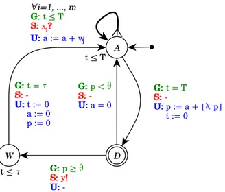
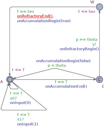
We present here a second approach aimed at overcoming the limitations of the asynchronous encoding introduced above. It handles input spike co-occurrence, and time-dependent potential decay, even if no spike is received. The neuron is conceived as a synchronous and stateful machine that: (i) accumulates po-tential whenever it receives input spikes within a given accumulation period, (ii) if the accumulated potential is greater than the threshold, the neuron emits an output spike, (iii) it waits for refractory period, (iv) and resets to initial state. We assume that no two input spikes on the same synapse can be received within the same accumulation period (i.e., the accumulation period is shorter than the minimum refractory period of the input neurons).

Definition 3.2 (Synchronous encoding). Let N = (θ, λ, p, τ, y) be a

leaky-integrate-and-fire neuron, let m be the number of ingoing synapses of N , let w1, . . . , wm be the weights of such synapses, and let T ∈ N+be the duration

of the accumulation period, then the synchronous encoding of N ,_{JN K}syn, into

timed automata is a tuple (L, A, X, Inv , Σ, Arcs), where: • L = {A, D, W} with D committed,

• X = {t},

Figure 3.2: Synchronous encoding of a leaky-integrate-and-fire neuron into a timed automaton. The (A → A) loop is actually a parametric and synthetic way to represent m edges, one for each input synapse.

• Σ = {y} ∪ {xi | i = 1, . . . , m},

• Arcs = {(A, t ≤ T, xi?, {a := a + wi}, A) | ∀i = 1, . . . , m} ∪ {(A, t =

T, ε, {p := a + bλ · pc, t := 0}, D), (D, p < θ, ε, {a := 0}, A), (D, p ≥ θ, y!, {}, W), (W, t = τ, ε, {t := 0, p := 0, a := 0}, A)}

where p, a and all wiare integer variables.

Such an encoding is represented in figure 3.2 and an intuition of its behav-ior is described in the following. It depends on the following channels, variables and clocks:

• t, xi, y and p are, respectively, a clock, the i-th input broadcast channel,

the output broadcast channel and the current potential variable, as for the asynchronous encoding,

• a ∈ N is a variable holding the weighted sum of input spikes occurred within the current accumulation period. It is 0 at the beginning of each period.

Locations are named as for the asynchronous encoding, but here they are subject to different rules:

3.1. LI&F NEURONS AS TIMED AUTOMATA 33 • The neuron keeps waiting in state A for input spikes while t 6 T and

whenever it receives a spike on input xi it updates a as follows:

a := a + wi

• When t = T the neuron moves to state D, resetting t and updating p as follows:

p := a + bλ · pc

• Since state D is committed, it does not allow time to progress, so, from this state, the neuron can move back to A resetting a if p < θ, or it can move to W, firing an output spike, otherwise.

• The neuron will remain in state W for τ time units and then it will move back to state A resetting a, p and t.

The innovation here is the concept of accumulation period. According to the asynchronous encoding, two inputs cannot occur into the same instant and, above all, their relative order is the only thing that influences the neuron potential: two consecutive input spikes would have the same effect regardless of their time difference. Thanks to the accumulation period of the synchronous encoding, the time distance between two consecutive spikes can be valorized: since the firing of transition (A → D), namely “the end of the accumulation period”, is not governed by input spikes as for its asynchronous counterpart but only by time, the neuron potential actually decays as time progress, if no input is received.

Note that, if the assumption requiring one input not to emit more than once within the same accumulation period does not hold (i.e. inputs frequencies are too high), the neuron potential would increase as if the two spikes were from different synapses.

Finally, it may be noticed that, as for the asynchronous model, a minimal automaton can be obtained by removing state D and adding more edges.

3.2

Spiking neural networks as timed automata

networks

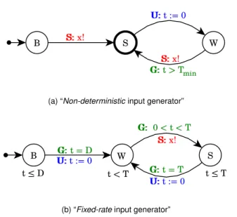
After showing how a timed automaton can encode a neuron, the main concern is about neuron interconnection, i.e., encoding leaky-integrate-and-fire spiking neural networks into timed automata networks by means of a proper channel sharing convention. Another relevant matter covered by this section is about inputs and outputs handling, for a given network. The input neurons of a net-work are encoded into input generators, i.e., automata emitting spikes over a specific output channel. We say that such generators feed the network, by producing input spikes for its neurons. Analogously, the spikes produced by any output neuron of a network are consumed by an output consumer. We say that such automata consume the outcome of the network, by receiving — and possibly inspecting — the output spikes produced by its output neurons. We also define a language for input sequences specification and show how to encode any word from such a language into a timed automaton able to emit it. Then we introduce non-deterministic input generators which are useful in those contexts where random input sequences are needed. Finally, we show how output consumers can be used to inspect, e.g., a neuron spike frequency. Let S = (V, A, W ) be a leaky-integrate-and-fire spiking neural network with V = Vi∪ Vint∪ Vo(as remarked in definition 2.1, we distinguish between

input, intermediary and output neurons), then the encoding of S into a timed automata network is given by the parallel composition of the encodings of all the neurons within the network:

JS K = ( n g∈Vi JgK) k ( n v∈Vint JvK) k ( n n∈Vout JnK k On)

where On are output consumers: the network has |Vout| automata of such a

sort.

The topology of network S, expressed in A, must be reflected by the way channels are shared between the automata encoding the neurons in S. So, let Σ = {yv | v ∈ V } be the set of broadcast channels containing the output

channel of each neuron composing the network, let inputs : V → Σ∗ be the function mapping each neuron v to the tuple of channels used by _{JvK for}

3.2. SNNS AS TIMED AUTOMATA NETWORKS 35 receiving spikes, let weights : V → Z∗ be the function mapping each neuron v to the tuple of weights used by_{JvK, and let output : V} → Σ be the function mapping each neuron v to the channel used by_{JvK for sending output spikes.} Then we impose the following constraints to_{JS K:}

• output(v) = yv, ∀v ∈ V ,

• inputs(v) = {yv | ∀(u, v) ∈ A}, ∀v ∈ Vint∪ Vo,

• weights(v) = {W (u, v) | ∀(u, v) ∈ A)}, ∀v ∈ Vint∪ Vo,

• for each v ∈ Vo, the output channel yv of v is the input channel of an

output consumer O.

In the rest of this thesis we may adopt the following notation to repre-sent the interconnection of automata. Let I1, I2, . . . be input generators, let

N , N1, N2, . . . be some neurons encoding, and let O be an output consumer,

then we may write: • (I1, . . . , In)

x

k N , where x = (x1, . . . , xn), meaning that each channel

xi is shared between Ii and N , carrying input spikes from the former to

the latter; • (N1, . . . , Nn)

y

k N , where y = (y1, . . . , yn), meaning that each channel

yi is shared between Ni and N , carrying the output spikes of Ni which

are received by N ; • N

y

k O, meaning that y is a shared channel carrying the output spikes produce by N and consumed by O.

3.2.1

Handling networks inputs

Here we discuss about the inputs used to feed spiking neural network. Es-sentially, neurons consume sequences of spikes. We propose a the grammar of a language over spikes and pauses defining how any valid input sequence may be structured. We also provide an encoding into input generators for such sequences, i.e., timed automata able to reproduce a given word over the proposed language.

Regular input sequences. Essentially, input sequences are lists of spikes and pauses. Spikes are instantaneous while pauses have a non-null duration. Sequences can be empty, finite of infinite. After each spike there must be a pause except when the spike is the last event of a finite sequence, i.e., there exists no sequence having two consecutive spikes. Infinite sequences are composed by two parts: a finite and arbitrary prologue and an infinite and periodic part whose period is composed by a finite sub-sequence of spike– pause couples which is repeated infinitely often.

Definition 3.3 (Input sequence grammar). Let s, p, ] and [ be terminal

sym-bols, let I, N , P1, . . . , Pnand P be non-terminals and let x1, . . . , xn∈ N+ be

some durations (that are terminals) then: IS ::= Φ s | P Φ s | Φ Ωω _{| P Φ Ω}ω Φ ::= ε | s P Φ Ω ::= (s P1) · · · (s Pn) P ::= p[N ] Pi ::= p[xi]

represents the ω-regular expression for valid input sequences.

The language L(IS) of words generated by such a grammar is the set of valid input sequences.

In definition 3.3, the symbol s represents a spike, p is a symbol represent-ing a pause, and each pause is associated to a natural-valued duration, as one can notice by the productions of P and Pi. The notation p[N ] represents

a pause whose duration is some number matching N , the regular expression for natural numbers, while p[xi] represents a pause whose duration is a given

number xi. This is important because pauses within the periodic part Ω, which

is repeated infinitely often, must be the same in all repetitions. Notice that any pause within any valid input sequence is followed by a spike.

It is possible to generate a generator automaton for any regular input se-quence, according to the following encoding.

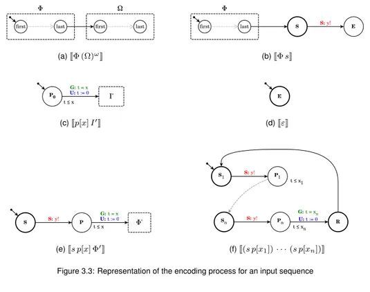
Definition 3.4 (Input generator). Let I ∈ L(IS) be a valid input sequence, let

3.2. SNNS AS TIMED AUTOMATA NETWORKS 37 timed automaton is a tuple_{JI K = (L(I ), f irst(I ), {t}, {y}, Arcs(I ), I nv(I )),} inductively defined as follows:

• if I := Φ (Ω)ω

– L(I) = L(Φ) ∪ L(Ω)

– f irst(I) = f irst(Φ), last(I) = last(Ω)

– Arcs(I) = Arcs(Φ) ∪ Arcs(Ω) ∪ {(last(Φ), true, ε, {}, f irst(Ω))} – Inv (I) = Inv (Φ) ∪ Inv (Φ)

• if I := Φ s

– L(I) = L(Φ) ∪ {S, E}, where S is urgent – f irst(I) = f irst(Φ), last(I) = E

– Arcs(I) = Arcs(Φ)∪{(last(Φ), true, ε, {}, S), (S, true, y!, {}, E)} – Inv (I) = Inv (Φ)

• if I := p[x] I0_{, with I}0 _{:= Φ (Ω)}ω _{or I}0

:= Φ s and x ∈ N+

– L(I) = {P0} ∪ L(I0),

– f irst(I) = P0, last(I) = last(I0)

– Arcs(I) = Arcs(Φ1) ∪ {(P0, t ≤ x, ε, {t := 0}, f irst(I0))}

– Inv (I) = {P0 7→ (t ≤ x)} ∪ Inv (I0)

• if Φ := ε

– L(Φ) = {E}, where E is urgent – f irst(Φ) = last(Φ) = E

– Arcs(Φ) = Inv (Φ) = ∅

• if Φ := s p[x] Φ0

with x ∈ N+

– L(Φ) = {S, P} ∪ L(Φ0)

(a)JΦ (Ω) ω K (b)JΦ sK (c)Jp[x] I 0 K (d)JεK (e)Js p[x] Φ 0 K (f)J(s p[x1]) · · · (s p[xn])K

Figure 3.3: Representation of the encoding process for an input sequence

– Arcs(Φ) = {(S, true, y!, {}, P), (P, t = x, ε, {t := 0}, f irst(Φ0))}∪ Arcs(Φ0)

– Inv (Φ) = {P 7→ t ≤ x} ∪ Inv (Φ0) • if Ω := (s p[x1]) · · · (s p[xn]) with xi ∈ N+

– L(Ω) = {S1, P1, . . . , Sn, Pn, R}, where R and all Siare urgent

– f irst(Ω) = S1, last(Ω) = R

– Arcs(Ω) = {(Si, true, y!, {}, Pi), (Pi, t = xi, ε, {t := 0}, Si+1) |

i = 1, . . . , (n−1)}∪{(Sn, true, y!, {}, Pn), (Pn, t = xn, ε, {t :=

0}, R)} ∪ {(R, true, ε, {}, S1)} ∪ {(R, true, ε, {}, S1)}

– Inv (Ω) = {Pi 7→ (t ≤ xi) | ∀i = 1, . . . , n}

Figure 3.3 depicts the shape of input generators. Fig. 3.3a shows the generator_{JI K obtained from an infinite sequence I := Φ (Ω)}ω: an unlabeled edge connects the last location of the finite prefix Φ to the first location of the periodic part Ω. In case of a finite sequence I := Φ s, as shown in fig. 3.3b, the last location of finite prefix Φ is connected to an urgent location S having an