Investigations of ferromagnet-organic bilayers for application in spintronics

Alma Mater Studiorum

_·

Universit`

a di Bologna

Scuola di Scienze

Dipartimento di Fisica e Astronomia Corso di Laurea Magistrale in Fisica

Investigations of ferromagnet-organic

bilayers for application in spintronics

Relatore:

Prof. Samuele Sanna

Correlatore:

Dott.ssa Ilaria Bergenti

Presentata da:

Mattia Benini

3

ABSTRACT

La fine degli anni 80 hanno visto la nascita della spintronica, una branca dell’elettronica che sfrutta, oltre che la carica, lo spin dell’elettrone. Questo campo di ricerca si è sviluppato grazie ad alcuni lavori pionieristici sulla magnetoresistenza in multistrati metallici ad opera di Albert Fert[1] (1988) e Peter Grünberg[2] (1989), lavori cha hanno valso a questi ricercatori il Premio Nobel per la fisica nel 2008. Il dispositivo spintronico modello, chiamato spin valve, è costituito da strati ferromagnetici disaccoppiati tra loro attraverso un materiale non magnetico di diversa natura (metallo o isolante). La resistenza di questo dispositivo dipende dall’ orientazione relativa della magnetizzazione dei due strati ferromagnetici. Più recentemente il campo della spintronica si è orientato verso l’uso di semiconduttori organici come materiale di separazione tra strati magnetici dando origine alla cosiddetta “organic spintronics”. In particolare, l’uso di semiconduttori organici permette di minimizzare i meccanismi di scattering di spin grazie al basso accoppiamento spin-orbita e interazione iperfine. Dopo i primi successi di integrazione di materiali organici in dispositivi spintronici, sono emerse alcune peculiarità dei comportamenti magnetoresistivi[3, 4] che indicano come le molecole giochino un ruolo maggiore rispetto al mero trasporto di correnti spin-polarizzate. In particolare, si sono evidenziate una serie di modifiche delle proprietà elettriche e magnetiche all’ interfaccia tra un materiale ferromagnetico e uno strato di molecole che possono avere effetti macroscopici sul funzionamento dei dispositivi[5-7]. Questo concetto è stato associato al termine spinterface. Questo nuovo tipo di interfacce è di notevole interesse in molteplici campi oltre la spintronica, come l’optoelettronica o le memorie magnetiche.

In questo lavoro di tesi si sono studiate proprietà magnetiche di bistrati cobalto/fullerene e cobalto/gallio-quinolina, con l’obiettivo di verificare il ruolo del materiale organico nella definizione delle proprietà magnetiche dello strato di cobalto.

Nel primo capito introdurrò brevemente alcuni concetti chiave della spintronica, soffermandomi sulla nozione di spinterface e sui risultati presenti in letteratura in tale ambito Nel secondo capitolo descriverò le proprietà ferromagnetiche rilevanti per il comportamento magnetico dei bistrati, come i vari contributi di anisotropia magnetica, i domini magnetici e il modello di Stoner Wohlfarth per la descrizione del processo di magnetizzazione di un materiale ferromagnetico.

Nel terzo capitolo descriverò gli apparati strumentali utilizzati in questo lavoro: la camera di deposizione per la crescita dei bilayer, il microscopio a forza atomica per le indagini morfologiche delle superfici di cobalto e il magnetometro MOKE (Magneto-Optic Kerr Effect) per lo studio del comportamento magnetico dei bilayer.

Nel quarto capitolo sono riportati i dati sperimentali e la loro discussione, con particolare enfasi riguardo lo studio delle proprietà magnetiche, con l’obiettivo di verificare la presenza di effetti di “spinterface”.

5

CONTENTS

1 ORGANIC SPINTRONICS AND SPINTERFACE ... 7

1.1 SPINTRONICS ... 7

1.1.1 SPIN VALVE AND GIANT MAGNETORESISTANCE ... 8

1.2 ORGANIC SPINTRONICS ... 10

1.3 THE SPINTERFACE ... 12

1.3.1 THE MOLECULAR SIDE ... 13

1.3.2 THE FERROMAGNETIC SIDE ... 14

1.3.3 EXPLOITATION OF THE SPINTERFACE PROPERTIES ... 14

1.4 MATERIAL OF INTERESTS ... 15

2 FERROMAGNETISM IN THIN FILMS ... 17

2.1 INTRODUCTION TO FERROMAGNETISM ... 17

2.2 MICROSCOPIC ORIGIN OF FERROMAGNETISM ... 19

2.3 ANISOTROPY ... 19

2.3.1 MAGNETOCRYSTALLINE ANISTROPY ... 20

2.3.2 SHAPE ANISOTROPY ... 23

2.3.3 SURFACE ANISOTROPY ... 25

2.3.4 STRAIN ANISOTROPY ... 25

2.4 DOMAINS AND THE STONER WOLFHART MODEL ... 26

2.4.1 MAGNETIC DOMAINS ... 26

2.4.2 THE STONER-WOHLFARTH MODEL ... 27

2.5 MAGNETIC ANISOTROPY OF ULTRA-THIN FILMS ... 29

3 EXPERIMENTAL SETUP ... 31

3.1 DEPOSITION APPARATUS ... 31

3.1.1 ELECTRON BEAM EVAPORATION ... 32

3.1.2 KNUDSEN CELL ... 33

3.2 MORPHOLOGICAL CHARACTHERIZATION BY ATOMIC FORCE MICROSCOPY ... 34 3.3 MAGNETIC CHARACTERIZATION BY MAGNETO-OPTIC KERR EFFECT

6

4 RESULTS AND DISCUSSION ... 41

4.1 COBALT THIN FILMS ... 41

4.1.1 SURFACE MORPHOLOGIES ... 43

4.1.2 MOKE MEASUREMENTS ... 48

4.2 BILAYERS Gaq3/Co AND C60/Co ... 53

4.2.1 MOKE MEASUREMENTS ... 54

4.3 POSSIBLE HINTS OF A SPINTERFACE FORMATION ... 58

5 CONCLUSIONS ... 63

6 SUPPLEMENTARY INFORMATION ... 65

6.1 PRINCIPAL UNITS IN MAGNETISM ... 65

6.2 THE HEISENBERG HAMILTONIAN ... 65

6.3 ERROR ANALYSIS FOR MOKE MEASUREMENTS ... 67

6.4 DETERMINATION OF THE MEDIUM GRAIN SIZE ... 68

7

Chapter 1

1

ORGANIC SPINTRONICS AND SPINTERFACE

The spinterface is a relatively novel word, introduced for the first time in 2010 by Stefano Sanvito [7] to name an interface between a ferromagnetic material and an organic semiconductor (OSC) layer featuring a strong hybridization. OSC molecules were first used for spintronic application in 2002 [7], as alternative materials to inorganic ones in magnetic tunnel junction [5] or in spin-valves fabrication. Initially chosen for their intrinsically weak spin relaxation mechanisms [5] it became clear that spintronic devices based on hybrid interfaces present peculiar functionalities, whose behavior was intimately due to the nature of interfacial layers [8].

In the following chapter a brief introduction to spintronic concepts is given, including a description of the spin valve and of the magnetic tunnel junction devices. Subsequently I will present the peculiar properties of spinterfaces with some examples to highlight the motivation of this work.

1.1

SPINTRONICS

The spintronics (shorthand for spin electronics) is a branch of “electronics” that exploits the carrier’s spin state to storage and process binary information.

Ferromagnetic metals have a spin-dependent density of states, when magnetized. At the Fermi energy there will be a spin-polarized electronic unbalance. This can be parametrized using the ratio of the difference between the two DOS over the overall DOS, both calculated at the Fermi energy:

� = ↑_↑ E_EF − ↓ EF

F + ↓ EF

(1.1.1)

Supposing a charge flow from such a spin-asymmetric material into a non-magnetic material, the current will be spin-polarized over a distance lower than the so-called spin diffusion

length _s . This because electrons injected into the non-magnetic material will be subject to spin scattering events. The value of _s depends on the specific properties of the non-magnetic materials [9]: _s is generally few nanometers in metals and it could reach hundreds of nm in non-doped semiconductors like Ge [10].

8

1.1.1

SPIN VALVE AND GIANT MAGNETORESISTANCE

The spin valve is the simplest spintronic device: it’s composed by two ferromagnetic layers decoupled by a non-magnetic spacer of width ≲ _s , as reported in Figure 1. Depending on the mutual orientation of the magnetization in the two ferromagnetic layers, the resistance of the device in the parallel state (both magnetizations are parallel to each other) has a lower resistance than the antiparallel state (the two magnetizations are antiparallel). The two configurations can show a relative change of resistance, even larger than 100% [9]. This effect is known as giant magnetoresistance (GMR) and it has been observed with different spacer materials [9].

Figure 1. Sketch of a spin valve.

The effect can be measured quantitively by the magnetoresistance ratio ∆ ⁄ , defined as the ratio of the difference between the resistance in parallel/antiparallel state and the resistance in zero applied field ( ,

∆

= ↑↑− ↑↓ (1.1.2)

The GMR depends on several factors, like the spacer thickness d, the material used for the device, and the temperature.

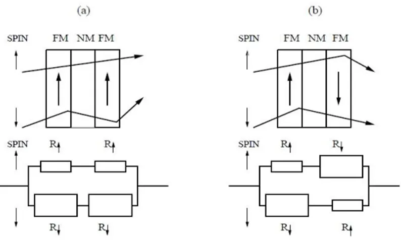
A simple model based on Mott’s two-current model of conduction was proposed to qualitatively explain the GMR in case of metal spacer [11]: the electrical conductivity is described by independent conducting channels, corresponding to the spin-up and spin-down electrons and considering different scattering rates of the spin-up and spin-down electrons. Following the Mott’s model, the spin valve can thus be modeled, as shown in Figure 2, as two couples of resistors connected in parallel; with larger resistance associated to scattering events of electrons with spin antiparallel to the magnetization. In the parallel state of the spin valve (a), electrons with spin-up are weakly scattered both in the first and second ferromagnet, whereas the spin-down electrons are strongly scattered in both ferromagnetic layers. Since the up- and down-spin channels are connected in parallel, the total resistance of the trilayer in its parallel configuration is mostly due to the low-resistance spin channel dominating the high-resistance of spin-down one.

9 Figure 2. Resistor model of a spin valve.

Thus, the total resistance of the trilayer in its parallel configuration is low. On the other hand, spin-down electrons in the antiparallel state (b) are strongly scattered in the first ferromagnetic layer but weakly in the second; for spin-up electrons the viceversa holds. This is modeled by one large and one small resistor in each spin channel. The two channels now have the same resistance, so the antiparallel configuration has a total resistance much higher than the parallel configuration.

The spin valve can be realized also using an ultra-thin insulator layer as spacer: in this case it’s called Magnetic tunnel junction (MTJ). The mechanism of magnetoresistance relies on quantum mechanical tunneling of the carriers. In such case the magnetoresistance (properly

tunneling magnetoresistance, TMR) is described by the Jullière model [12]. The tunneling current for each spin direction is proportional to the product of the density of states at Fermi level in the electrodes on both sides of the tunnel barrier:

= _{− � �}� � (1.1.3)

10 Following this model, the largest magnetoresistance is expected for electrode’s polarization close to 1. This specific case is obtained with metallic ferromagnets (HMF) A half-metal material is a ferromagnet that, due to the spin-split bands, possesses a Fermi energy that is in a bandgap for one of the two spin bands, while falling inside the other band, as depicted in Figure 3

1.2

ORGANIC SPINTRONICS

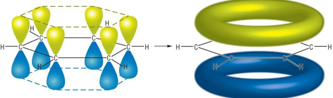
An organic material is primarily based on carbon and hydrogen -single molecules, short chains (oligomers) and polymers- and exhibits semiconducting properties. organic materials have quite different conduction mechanisms with respect to inorganic ones: in the case of small molecules the charge carriers are typically localized to single molecular orbitals, known as the highest occupied molecular orbital (HOMO) and lowest unoccupied molecular orbital (LUMO). Most of the organic solids are insulators, but when their constituent molecules have π-conjugate systems typically with benzene rings as the basic unit (Figure 4), charge carriers can move via π-electron overlaps, especially by hopping, tunneling and related mechanisms giving rise to a semiconducting behavior.

Figure 4. Left: carbons pi-conjugated 2p electrons of a benzene molecule. Right: their delocalization all over the molecule.

The use of organic semiconductors (OSC) as a spacer in spin valve has strongly emerged with the aim of extending the spin coherence length to tenths of nm to allow the spin manipulation. In fact, in OSC spin-relaxation mechanisms are intrinsically minimized by their nature. Spin–orbit coupling (SOC), proportional to the forth power of the atomic number Z, is very small because they are based on light elements like carbon, oxygen and hydrogen. Also, the hyperfine interaction is weak, because the transport properties are due to the delocalized electrons (π-conjugated) provided by carbon atoms: since they are p wavefunctions, they have no amplitude on the nucleus. Moreover, carbon atoms (the

11 backbone of the organic molecules) in their most abundant isotope (12C) have 0 nuclear magnetic moment.

Spin injection in OSCs was first demonstrated in a series of studies in the standard spin valve geometry [13, 14] with OSCs spacer approximately 100–200nm thick.

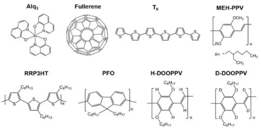
A large number of molecules (some of which are reported in Figure 5) has been successfully tested [15], like metal-quinolines (Alq3, Gaq3), fullerene (C60) and sexythiophene (T6).

Figure 5. List of some of the molecules used in organic spintronics.

The use of OSCs in tunneling devices has shown considerable achievements, namely, room temperature operation and very high MR values (up to 600%) at low temperatures [16, 17].

Figure 6. Up, left: Co/Alq3(2nm)LSMO MTJ device. Up, right: MTJ's positive magnetoresistance measured at 2 K. Down left: Co/Alq3(100nm)/LSMO spin-valve.

12 In experiments on spin valves including an organic spacer, negative magnetoresistance (lowest resistivity for antiparallel alignment of electrode magnetization) has been routinely found for some selected electrodes, namely La0.7Sr0.3MnO3 (LSMO) and Co. As reported in

Figure 6 (sources [4, 18, 19]) a negative magnetoresistance behavior is measured for a LSMO/Alq3(100nm)/Co spin-valve and is detectable even at room temperature.The same

Alq3 molecule in tunneling devices with same electrode configuration gave rise to positive magnetoresistance [18]. Considering the spin polarization sign of the ferromagnetic electrodes the different sign of MR in tunneling and transport regime could not be explained.A coherent picture invoking the role of molecular layers in tuning the spin polarization of ferromagnetic materials at the interface has been proposed [18] introducing then the concept of spinterface, and will be treated in the last section of this chapter. This discovery was of fundamental importance in the field of organic spintronics because it opens the door for a new class of spintronic devices, stemming from the concept of a new electrode whose behavior is determined by the interface [18].

1.3

THE SPINTERFACE

Energetics of molecular interfaces is a wide and complex topic, nevertheless it’s possible to highlight some important aspects. Molecules interact with surfaces with forces originating either from the “physical” Van der Waals interaction or from the “chemical” hybridization of their orbitals with those of the atoms of the substrate. Within a simple one-dimensional (1D) model, the only variable is the distance (d) of the adsorbing molecule from the substrate surface and the energy of the system is a function only of this variable i.e. = (see Figure 7).

Figure 7. Sketch of the differences in the 1D Lennard-Jones potentials for chemisorption (red line) and physisorption (blue line).

In case of an inert metallic surface, the interaction between them will be Van-der-Waals-like: the molecules is said physisorbed to the surface. The energy curve has shallow

13 minimum at a relatively large distance from the surface before the strong repulsive forces arising from electron density overlap cause a rapid increase in the total energy. In this case an investigation of the energetic structure of both the molecule and the metal involved shows no significant change due to the interaction. This can be the case with molecules such as gold [20]. If the metal is reactive to the molecule, then chemical bonds can be formed between them: the molecule is said chemisorbed to the surface. Energy curve is dominated by a much deeper energy minimum at shorter values of . Chemical bonds may be covalent or ionic in nature. Chemisorption involves a high energy of activation and it’s highly specific. The chemisorption is the case of interest for this work. In case of d metals like Co or Fe, it has been observed chemisorption of some specific molecular species, as it happens for cobalt/fullerene (Co/C60) [21] or cobalt/Al-quinoline (Co/Alq3) interfaces [22] The interaction produces various modifications of magnetic (or spin) properties on both side of the interface, as described in the following.

1.3.1

THE MOLECULAR SIDE

When the organic molecule chemisorbs over the ferromagnetic material’s surface, the energy levels of the molecule are modified, as depicted in Figure 8. The highest occupied molecular orbital (HOMO) and the lowest unoccupied molecular orbital (LUMO) are shifted in energy and broadened into a continuum due to the formation of chemical bonds between the molecular atoms and the metal surface’s atoms. Consequently, a broadening of the DOS of the energy levels occurs. More importantly, at least for spintronic applications, this broadening is spin-dependent: this is so because the broadening and shifting are driven by the individual coupling of each metallic state to the molecular state, and hence is related to the spin-dependent metal DOS [23]. This energy levels modification occurs mainly for the first molecular layer: the second organic layer would have a faint interaction with the ferromagnet’s atoms, resulting in a weak perturbation. The energy shifts can vary depending on the metal and the molecules forming the spinterface, depending on the type of molecular orbitals and metallic bands involved in the hybridization. This is remarkable since can be exploited to tailor the ferromagnetic behavior of one terminal of a spin valve.

Figure 8. Sketch of spin-dependent energy broadening of a molecular energy level due to the interaction with the metal surface. Taken from [7].

14

1.3.2

THE FERROMAGNETIC SIDE

The formation of a spinterface has significant effects even in the inorganic side, at least regarding its magnetic properties. The deposition of organic molecules over ferromagnetic thin films induces modification of its magnetic anisotropy. As a notable example, it has been found, both theoretically and experimentally [24], that the deposition of C60 over a 5.5-layer

cobalt has the effect of rotating its easy axis magnetization from being in-plane to

out-of-plane, making it perpendicular to the film plane after just a complete covering of one monolayer, as depicted in Figure 9. This effect is reported to be due to the bonds formed between the surface Co atoms and the C atoms of the fullerene: in particular, the 3d Co electrons and the delocalized p electrons of C60.

Figure 9. Reorientation of the easy axis of a cobalt thin film covered by one layer of fullerene.

It is also reported [25] that deposition of C60 over thin films (less than 3 nm) of copper

(diamagnetic) or manganese (paramagnetic) produces an emergent ferromagnetic state of both metals, provided that the film is grown in presence of a sufficient magnetic field. This is reported to be due to an exchange strength between interfacial atoms greater than the one possessed between metal atoms inside the film.

1.3.3 EXPLOITATION OF THE SPINTERFACE PROPERTIES

The spinterface formation opens a wide range of possibilities for spintronic applications. Considering the well-known spin valve geometry, the spin-dependent DOS possessed by OSC in contact with a ferromagnetic surface makes the spinterface an interesting electrode for spintronic devices, as it possesses and enhanced or inverted spin-polarization with respect to ferromagnetic electrode alone. An illustrative sketch is reported in Figure 10. The spin-dependent DOS of the organic layer can be modeled by a Lorentzian function [23]:

↑ ↓ _{= �} − Γ↑ ↓

15 where Γ↑ ↓ is the spin-dependent broadening of the molecule’s LUMO and ∆ ↑ ↓ is the spin-dependent distance between the effective molecular energy level and the metal’s Fermi energy. The spin polarization of the interface can be quantified by

� = ↑_↓ EF − ↓ EF EF + ↓ EF

(1.3.5)

Now, if Γ↑ ↓ ∆ ↑ ↓ (case b in Figure 10), then � > � , meaning that the spinterface has a spin-polarization greater than the sole ferromagnetic layer. Instead, if Γ↑ ↓ ∆ ↑ ↓ (case a in Figure 6), then � ≈ −� : this means that the formation of a spinterface results in a layer with spin-polarization inversed respect the sole ferromagnetic layer. This effect is known as spin filtering and is the explanation of the negative giant magnetoresistance measured in organic spin valves[8, 18, 26]. This is evidence that the magnetoresistance of a spin valve can be modified even by external stimulation of the organic side[5, 23].

The possibility to modify the magnetization anisotropy of a ferromagnet is exploitable for magnetic data storage. Production of magnetic thin films with out-of-plane magnetization would mean shrinking the dimension of magnetic information units, because it reduces interactions between neighboring magnetic bits.

Figure 10. Two different energy configurations of the spinterface. Taken from [23].

1.4

MATERIAL OF INTERESTS

For this work two molecules were chosen, gallium-quinoline and fullerene (C60).

Tris(8-hydroxyquinolato)gallium, or gallium-quinoline (Gaq3) is a coordination complex molecule, in which a gallium atom is bonded to three hydroxyquinoline ligands. (see Figure 11). Aluminum-quinoline were initially studied and carried out successful results as spin-filtering[27] effect and negative magnetoresistance.[4, 8, 18] It has been shown[28] that

16 choice of the coordination atom doesn’t affect the electronic and magnetic properties of [22] so spinterface effects are expected with Gaq3

Figure 11. Left: a gallium quinoline molecule. Right: Gaq3 molecule chemisorbed over a cobalt slab; molecule's structural deformations are visible. Adapted from [28]. The second molecule investigated is fullerene (or buckyballs), that is a spherical shaped 0D molecule composed of 60 sp2 _{hybridized carbon atoms (see Figure 12). Interfaces}

between C60 and a ferromagnetic thin films can show high spin-polarization[29], and

rotation of the magnetization easy axis has been reported for a cobalt ultra-thin film covered by fullerenes[24].

17

Chapter 2

2

FERROMAGNETISM IN THIN FILMS

In this chapter some important concepts in ferromagnetism will be described. After a short introduction of magnetism and ferromagnetism, the magnetic anisotropy will be introduced and discussed, along with the various types of anisotropy terms that a ferromagnetic material can possess, with a focus on the anisotropy of thin magnetic films.

2.1

INTRODUCTION TO FERROMAGNETISM

When discussing magnetism, it’s necessary to take care of system of units used. Magnetic fields generated by currents of any kind are denoted by H and are given in units of Ampère per meter

m in SI system, and in Oersted (Oe) in cgs system: dimensionally, it represents

a current flux. What is commonly called a magnetic field B should instead be called magnetic

induction; it’s measured in Tesla (T) in SI and Gauss (G) in cgs. B represents the total

magnetic field present in point in space. In free space, the difference between B and H is merely a constant, called the vacuum magnetic permeability = � ∙ − m If a physical system is present, then it will interact with the external field, producing a magnetic response in the form of a magnetic moment, whose volumetric density is called magnetization M and is given in

m in SI and Oe in cgs. Field B is then given by

� = � + γ � (2.1.1)

where is the and γ is a constant which account for different unit system[30] (see Supplementary). The SI system will be adopted in the throughout.

The magnetic response of the physical system is not unique and depends on its various characteristics. The material is said linear if the magnetization is proportional to the applied magnetic field,

� = χ� (2.1.2)

18 Equation (2.1.1) can now be written as

� = + χ � = � = � (2.1.3)

where is called the magnetic permeability. The material is then said diamagnetic if χ<1,

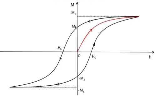
paramagnetic if χ>1. Not all the materials, anyway, have their magnetization proportional to the applied field. Among these, there are ferromagnetic materials, for which M is also a multivalued function of H and depends on the history of the applied field. A typical case is shown in Figure 13, which plots the component of M in the direction of H, as a function of the magnitude of H. Such a curve is called hysteresis loop. Starting with an unmagnetized ferromagnet, an external field of increasing magnitude H is applied long a certain direction; this produces a magnetization of the material, that grows up to a certain value called

saturation magnetization M . If the field then is reduced to zero and subsequently increased

in the opposite direction, M would then decrease to 0 and then increase in the field direction, reaching the value −M .

Figure 13. A hysteresis curve for a ferromagnet.

The peculiarity is that the magnetization curve doesn’t go back along the previous path; it rather decreases slower than the previous increase and has a non-zero value at H=0, called

residual magnetization M . It is necessary to reach a value −H , called coercive field, to

demagnetize the ferromagnet. Reversing the process, the behavior of M is symmetrical to the previous one: it increases to −M when = , goes to 0 when H = H and then saturates again to M .It is worth noticing that there is a whole continuum of hysteresis curve, each of which can be obtained by a proper choice of the maximum and minimum value of the applied field. The one depicted in Figure 13 is called limiting hysteresis curve, attained by applying a field of magnitude sufficient to saturate the magnetization of the ferromagnet; it encloses all the other possible loops.

19

2.2

MICROSCOPIC ORIGIN OF FERROMAGNETISM

The origin of ferromagnetism lies, quite remarkably, in the electron-electron interaction [30] what emerges from quantum mechanics (see Sec. 6.2) is that it’s possible to describe a ferromagnetic system composed by N interacting spins � subjected to an eventual external magnetic field B by the following Hamiltonian [31]

ℋ = ℋ + ℋ = − ∑ , � ∙ � , =

+ ∑ �

=

∙ � (2.2.4) where g is the so-called g-factor and is the Bohr magneton. The second term is the interaction between each magnetic moment and the external magnetic field, while the first term accounts for an interaction between two spins � , � , the strength of which is encoded in the exchange integral _, :

, = ∫ � � �∗ � � � |� − � |�∗ � � � (2.2.5)

Here, � is the wavefunction of the system that possesses the interacting spin. Such system could be a single electron as well as the valence electrons of an ion: this all depends on the material one is investigating. It is the value of J that determines the interaction behavior of the system; when > the energy term is negative, producing a parallel coupling of the spins; this produces the ferromagnetic behavior of the system. If < then the antiparallel coupling of the spins is preferred, and this produces an antiferromagnetic behavior. Here only the ferromagnetic case will be treated.

2.3

ANISOTROPY

Consider a ferromagnetic particle with magnetic moment �, that forms an angle with a fixed external magnetic field � (see Figure 14). Given that the interaction energy between the two is − Hcos , at thermal equilibrium the probability to have a particular angle at a temperature T is proportional to

[ Hcos_� ] = [ cos ] (2.3.6)

20 cos =∫ ∫ cos exp[ cosθ]sin �

� �

∫ ∫ exp[ cosθ]sin� � � = = coth − =

(2.3.7)

And is called the Langevin function. The quantity cos represents the component parallel to H of the normalized magnetization vector:

cos = M_{M = (}H _{� )}H (2.3.8) This equation classically describes the behavior of paramagnets; the magnetization goes down to 0 in the limit of a vanishing applied field. Ferromagnets do possess a non-zero magnetization below a critical temperature, or after a sufficiently large applied external field is turned off. Any ferromagnet thus needs to be described also by some other energy term that contains a dependence on the orientation of the sample with respect to the external field. Ferromagnetic materials, in fact, are not isotropic, and so not all the possible values of are equally probable; there are different kinds of anisotropy that can be possessed by the material, depending on the intrinsic properties of the constituents or external factors. In the following the most important anisotropies terms will be described.

Figure 14. A magnetic particle inside a magnetic field.

2.3.1

MAGNETOCRYSTALLINE ANISTROPY

It is caused by the electron spin-orbit interaction; since their orbits are influenced by the geometry of the crystal structure, so spins prefer to align along with well-defined crystallographic axes. Quantitatively the magnetocrystalline anisotropy energy term is small compared with the exchange interaction, but the direction of M is determined by this term (in absence of other anisotropy energy terms). Even if it’s possible to obtain the energy term starting from a quantum-mechanical framework, it’s standard to use phenomenological expression that are power series that take into account the crystal’s symmetries and with coefficients values obtained from experiments[30]. Typically, the volumetric energy density

21 is considered, and the expansion is made in power series of some function of the cosines of the angles formed between the crystalline axis and the magnetization (the projections of M)

ℰ = ∑ ∑

∞ =

(2.3.9)

The directions along which the sample is easily magnetizable are obtained by minimizing the energy term with respect to the directions.

To obtain the anisotropy energy, ℰ has to be integrated over the ferromagnet volume :

= ∫ ℰ

Ω � (2.3.10)

In the following the uniaxial and biaxial magnetocrystalline anisotropies will be described.

2.3.1.1 UNIAXIAL ANYSOTROPY

A crystal with uniaxial anisotropy is characterized by an axis along which the sample is easily magnetizable, and a plane perpendicular to it, along which the magnetization of the material is hard. There is only one parameter, the angle between the easy axis and the direction of M. A typical example is described in Figure 15, where the z-axis is defined as the easy axis for magnetization. The energy density term can be written as power expansion of the cosine of (representing the component of M parallel to the easy axis). This energy term is symmetrical with respect to the hard plane[30], so odd powers of the cosine of can be cancelled out. For any ferromagnet the 4-th order expansion is sufficient to describe the anisotropy[30], so

ℰ ≈ − + + = − + (2.3.11)

where is the z-component of the normalized magnetization vector, and are temperature-dependent constants. Crystals with a hexagonal close-packed structure as for example Co crystals possess this kind of anisotropy. There is only one parameter, the angle between the c-axis (0001) and the direction of M. The power series can be truncated to the first term if | | | |. It’s worth noting that what was previously called the easy axis may not really be the easy direction: this depends on the value of the constants. If < then it means that the c-axis is an easy axis: this is the case for Cobalt in his hcp phase: = ∙ ⁄ and = ∙ ⁄ [32]. whereas < implies that it’s a hard axis, and the ab plane is an easy plane of magnetization.

22 Figure 15. Uniaxial anisotropy.

2.3.1.2 BIAXIAL ANISOTROPY

The biaxial anisotropy is a typical characteristic of crystals with a cubic structure (bcc, fcc, sc). Defining the cartesian axis to lie along the crystallographic axis, the energy term is unchanged by permutations of the axis, so again odd powers of the cosine can be eliminated [30]. As shown in Figure 16 the frame of reference is chosen with the z-axis along the (001) direction. Let , , be the angles between � and the crystallographic axis, so that =

cos � � = , , : the energy density term is then

ℰ = + + + ( + + )

+ (2.3.12)

where , , are temperature-dependent coefficients taken from experiments. The first-order term is just a constant, so for energy changes consideration, it can be taken away, so

ℰ = ( + + ) + (2.3.13)

If > the easy axis lies along the (100) direction while the hard axis in the(111) direction: this is the case for iron, which has = . ∙ ⁄ and = ± . ∙ ⁄ [32]. On the contrary, if < the easy axis lies along the (111) direction while the hard axis in the (100) direction: this is the case for nickel, for which = − . ∙ ⁄ and = . ∙ ⁄ [32].

23 Figure 16. Biaxial anysotropy.

2.3.2

SHAPE ANISOTROPY

It’s possessed by every ferromagnets and depends entirely in its shape. to understand this, it’s useful to write down the Maxwell’s equation

� ∙ � = � ∙ � + � = (2.3.14) So

� ∙ � = −� ∙ � (2.3.15)

This implies that at the surface of the magnet the non-zero divergence of the magnetization vector results in the creation of a demagnetizing field � , that interacts with M. The energy associated with this interaction is called the magnetostatic interaction and is given by

= − ∫ � � ∙ � � �

Ω (2.3.16)

This energy term depends on the shape of the magnet: the easy axis of magnetization are the ones for which has a minimum. Evaluation of (2.3.) is not easy in general, due to the fact that the integrand is often not trivial: anyway, for some particular shapes it has a fairly simple calculation. Here are some examples, all regarding a polycrystalline ferromagnet: this ensures that the average magnetocrystalline anisotropy is zero. For an ellipsoid (see Figure 17), the demagnetizing field is uniform inside the body, so

� = −ℕ � (2.3.17)

24 Figure 17. An ellipsoid.

If the frame of reference is aligned with the ellipsoid’s semi-axis, ℕ it has a diagonal form[30]:

ℕ = ( ) � ℎ Tr ℕ = (2.3.18)

The energy is then

EM = V ℕ � ∙ � = V N M + N M + N M (2.3.19)

If the ellipsoid is a sphere all the three semi-axes are equal ( = = so there’s no preferred directions, so N = N = N = and E_M = −� VM . If two of the three semi-axes are equal in length (see Figure 18) then the ellipsoid is said prolate ( = < ) or

oblate ( = > ). It follows then that N = N > N for the prolate ellipsoid and N = N < N for the prolate. Equation (2.3.19) then becomes

25 EM = V[ M + M N + MzN ] = + V N − N Mz+ (2.3.20)

Constant term apart, the energy depends on the second power of the magnitude of the magnetization along the z-axis: this is exactly the same behavior found for a uniaxial magnetocrystalline anisotropy. This new uniaxial anisotropy term can be cast as

ℰ H= E_{V =}H M N − N cos θ + . = + cos θ (2.3.21)

The value of determines the easy magnetization’s direction of our sample. For a prolate ellipsoid N = N > N and the easy-axis lies along the z-axis; for a prolate ellipsoid N = N < N and the z-axis becomes a hard-axis.

A last but very useful example is the case of an infinite slab, that can be seen as the limit case , ⟶ ∞, ⟶ . In this case N = N = and N = [33], so

ℰ H= M cos (2.3.22)

It follows by a simple minimization than for an infinite slab, the normal to the surface is an hard axis while the plane is easily magnetizable.

2.3.3

SURFACE ANISOTROPY

It is caused by the behavior of the spins located at the surface of an isolated ferromagnet. On one side, they interact with the “internal” spins, whereas on the other side they have none of them: this means that the exchange interaction cannot be the same as in the bulk. This difference holds true even if the surface is an interface with another material, being it magnetic or not. From a phenomenological point of view the energy associated with this anisotropy should express a tendency of the spins to be either parallel or antiparallel to the surface. A possible first-order expression may be

= ∫ ∙

�Ω

(2.3.23)

where n is the unit vector perpendicular to the surface and a coefficient taken from experiments.

2.3.4

STRAIN ANISOTROPY

This type of anisotropy is caused by magnetostriction: if a ferromagnetic material has a magnetization M along a certain direction, then the material will experience an elongation or a contraction along that direction. The effect is quantified by the saturation magnetization =�, that is the ration between the body dilation over its original length, measured align

26 the direction of magnetization [34]. Values of are typically of order − − − and can be positive (dilation) or negative (contraction)[35]. There is an inverse effect, called the

Villari effect: an induced stress on the material induces a change in the magnetic anisotropy behavior, namely a modification of the easy-axis and, given that the material is already magnetized, an increase/decrease of the saturation magnetization. A simple mathematical expression can be used to quantify the density of energy associated to the action, in a fully

magnetized uniaxial ferromagnetic material, of a unidimensional mechanical stress of modulus � acting at an angle respect to Ms [32]

ℇ = − � = − (2.3.24)

This is another anisotropy term and depends in the product �: if its positive, then the stress direction becomes an easy axis; if its negative, it becomes a hard axis.

2.4

DOMAINS AND THE STONER WOLFHART MODEL

2.4.1

MAGNETIC DOMAINS

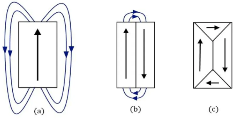
If all these energy terms are to be considered, the state with minimum energy is not trivial. If a magnetic material is in its ferromagnetic state (i.e. below the Curie temperature) and no external field is applied, the whole material may not exhibit a net magnetization. This is because the system may prefer to have a overall null magnetization, with the formation of a series of uniformly magnetized domains inside the sample. Domains form to minimize the overall free energy of the system, which accounts for anisotropic energy term, other than exchange energy. For example, domains are useful to reduce the demagnetizing field of the material. As an intuitive example, consider a rectangular-shaped magnet below the Curie temperature with no applied field H (see Figure 19); a state with a net magnetization M (a) implies the presence of a demagnetizing field that increases the magnetostatic energy. If energetically favorable, a state with domains (b, c in Figure 19) helps reducing the external demagnetizing fields.

Figure 19. A simple scheme to show how domains can reduce the demagnetizing field of a sample. Black lines: magnetization vectors. Blue lines, demagnetizing fields.

27 There are two common arrangements of two neighboring domains: either they have a 180° rotation of M or a 90° rotation. It’s clear that this rotation, albeit reducing the magnetostatic energy, increases the exchange energy along the domain wall, that is the surface that divides the two domains. It turns out that’s energetically preferred for domain formation to have a wall of a certain thickness , along which the magnetization gradually rotates; the value of ranges from tens to hundreds of nanometers [34]. There are two ways the magnetization can rotate in the wall: M rotates either in a plane parallel to the wall, then called a Bloch

wall, or in a plane perpendicular to the wall, then called a Néel wall (see Figure 20). From what’s been said, the condition for the formation of a domain structure to be formed is that the energy increase due to the domain walls formation is more than compensated from the magnetostatic energy reduction

Figure 20. Left: a Nèel wall. Right: a Bloch wall. Adapted from [32].

. This opens the possibility that ferromagnets with dimensions lower than a certain critical length presents a single-domain structure: the value of is roughly the same as [32]. For 3d ferromagnetic metals this length is within 100 nm [36].

2.4.2

THE STONER-WOHLFARTH MODEL

It’s one of the simplest, model that explains the hysteresis behavior of a ferromagnet. It assumes the magnet as a uniformly-magnetized, single-domain ellipsoid particle with uniaxial anisotropy. Suppose a field H is applied at an angle from the easy axis of the ferromagnet: it’s presence will rotate the magnetization vector M of an angle � from the easy axis (see Figure 21). The energy density is then

At fixed values of H and �, the direction of M is determined by energy minimization. �ℇ � = ; ( �ℇ � )�=� > (2.4.26) which yields [30] ℇ = sin � − − MHcos � (2.4.25)

28 Figure 21. A ferromagnetic particle feeling an external field H.

sin( � − ) + ℎ � � = (2.4.27)

cos � − + ℎ � > (2.4.28)

where ℎ =� MH

� . Equation (2.4.) admits an analytic solution only for two cases of . The

first case is = (i.e. H parallel to the easy axis). The minimization yields

ℎ + cos � sin � = � ℎ + ℎ cos � = (2.4.29) There are two possible solutions:

- a maximum for cos � = −ℎ (valid for |ℎ| < ; - a minimum for sin � = with + ℎ > .

The second solution implies that � = for ℎ > − and � = � for ℎ < . In the zone − < ℎ < both solutions are valid, but only one minimum is achievable elsewhere. From this we see that it’s important to know the field history: starting with a large positive field ℎ (see Figure 22) the only minimum possible is � = . This orientation won’t change until ℎ is lower than − , where the system is required to assume the other minimum, � = �: this means that the magnetization doesn’t change until a sufficiently large field is generated in the opposite direction, thus inducing an abrupt reorientation. In the interval − < ℎ < the system in the state � = has in a higher energy level than that with � = �, but can’t just jump into that state because there’s an energy barrier, that’s overcame when the applied field reaches a certain value. An analogous but specular reasoning is applicable in the opposite case, that is starting with a large negative value of ℎ and increasing it. The magnetization then rotates when the applied field has a value

29

H = H = _MK (2.4.30)

that is the coercive field. The second case is for = �, that is when H is perpendicular to the easy axis: this means that there is no anisotropy effect. The minimization procedure yields

ℎ − cos � sin � = � ℎ −cos � + ℎ cos � = (2.4.31) The results obtained are the same as the first case, but the case cos � = ℎ is now a minimum along with the cases � = , �. When − < ℎ < the magnet’s behavior is the same of a paramagnet with no hysteresis and zero coercive field For |ℎ| > the system goes into the solution � = or � = � depending on the sign of H. For all the other values of the equation for the minimum points has to be resolved numerically, but the behavior is similar to the case = (see see Figure 22): starting with a large positive value of h (that is, � = ) the magnetization gradually decreases (for decreasing h) to lower values of the magnetization’s component parallel to the field direction,M = M cos � , until this solution stops to be a minimum and starts to be a maximum. This happens for values of h that fulfills the requirement (2.4.); the system then jumps to the opposite branch, so the magnetization is reversed.

Figure 22. Hysteresis loops for the magnetic particle obtained for various choices of theta. Both the magnetization and the applied field are normalized by their maximum values.

Taken from [34].

2.5

MAGNETIC ANISOTROPY OF ULTRA-THIN FILMS

The case of relevance for this work is the magnetic anisotropy of ferromagnetic ultra-thin films (thickness less than 10 nm). It’s not possible to give a general description of such a system, because there are a lot of parameters that play a role: all types of anisotropies have to be considered.As a starting point, shape anisotropy is considered: the thin film can be modeled as an infinite slab, providing that the lateral dimensions are orders of magnitude

30 greater than the film thickness. Then, as showed before in Sec. 2.3.2 , the shape anisotropy term suggests that the magnetization lies inside the film’s plane. The contribution stemming from surface anisotropy is not trivial to obtain: it depends on the elements composing the ferromagnet film, the substrate’s chemical composition plus its magnetic behavior and the interaction with an eventual capping layer.

If there’s a lattice mismatch between the substrate’s surface cell and the ferromagnetic crystals cells then strain is inferred into the film while it grows, thus inducing a strain anisotropy. Film growth also affects the magnetocrystalline anisotropy: depending on deposition technique and substrate phase/morphology, the resulting thin film can be either polycrystalline or a single crystal: in the first case the magnetocrystalline anisotropy is expected to average out. If a single crystal is obtained, its easy axis direction depends on the phase possessed by the ferromagnetic crystal and its orientation relative to the film shape: these are determined by the growth condition and the selected substrate.

Some examples are illustrative. Polycrystalline nickel thin films in Au(111)/Ni/Au(111) structures are ferromagnetic for thicknesses greater than 5 Å, with an in-plane easy axis[37]. It has been shown that for ultra-thin Iron epitaxial films grown over a Pd(100) surface[38] the easy axis direction depends both on film thickness and deposition temperature : for = K the iron film has an easy-axis rotation from out-of-plane to in-plane for thicknesses greater than 2.5 ML, whereas for = K the magnetization is always

in-plane. Polycrystalline cobalt thin films in Au(111)/Co/Au(111) are always ferromagnetic, but the easy axis (uniaxial) rotates from out-of-plane to in-plane for thicknesses greater than 18 Å circa[37, 39]. On the other hand even a 1ML of cobalt deposited over Cu(100) presents an in plane easy axis [40].

31

Chapter 3

3

EXPERIMENTAL SETUP

The synthesis of heterostructures including a hybrid interface involves different deposition techniques. Moreover, high vacuum conditions have to be ensured to preserve the quality of interfaces and avoid oxidization and spurious contaminations. The deposition apparatus is then a complex system including UHV chambers devoted to different deposition techniques. In this chapter, the deposition techniques used for the synthesis of the analyzed bilayers will be described. Moreover, a brief description of the techniques used for their morphological and magnetic characterizations is presented.

3.1

DEPOSITION APPARATUS

The deposition system used for preparing the sample is schematized in Figure 23 and it consists of four different ultra-high-vacuum steel chambers connected with gates (G). Samples are inserted/extracted in the introduction chamber(IN), connected with a scroll pump(SCR) and a turbo pump (TP). This chamber is the only one exposed directly to the air during the sample loading, then its base pressure does not surpass the 10-7 mbar. The introduction chamber is connected with a second chamber devoted to the deposition of metals that we call metals chamber (MEC). It is equipped with a vertically displaceable sample-holder and a horizontally displaceable quartz crystal microbalance for deposition rate measurements. The metal’s source is a triple-gun electron beam evaporator; the vacuum is produced and kept by a turbo pump, allowing to reach pressures lower than ∙

− _{. A third chamber is devoted to the deposition of organic compounds and we call}

it organic chamber (ORC). It contains a vertically displaceable sample-holder and a fixed quartz crystal microbalance. Vacuum is provided by a cryo-pump ( − ). The organic molecules are evaporated from three different Knudsen cells. The forth chamber connecting the MEC and the ORC is the mask chamber (MAC). This chamber is equipped with a mask exchanger and allows the transfer of samples for deposition in the MEC and/or the ORC in UHV and clean conditions. Its base pressure is close to ∙ − . The sample can be displaced between the various chambers thanks to 4 fork-shaped arms (FA); two placed orthogonally placed in the inlet, two in the mask chamber. Pressures in the various chambers are measured by full range sensors, labeled by S in Figure 23 (Pirani and Cold Cathode).

32 Figure 23. Schematics of the deposition's apparatus.

3.1.1

ELECTRON BEAM EVAPORATION

The electron beam evaporator allows the sublimation of materials with high melting point, like metals. For this experiment, it was used for the evaporation of cobalt.

Electron beam evaporation technique involves heating a source of the desired material using electrons thermionically emitted from a tungsten wire. As the temperature of the source increases, the source starts evaporating the material; that is deposited over a suitable target substrate. The source heating is obtained by electron bombardment: electrons are produced by thermionic emission from filament of tungsten in which a large current is flowing. Thermoemitted electrons are then accelerated toward the source by high voltage. The source could have different form: in our case we used a Cobalt rod, alternatively a boat containing the material to be evaporated could be used.

The filament is made of tungsten doped with 1% thorium which function is to lower its work function and facilitate the thermoemission. The filament has the shape of a coil that surrounds the source; this configuration provides a uniform heating of the W filament. It is worth noticing that the rod (or the crucible) needs to be centered and perpendicular to the coil, and that should never be in contact to the filament to avoid shorts circuiting after the application of the High accelerating voltage; the evaporated material passes through a collimator to sharpen the flow, and then reaches the substrate when it starts to nucleate. To avoid overheating of the system, the electron gun is surrounded by a water-cooled copper shielding. The electron gun is connected to a controlling device able to tune:

- the current for the filament;

33 An additional flux monitor is included in the system for measuring the evaporating material’s flux. Another method for controlling the amount of evaporating material is by a direct measure of the electron current that exits the source (emission current). The emission flux can be adjusted by tuning three parameters, the emission current, the applied direct voltage between the filament and the source, and the z-position of the source. The density current of the thermionically emitted electrons is an exponential function,

= �exp [−_{� ]}� (3.1.1)

where W is the metal work function, k is the Boltzmann constant, A is a parameter specific of the filament and T is the temperature. Since the T is a function of the filament current, small variations of this parameter will in turn give strong variation of the emission density current and consequently of the evaporation rate. The voltage applied between the filament and the rod turns out to be a more accurate parameter with regards to the control of the evaporation rate, since the energy possessed by the electrons is a linear function of it. The relative position between the filament and the source is also an important parameter, especially if the source is a rod. To have an optimal evaporation the source needs to have its highest point exactly in the plane that contains the rod. If it were lower, the electrons available for the heating would be not enough; if it were higher, the evaporating material wouldn’t have a direct path towards the substrate, and the heating would produce a structural damage of the rod and consequently its collapse. Moreover, the deposition process needs to operate in high vacuum conditions (10-7-10-9 mbar):

- electrons travelling from the filament to the source are assured not to lose energy ionizing air molecules and producing sparks harmful to the device.;

- it avoids the presence of all kind of contaminants that otherwise would be deposited over the surfaces of the evaporator or the chamber;

- it ensures the evaporating molecules to have a mean free path sufficient enough to reach the substrate.

3.1.2

KNUDSEN CELL

A Knudsen cell is an evaporation cell designed for soft materials, like organic molecules. It’s designed expressly to produce an extremely uniform heating of the source.

In this experiment, two Knudsen cells were used, for evaporating the two organic molecules. A sketch of the device is reported in Figure 24.The powder of the desired material is put inside a quartz crucible, surrounded by a liquid metal that ensures thermal contact with a heat reservoir.

34 Figure 24. A Knudsen cell.

3.2

MORPHOLOGICAL CHARACTHERIZATION BY

ATOMIC FORCE MICROSCOPY

The atomic force microscope is a powerful instrument for surface morphological imaging with a resolution ranging from tens of micrometers down to tens of nanometers. Invented in 1986 by Gerd Binning and Calvin Quate[41] it’s one of the scanning probe microscopy instrument, is strength being the ability to scan non-conductive surfaces.

The instrument is basically a flexible cantilever with a nanometer-sized tip (with a certain shape) that gets placed in the proximity of the surface to analyze (102 to 10-1 nm depending on the technique used). The tip feels a force due to the interaction with the surface. The distortion induced in the cantilever is measurable, and from its measurement it’s possible to obtain the value of the tip/surface interaction.

The image is taken by scanning line by line a selected area of the surface: the tip scans forward and backward a line (fast scan), then moves up to the next one and starts again. In the end a NxN matrix is obtained, each element being a measure z((xi,yj)) of the interaction

in the point (xi,yj). The matrix in then rendered by a pc imaging software, as a 2D or 3D

image. The software used for data analysis is Gwyddion.

To qualitatively describe the interaction between the tip and the surface, a Lennard-Jones potential (Blue line in Figure 25) is used,

35 Figure 25. Range of application of various AFM techniques.

where = is the energy minimum; the first term in the square brackets represents a repulsive term while the second term represents an attractive term.

The cantilever is made typically in silicon, and the tip is obtained by photolithography technique or chemical etching. The cantilever curvature (induced by the interaction) goes from 1 nanometer to several tens of nanometers; it is measured in different ways as described in Figure 26. A laser beam is reflected into a photodiodes system, calibrated to have the laser spot in the center when no interaction occurs (the lever is not curved).

Figure 26. Sketch of the deflection measurement.

When a force (that has two components, parallel and normal to the plane containing the lever) acts over the tip, the induced curvature of the lever makes the laser spot deviate from the rest position. This deviation is measured as change in the collected intensity in the photodiodes and is converted in a measure of the force acting over the tip.

36 The tip of the AFM can have various interactions with the surface the most important ones being[42]:

• a dipolar Van der Waals interaction, when the tip is in the attractive zone of the potential ( < ;

• repulsive contact forces when > (ultimately due to Pauli repulsion); • electrostatic forces if local charges form for some reason over the surface; • capillarity forces that may arise ifthere’s moisture presence over the sample;

During scanning, the cantilever-tip system is moved over the surface thanks to a system of piezoelectric transducers, called scanner that ensures very precise displacements (precision of a fraction of an Ångstrom); their movements are controlled by the instruments electronic. In particular, a feedback system is implemented that keeps the tip/surface distance at the desired distance. The use of piezoelectric materials can induce artifacts in the measures, due to their intrinsic response to electric field like, nonlinear or hysteretic deformations; they can however be corrected with a certain effectiveness by dedicated software. The AFM has two main modes in which can be used. In what is commonly called the contact mode, the tip is placed in “contact” with the surface to analyze, so that the repulsion is balanced by the elastic force generated in the lever; the scan is made by keeping fixed (thanks to the feedback system) the interaction’s force or the tip/surface distance. This operation mode can0t be used over soft surfaces, because there would be the concrete risk of sample damaging. In the

non-contact mode, instead, the tip is placed at distances greater than and the lever is kept in oscillation (by a piezo transducer) with a certain frequency. Near the surface (in the attractive zone, see Figure 25), the tip feel’s the surface and the oscillation’s amplitude, phase and frequency are modified. This mode can be used for soft materials (like organic molecules) but the main disadvantage (respect to the non-contact) is a loss of resolution.

Whatever the mode the AFM is used, it’s of primary importance to shield it from external vibrations. For this issue, various anti-vibrations solutions are used. For the instrument used in this work, the AFM is placed over a base surjected by a spring, in a sealed steel chamber, posed over an anti-vibrating basement.

Over the years mathematical models for an equation of motion for a cantilever-tip in interaction with the surface has been developed and is still a field of research but goes beyond the scope of this work.

3.3

MAGNETIC CHARACTERIZATION BY

MAGNETO-OPTIC KERR EFFECT

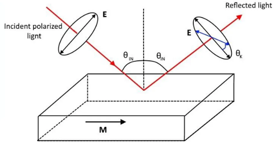
The MOKE, acronym for Magneto Optical Kerr Effect, is a magneto-optical phenomenon that is proper of ferromagnetic elements. When a beam of polarized light gets reflected by a magnetized surface, the reflected wave’s polarization vector ϵR is shifted by an angle

w.r.t the incident one, ϵI; this is caused by the presence of a magnetic field inside the material. This effect is explainable in a quantum mechanical framework as well as in a classical mechanical one. The former explains it in terms of the spin-orbit interaction between the

37 electrons spin and the orbit caused by the EM wave passing through the material; the latter makes use of Jones calculus.

The surface to be investigated (Figure 27) is shed by a beam of linearly polarized light (LLP), whose electric field Ei oscillates in the direction parallel to the plane of incidence (defined as the plane containing the incident ray and the reflected one). If a magnetic field H is acting in the reflecting material, the reflected light has its electric field Er rotated by an angle θK

that is given by

= _� (3.3.3)

where and are, respectively, the components of Er perpendicular and parallel to the plane of incidence.

There are three typical MOKE setup which can be implemented, each one depending on the direction of the applied field w.r.t. the plane of incidence and the magnetized film’s surface. In a polar configuration, H is perpendicular to the film’s surface, while in a transversal configuration is perpendicular to the plane of incidence. The last one, the longitudinal MOKE setup, has H inside both the film’s surface and the plane of incidence. This is the configuration implemented in this work and will be now described (see Figure 28).

Figure 27. Kerr rotation of a linearly polarized electromagnetic wave reflected by a magnetized surface.

A He-Ne laser (λ=632.8 nm) acts as the LLP source, and is placed over a first optical bench, aligned with a vertical polarizer(P1) and a beam splitter (BS). The former ensures that the incident light is fully linearly polarized w.r.t. the the incidence plane; the latter (made of amorphous glass to avoid undesired optical effects) is necessary for obtaining a reference signal. The BS reflects part of the light to a photodiode (D1), that collects the incident photons and produces a voltage signal. The not reflectedlight passes through a focusing lens

38 (L1) and collides with the surface sample (SS), with a small angle φ from the surface’s normal vector.

Figure 28. Schematics of a MOKE setup.

The reflected ray crosses a shutter (VF), a focusing lens (L2) a second polarizer (P2) and eventually it reaches a photodiode (D2), which collects it and produces a voltage output. All these three elements are kept aligned with each other and with the reflected ray by fixing them over a second optical bench, placed specular to the first one. The sample is placed on thetip of the sample holder (SH); it allows rotations around the surface’s normal direction, translation and/or rotation of the surface to guarantee the incoming beam to be reflected at the proper angle and position. The magnetic field H is generated by a couple of aligned electromagnets (EM), placed parallel to the surface so that the magnetization M is generated

inside both the surface and the plane of incidence. Each electromagnet is basically a coil, with a soft ferromagnet on top of it to produce a more homogeneous and focused field in the direction perpendicular to the coil. The second polarizer has its polarization axis � of an angle � ± (with “small”) w.r.t. the first polarizer’s � (Figure 29): this is meant to allow a small fraction of the unrotated light to reach the detector. The intensity measured by the photodiode is, for small ,

= | sin ± cos | ≈ | ± | (3.3.4) where the ± sign enters because the parallel component is inverted when the magnetization changes.This shows that if a part of the unreflected light (represented by ) hits the photodiode, the intensity measured becomes detectable ( can be four orders of magnitude greater than ) and sensible to the sign of the magnetization. All the setup is placed inside a box, that shields it from all external light sources. To avoid undesired external vibrations, an anti-vibration device is placed between the instruments and the support base. The data acquisition is operated by a PC program created with LabView. The computer receives the digital signal sent by an ADC that receives the voltage outputs from the two photodiodes; it also pilots the two electromagnets.

39 Figure 29. Schematic representation of polarization axis rotation.

41

Chapter 4

4

RESULTS AND DISCUSSION

In this chapter I will report the fundamental results obtained in my work. I’ll first describe the synthesis and the morphological and magnetic characterization of Cobalt thin films. Then I will investigate the properties of bilayers including Cobalt and OSC evidencing their peculiar properties with respect to the sole Co layer.

4.1

COBALT THIN FILMS

A series of Cobalt thin films with various thicknesses were deposited by e-gun on single crystal substrates. All samples were deposited at Room Temperature (RT), in high-vacuum conditions on pre-cleaned substrates. The considered substrates were:

- MgO (111) provided by MaTeck GmbH; - Al2O3(0001) provided by Crystal GmbH.

We expect that RT high-vacuum deposition of Co gives rise to single phase fcc Co on MgO (111) and hcp Co on Al2O3(0001).

Substrates were cleaned following this procedure:

- 4 cycles of 10 minutes RT ultrasonication bath in acetone (Normapur 99.999%); - 1 cycle of 10 minutes RT ultrasonication bath in acetone (Sigma Aldrich 99.999%); They were then mounted on the sample holder, introduced in the UHV chamber; subsequently they were annealed at a pressure of ⋅ − mbar for 30 minutes at 260°C, to help the desorption of organic contaminants and water. After annealing, without breaking the vacuum to preserve the interfacial quality, cobalt has been deposited by electron beam evaporation in high-vacuum condition (pressures of order − ). Deposition parameters are reported in Table 1.

The cobalt films thickness was measured by use of a TEM grid placed over one edge of the MgO surface (see Figure 30). After the cobalt growth, the zone resulted in a series of cobalt stripes divided by zones free of cobalt. An AFM imaging was made to measure the height of the cobalt stripe. Morphology of the cobalt samples was studied by AFM imaging. Grain mean diameter and surface roughness were obtained by the analysis of the AFM images. For details, see Supplementary information.

42

Co8 Co6 Co5 Co5A Co4

Substrate MgO(111) MgO(111) MgO(111) Al2O3(0001) MgO(111)

Pressure (mbar) < . ∙ − < . ∙ − . ∙ − . ∙ − . ∙ − Filament current (A) Applied voltage (V) Emission current (mA) . . . . . Flux current (nA) Rate (Å/s) _{. . . . .} Distance source-substrate (mm) . . . . . Co thickness (nm) . ± . . ± . . ± . . ± . . ± . Table 1. Deposition's parameters for the Co samples.

Figure 30. Sketch of the Co/MgO(111) samples obtained.

Preliminary X ray diffraction data (shown in Figure 31) indicate that films grown on MgO(111) are polycrystalline with both hcp and fcc phases. Films grown on Al2O3 presents

43 Figure 31. XRD measurements for Co5 (left) and Co5A (right) samples.

4.1.1

SURFACE MORPHOLOGIES

4.1.1.1 MgO(111) SUBSTRATE

An AFM image of m lateral size is reported in Figure 32. The surface was scanned before the cleaning process, to investigate the presence of contamination. They are clearly visible as bright spherical dots or ellipsoidal dots (as the one in the down-left corner). Also visible is the presence of scratches due to the substrate polishing and flattening processes.

Figure 32. MgO(111) surface.

To remove the contaminants, samples were washed in acetone (Sigma Alrich 99.8%)in ultrasonic bath for 10min for 3 times, then in isopropanol (Sigma Alrich spectroscopic grade 99.999%). This process allows to remove most of the surface’s organic contaminants and water.

44 4.1.1.2 Co8

A sample area of m lateral size is reported in Figure 33. The surface appears homogeneous but still there is presence of MgO(111) features (linear defect). Images show the presence of some defects ( bright spots) probably related to the growth process of Co layer and not to the substrates morphology.

Figure 33. Morphology of a 10x10 micrometer area of Co8.

An AFM image of nm lateral size is reported in Figure 34. This image is obtained by zooming the large-scale image. Cobalt grains with an average diameter of ± nm are visible, mostly with a spherical shape. The film is extremely flat with a surface roughness of . ± . nm, that is close to the fcc Co lattice parameters, . nm. It is also visible from the two profiles extracted (Figure 35), where the altitude differences are of the same order.