A new approach for the choice of motor and transmission in mechatronic applications

(1)

POLITECNICO DI MILANO

Facoltà di Ingegneria Industriale

Master of Science in

Mechanical Engineering

A NEW APPROACH FOR THE CHOICE OF

MOTOR AND TRANSMISSION IN

MECHATRONIC APPLICATIONS

Supervisor : Prof. Giancarlo Cusimano

MSc Thesis of: Xiangyi Peng ID. 780169

(2)

Index

Abstract ... 4

Introduction ... 5

Chapter 1 :Introduction to the conventional approach... 7

1.1 Scheme of the Drive System ... 7

1.2 Motor Characteristics ... 8

1.3 Constraint Inequalities During Work ... 9

1.3.1 Speed Limit ... 9

1.3.2 Continuous Duty Limits... 10

1.3.3 Dynamic Limit ... 15

1.3.4 Conclusion of the Constraint Inequalities ... 15

1.4 Transmission Characteristics ... 16

1.5 Load Specification ... 17

1.6 Feasibility Criterion ... 17

Chapter 2: Losses in Brushless Motors... 19

2.1 External Joule Losses... 20

2.2 Hysteresis Loss ... 21

2.3 Eddy Current Loss ... 24

2.4 Mechanical Losses ... 26

2.5 Testing... 27

2.5.1 Resistance Testing... 28

2.5.2 EMF Testing ... 29

2.5.3 Torque Testing ... 30

Chapter 3: New Approach... 33

3.1 Performance Curve of the Motor ... 33

3.2 Torque Limit and Inequalities... 34

3.3 Solution of the Parameters ... 35

3.3.1 Solution of 𝑀_𝑙𝑖𝑚 ... 35

3.3.2 Solution of 𝑀_ℎ, 𝑟_𝑒 and 𝑤... 36

3.4 Representation in the Plane 𝜔_𝑚 − 𝑀_𝑚... 37

3.5 Load Representative Point ... 38

3.6 Effect of the Transmission Ratio ... 39

(3)

Acknowledgements ... 53

Appendix A ... 54

Appendix B ... 55

Appendix C ... 56

Main MATLAB code of the model in MATLAB R2009b ... 56

subprograms to calculate load acceleration, velocity and position ... 60

(4)

Abstract

The main objective of the paper is to present a model for choosing proper motor and transmission under predicted periodic load taking into account the iron losses and mechanical losses.

In PM machines, iron losses form a significant fraction of the total loss partly due to the non-sinusoidal flux density distribution. This paper presents a set of improved approximate models for the prediction of iron losses. Mechanical losses form another significant fraction of the total loss both in low-speed motors and high-speed motors. In this paper, general methods of predicting iron losses and mechanical losses are presented.

Continuous duty working range and dynamic working range are the two main working ranges of the PM brushless motors. In this paper available transmission ratios are defined as the interval between the intersections of the continuous duty limit curve and the performance curve of the motor. In the conventional approach the limit torque is constant, which is the rated torque at the maximum angular speed of the motor. Eddy current loss and hysteresis loss will be studied and evaluated in the new approach in order to calculate the limit torque at each angular speed. The limit torques are no longer constant but decrease as the angular speed increases. Based on the analyzed parameters, the transmission ratio is calculated by an analysis software Matlab. The results obtained from the proposed approach are compared with those using conventional approach.

The features of the proposed approach suggest a candidate method for evaluating the torque limits since it considers iron losses and mechanical losses, which affects the efficiency vary with the angular speed of motors in high speed mode. Safer and more beneficial solutions are proposed in this approach.

Keywords

Permanent magnet (PM) motors, Continuous duty working range, Transmission ratio, Eddy current loss, Hysteresis loss, Iron losses, Mechanical losses, MATLAB

(5)

Introduction

Nowadays brushless motors are widely used as they offer several advantages over brushed DC motors, including more torque per weight, more torque per watt (increased efficiency), increased reliability, reduced noise, longer lifetime (no brush and commutator erosion), elimination of ionizing sparks from the commutator, and overall reduction of electromagnetic interference (EMI). Brushless motors are more efficient at converting electricity into mechanical power than brushed moto rs. Additional gains are due to the absence of brushes, alleviating loss due to friction. The enhanced efficiency is greatest in the no- load and low- load region of the motor's performance curve.

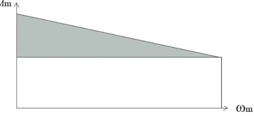
Normally, the motor's performance curve is an horizontal line, that is to say, the output torque does not change along with the speed of the motor. However, for some motors, especially high speed motors, the performance curve is a descending line, which is shown in the Fig. 1.

Fig. 1 Motor's performance curve

If the area of the triangle highlighted in Fig. 1 is small enough, the performance curve is regarded approximately as an horizontal line. The torque given by the motor is always the rated torque. In many cases, this area is quite large due to the great difference of the value of stall torque

𝑀

_𝑀,𝑆 when the motor speed is null and the value of rated torque

𝑀

_𝑀,𝑅 at the rated speed

𝜔

_𝑀,𝑅 .

The output torque decreases when speed increases is due to the fact that at null speed the only energy waste is the intervention of Joule effect, whereas when the speed is different from zero there are also energy wastes due to eddy currents, hysteresis and mechanical losses.

In brushless motors in the out-runner configuration, the radial- relationship between the coils and magnets is reversed; the stator coils form the center (core) of the motor, while the permanent magnets spin within an overhanging rotor which surrounds the

(6)

stator and rotor plates, mounted face to face. Eddy current loss and hysteresis loss exist due to the interaction of electromagnetic fields. Eddy current loss is proportional to the motor angular speed squared, hysteresis loss is proportional to the motor angular speed and windage losses are proportional to the motor angular speed cubic. It's obvious that when the speed is high, these losses cannot be neglected but contribute to the power loss a lot.

If we want to compute the area of the triangle, whic h represents the energy wastes due to eddy current, hysteresis and mechanical losses, mathematical models should be built to evaluate the losses .

A proper motor and a suitable transmission will be chosen to drive a specific periodic load. One of the major problems in the transmission analysis of different motors is the full identification and correct modeling of iron losses, since they affect the performance curve much, especially in high speed mode.

In the conventional approach the limit torque of continuous duty range is constant, which equals to the rated torque

𝑀

_𝑀,𝑅. The new approach takes into account also the iron losses and mechanical losses so as to adjust the limit torque to an accurate and safe one. Correspondingly, the criterion changes. In a specific load and motor case, both the transmission ranges are calculated using Matlab and compared.

(7)

Chapter 1 :Introduction to the conventional

approach

1.1 Scheme of the Drive System

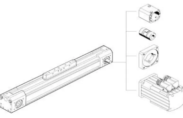
A drive system is a controllable motor with its controller and power driver. In this case, the drive system consists of a PM brushless motor and a linear transmission with a toothed belt, in horizontal position.

Fig. 2 Transmission with toothed belt

The load consists of two components: an implied motion, which is a stroke of the belt and an implied torque.

Fig. 3 shows the scheme of the drive system.

(8)

1.2 Motor Characteristics

Under a specific load, the motor gives a torque with the rotating speed of

𝜔

_𝑚. The moment of inertia of the motor is

𝐽

_𝑀. When the motor works with rated load, the temperature of the motor will increase to a maximum value from the initial temperature when the motor starts. After reaching thermal steady state, the motor can keep functioning well for a quite long time. We call this working range continuous duty working range, with a limit torque

𝑀

_𝑀,𝑆1. When the current in the motor is beyond the rated one, the motor can work for a short time. After a transient time, the motor "burns". If the current is beyond the dynamic limit, the motor "burns" instantaneously. We call this working range dynamic working range, with a limit torque

𝑀

_{𝑀,𝑑𝑦𝑛}. Fig. 4 shows the two ranges:

Fig. 4 Motor working ranges

Below the continuous duty range, the motor works properly for an efficient long time. Between the continuous duty range and dynamic range, the motor can only work for a few hours. This time depends on the sheathing class and the ambient temperature.

𝜔

_{𝑚 𝑡}

0≤𝑡≤𝑇 𝑚𝑎𝑥

(1.1)

then,

𝜔

≤ 𝜔

_{𝑀,𝑚𝑎𝑥}

(1.2)

(10)

1.3.2 Continuous Duty Limits

In continuous duty working range, the limit torque

𝑀

_𝑀,𝑠1 depends on the thermal characteristics of the motor. The motor warms up because of Joule effect (copper losses), hysteresis and parasitic currents (iron losses) and mechanical losses (windage, bearings, etc.).

Although PM brushless motors loose less power than the induction ones, up to 10% of the electrical energy is converted into heat at the rated power of the machine. Heat transfer always occurs when there is a temperature difference in the motor. Due to the power loss, the temperature in the coil is higher than that in the sheathing and air gap or the other parts of the motor. Heat is transferred from the coil windings to the sheathing.

In the coil windings, the main heat transfer means is conduction. There are two mechanisms of heat transfer by conduction: first, heat can be transferred by molecular interaction, in which molecules at a higher energy level (at a higher temperature) release energy for adjacent molecules at a lower energy level via lattice vibration. The second means of conduction is heat transfer between free electrons. This is typical of liquids and pure metals in particular. As the coil windings are made by copper in most cases, and the number of free electrons, which defines the thermal conductivity of solids directly, in copper is relatively great, this heat transfer means exists in the coil windings. Convection and radiation are negligible in this part.

Heat removal is of equal importance as the electromagnetic design of the machine, because the temperature rise of the machine eventually determines the maximum output power with which the machine is allowed to be constantly loaded. From the sheathing to the coolant flow, the main heat transfer means is convection as a matter of fact that forced convection is, inevitably, the most efficient cooling method if we do not take direct water cooling into account. Convection is defined as the heat transfer between a region of higher temperature(here, the sheathing surface) and a region of cooler temperature (here, a coolant of air) that takes place as a consequence of motion of the cooling fluid relative to the solid surface.

The heat generated in the coil windings and the heat removal by the coolant air can be in a dynamic equilibrium. If the loss is too much that beyond the capacity of the

(11)

Fig. 6 Temperature limit of the motor

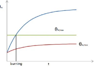
It's possible that the motor is not at thermal steady state, that the internal temperature increases asymptotically to the steady state temperature

_𝑀,𝑆1 is regarded as constant. Fig. 8 shows this limit:

(12)

Fig. 8 𝑀𝑀 ,𝑆1 of the motor

The output torque

𝑀

₀ is less than the limit value

𝑀

_𝑀,𝑆1, that

𝑀

₀

≤ 𝑀

_𝑀,𝑆1

(1.3)

If the mechanical behavior of the motor is periodic with period T and steady state condition is satisfied, a good approximation can be made if the following three conditions are satisfied:

1)

T<<

𝑇

_𝑡ℎ

(1.4)

that the period is far less than thermal transient time

𝑇

_𝑡ℎ: in this condition the motor warming up depends on the average wasted power

𝑊

_𝑤 in the period, and not on the instantaneous power, which varies significantly in the period. In PM brushless motors, thermal transient time

𝑇

_𝑡ℎ lasts for more or less

4𝜏

_𝑡ℎ

,

where

𝜏

_𝑡ℎ is the transient time constant, which usually has the order of one hour. The temperature transient is shown in Fig. 9.

(13)

The load period is always less than one second. So this condition is satisfied. 2) the motor torque is proportional to the current:

𝑀

_𝑀

= 𝐾

_𝑇

𝑖 ;

(1.5)

After testing, which will be explained more clearly later, we find in Fig. 8, that the motor torque is roughly proportional to the current in most of the current range, that is to say, the torque constant

𝐾

_𝑇 can be regarded as constant approximately in our case. This condition is satisfied.

3) the motor wasted power

𝑊

_𝑤 is only due to the Joule effect:

𝑊

_𝑤

= 𝑅𝑖

2

_(1.6)

where

𝐾

_𝑇 is torque constant of the motor,

R

is the resistance at terminals and

i

is the current in the coil.

This is the important assumption of the conventional approach. In fact, the resistance of the coil windings is not constant but increases with temperature. A temperature rise of 50 ℃ above ambient (20℃) increases the resistance by 20% and a temperature rise of 135 ℃ by 53% for copper. If the current of the machine remains unchanged, the resistive losses increase accordingly. Normally, for copper coils, the higher the current flows in it, the higher temperature is in thermal steady state, hence the larger resistance is. Correspondingly, the power loss reaches the maximum when the resistance is the maximum for each single current case. In other words, we can say that if we use maximum resistance to define the limit curve, the safest motor working condition is ensured.

Root mean square motor torque is defined as:

𝑀

_{𝑚,𝑟𝑚𝑠}

=

1

𝑇

𝑀

𝑚2

(𝑡)𝑑𝑡

𝑇

0

(1.7)

Average wasted power is defined as:

𝑊

_𝑤

=

𝐸

𝑤

𝑇

=

1 𝑇

𝑊

𝑤

𝑡 𝑑𝑡 =

1 𝑇

𝑅𝑖

2

𝑡 𝑑𝑡

𝑇 0 𝑇 0

=

𝑅 𝑇 𝑀_𝑚2 (𝑡) 𝐾2

𝑑𝑡

𝑇

=

_𝐾𝑅₂ 1_𝑇

𝑀

𝑚2

(𝑡)𝑑𝑡

𝑇 0

(1.8)

(14)

So,

=

𝑊

_𝑤 𝑅

𝐾_𝑇2

𝑀

𝑚,𝑟𝑚𝑠 2

(1.9)

Nevertheless, with a constant torque

𝑀

₀, averaged wasted power in this condition is

=

(𝑡)

.

Under these three conditions, the motor with mechanical periodic behavior does not burn if

(15)

1.3.3 Dynamic Limit

The converter transistors can suffer a maximum peak current without burning for a small time range. Because of the proportionality between

M

_m and

i

, the torque

𝑀

_{𝑀,𝑑𝑦𝑛} corresponds to this current.

𝑀

=

𝑀

_{𝑚 𝑡}

0≤𝑡≤𝑇

𝑚𝑎𝑥

(1.13)

𝑀

≤ 𝑀

_{𝑀,𝑑𝑦𝑛}

(1.14)

1.3.4 Conclusion of the Constraint Inequalities

The three constraint inequalities are:

𝜔

≤ 𝜔

𝑀

≤ 𝑀

𝑀,𝑠1

𝑀

≤ 𝑀

_{𝑀,𝑑𝑦𝑛}

(16)

1.4 Transmission Characteristics

A linear transmission is implied with the ratio

𝜏

and negligible moment of inertia. We can make a reasonable assumption that the transmission ratio is so small that the motor executes many revolutions to drive the load. In practice, this assumption is always satisfied as the period of the load is longer than the rotating period of the motor. There are direct and inverse power flows. In general, the power flows and their relations with efficiencies are very complex. Since we have neglected the moment of inertia of the transmission, a conclusion can be made that when the load torque has the same rotating direction with the angular speed, the drive system has the direct efficiency. On the contrary, when the load torque has the opposite rotating direction with respect to the angular speed, the drive system has the inverse efficiency. Fig.10 shows the structure of the transmission:

(17)

1.5 Load Specification

Considering the efficiencies of transmission, the torque load is modified.

𝑀

_𝐿∗ is introduced.

𝑀

_𝐿∗

₌

𝑀_𝐿 𝜂_𝑑

𝑖𝑓 𝑀

𝐿

𝑤

𝐿

> 0;

(18)

𝑀

=

1 𝑇

[

𝐽_𝑀𝛼_𝐿 𝑡 𝜏

+ 𝜏𝑀

𝐿 ∗

_(𝑡)]

2 𝑇 0

𝑑𝑡 ≤ 𝑀

_𝑀,𝑆1

(1.21)

𝜔

=

𝜔𝐿,𝑚𝑎𝑥 𝜏

≤ 𝜔

𝑀,𝑚𝑎𝑥

(1.22)

From equations (1.20), (1.21) and (1.22), three intervals of

𝜏

are obtained separately. The reasonable and safe solution of the transmission ratio for the specific load is the intersection of these intervals.

(19)

Chapter 2: Losses in Brushless Motors

Power losses are important because they determine the efficiency and the temperature-rise of the machine. The two most important components of power loss are the Joule loss in the stator conductors and the iron loss, most of which is in the stator laminations. The iron loss is roughly proportional to the square of the product of flux and frequency. Consequently it is relatively more significant at high speed and/or light load, whereas the Joule loss is often predominant at low speed.

In PM machines, Joule loss is called copper loss as well, due to the fact that most Joule loss exists in the copper- made coil windings. The Joule loss consists of two parts: external Joule loss and internal Joule loss. The former is related to the output torque, or more essentially, to the load case. The latter is related to resistant torque given by eddy current, hysteresis and mechanical losses.

Permanent magnet excited machines are undoubtedly energy efficient, while the brushless dc format is emerging as the most significant for many applications. However, the stator iron losses depend on numerous design and fabrication factors, such as the grade of lamination material, the number of poles, operational conditions such as the type of supply converter and the load, heat treatment, burrs, interlaminar insulation etc.

Windage and friction losses are similar to those in induction motors. To the extent that a PM machine may have a slightly larger air gap than a comparable induction motor, the windage loss will be lower. PM machine often does not need a fan, in which case the associated "fan losses" will be avoided.

Similarly to the previous approach, maximum resistance is applied to the equations for the sake of ensuring the safe working condition.

(20)

2.1 External Joule Losses

The main term of Joule losses is external loss, which is related to the output torque

𝑀

_𝑚 of the motor. The current 𝑖 in the coils can be calculated by

𝑖 =

𝑀𝑚

𝐾_𝑇

(2.1)

The external Joule losses can be written as:

𝑃

_𝐽

= 𝑅𝑖

2

= 𝑅

𝑀𝑚

𝐾_𝑇 2

= 𝑅

𝑀𝑚2

𝐾_𝑇2

(2.2)

where

𝑅

is the maximum resistance in the terminals of the coil windings as what is said previously.

(21)

2.2 Hysteresis Loss

Hysteresis loss is a heat loss caused by the magnetic properties of the armature. When an armature core is in a magnetic field, the magnetic particles of the core tend to line up with the magnetic field. When the armature core is rotating, its magnetic field keeps changing direction, with a frequency f. The continuous movement of the magnetic particles, as they try to align themselves with the magnetic field, produces molecular friction. This, in turn, produces heat. This heat is transmitted to the armature windings. The heat causes armature resistances to increase. Steel of the iron core is very good ferromagnetic material. This kind of materials are very sensitive to be magnetized. That means whenever magnetic flux passes through, it will behave like magnet. Ferromagnetic substances have numbers of domains in their structure. Domain are very small region in the material structure, where all the dipoles are paralleled to same direction. In other words, the domains are like small permanent magnet situated randomly in the structure of substance. These domains are arranged inside the material structure in such a random manner, that net resultant magnetic field of the said material is zero. Whenever external magnetic field or MMF is applied to that substance, these randomly directed domains are arranged themselves in parallel to the axis of applied MMF. After removing this external MMF, maximum numbers of domains again come to random positions, but some of them still remain in their changed position. Because of these unchanged domains the substance becomes slightly magnetized permanently. This magnetism is called " Spontaneous Magnetism". To neutralize this magnetism some opposite MMF is required to be applied. The MMF applied in the iron core is alternating. For every cycle, due to this domain reversal there will be extra work done. For this reason, there will be a consumption of electrical energy which is known as hysteresis loss. Physically the hysteresis loss is caused by very localized irreversible changes during the magnetization process, which make it dependent only on the maximum induction. Hysteresis loss results from the "unwillingness" of the steel to change its magnetic state. Through one electrical cycle the magnetic represented by the point (H,B) describes a closed loop in the B/H diagram, Fig. 11.

𝐵

_𝑚 curve derived experimentally from single-sheet 'dc' tests. In most cases,

𝛼

can be from 1.5 to 2. From equation 2.1 we know that hysteresis loss is related to the amplitude of the flux density.

In PM brushless motors, flux density is depended on the material of the permanent magnets. For a certain motor, we can assume that

𝐵

_𝑚 is constant and can be known from the motor user manual. Hysteresis loss is proportional to the frequency

𝑓

,then

(23)

_𝑚

+ 𝑅

𝑀ℎ

2

(24)

2.3 Eddy Current Loss

Eddy currents are electric currents induced within conductors by a changing magnetic field in the conductor. When current is induced in a conductor such as the square piece of metal shown above, the induced current often flows in small circles that are strongest at the surface and penetrate a short distance into the material. These current flow patterns are thought to resemble eddies in a stream, which are the tornado looking swirls of the water that we sometimes see. Because of this presumed resemblance, the electrical currents were named eddy currents. When current flows through the solenoid, the magnetic flux linked to the solenoid increases from zero to finite value. This change in magnetic flux gives rise to induced currents in the disc upon the upper surface of the iron core. When a conductor is kept in a changing magnetic field, current are induced in the body of the conductor. The currents occur in very small loops, and are called eddy currents. The direction of induced current is such as to oppose the very cause producing it, stated in Lenz's Law. These eddy currents cause local temperature increases, known as eddy current loss. The eddy current loss that is induced in the permanent magnets of brushless machines is often neglected. However, this assumption may not always be justified. For example, machine designs are emerging in which the torque is produced by the interaction of a space-harmonic magnetomotive force (MMF) with the permanent magnets and which employ concentrated windings. Although this results in short end-windings, and, hence, a low copper loss, and a high power density, and the coils may be wound only on alternate teeth so as to enhance fault-tolerance, eddy currents will be induced in the magnets by forward and backward rotating MMFs. The situation may be aggravated further by time harmonics in the phase currents. Due to the relatively high electrical conductivity of rare-earth magnets, the resultant eddy-current loss can be significant, and may cause a substantial temperature rise and result in partial irreversible demagnetization of the magnets, especially in machines with a high electric loading, a high rotational speed, or a high pole number. These circulating eddies of current have inductance and thus induce magnetic fields. These fields can cause repulsive, attractive, propulsion, drag and heating effects. The stronger the applied magnetic field, or the greater the electrical conductivity of the conductor, or the faster the field changes, then the greater the currents that are developed and the greater the fields

(25)

_𝑒 decreases by half. Similarly,

𝐵

_𝑝𝑘 is depend on the material of the permanent magnets and independent of the current.

Since

𝑘

_𝑒

and

2.4 Mechanical Losses

Mechanical losses usually consist of windage, friction and bearing losses. The power transmission cannot be achieved without losses or dissipation of heat within the transmission. Among these losses we can distinguish those by friction resulting from contact between teeth in mesh which constitute a major source of dissipation at low rotational speeds . The other important loss is that caused by churning which represents the power lost because of the compress ion of the air-lubricant mixture around teeth roots during meshing. The third power loss is that induced by windage which corresponds to the power lost because of the aerodynamic trail of the teeth in the air- lubricant mixture. It is assumed that the windage loss controls the total efficiency of the system in the case of high operating speeds. So, these power losses must be taken into account in order to choose the optimized transmission and motor. Except in high-speed motors, losses caused by friction and windage are very low in PM brushless motors, typically accounting for less than one or two percents of the total losses.

Friction losses can be divided into dry friction and viscous friction. The form of dry friction is exactly the same as the hysteresis loss and viscous friction is the same as the eddy current loss. So we just consider them contained in the hysteresis loss and eddy current loss to simplify the case. The mechanical losses can be written as:

𝑃

_𝑚

= 𝑤𝜔

_𝑚3

(2.14)

Similarly, the mechanical loss causes Joule effect like hysteresis loss. This part of Joule loss is

𝑃

_𝑚,𝐽

= 𝑅

𝑤𝜔𝑚

2 2

𝐾_𝑇2

(2.15)

(27)

All the losses are calculated separately. They are classified into two categories, internal losses and external losses.

_𝑚.

2.5 Testing

The importance of physical testing is self-evident for all electrical machines. It includes the design and assembly of dynamometers and other test fixtures; the acquisition and sometimes the design of measuring instruments; a knowledge of standards and standard procedures; a high standard of organization and record-keeping; and above all a meticulous attention to detail, both in the operation of the tests and in the observation of process and results. The objectives of testing are to check that the product is fit for delivery to the customer or not and to identify certain parameters which are difficult to measure directly on the machines. For our case, resistance testing, EMF testing and torque testing are necessary.

(28)

2.5.1 Resistance Testing

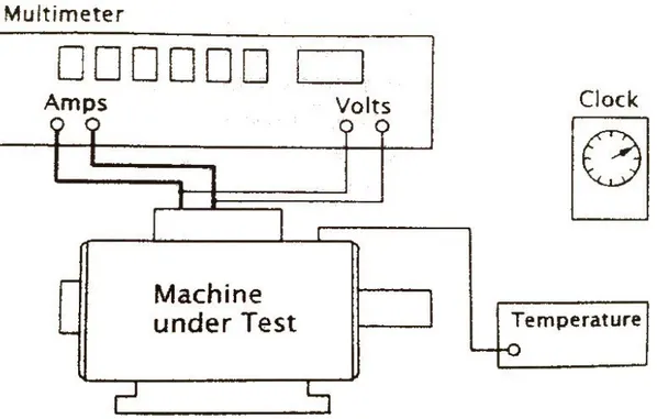
The simplest way to measure winding resistance is to use a multimeter with "4-terminal" resistance measurement, which is altogether the most accurate method. The winding temperature must be measured at the same time as the resistance, because the accuracy of the resistance measurement is only as good as the accuracy of the temperature. See Fig. 12.

Fig. 12 Resistance measurement

In this test, we get the maximum resistance

R

, which ensures the motor does not burn as what is clarified in equation 1.6.

(29)

2.5.2 EMF Testing

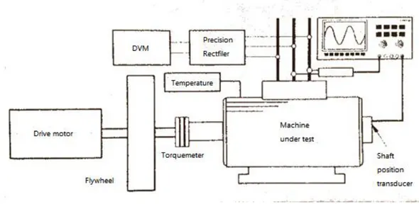
EMF testing is electromagnetic field testing. It is arguably the most important and useful test which can be performed on a brushless PM motor. In many cases, it is the only performance test required on the production line for motor qualification, because the relationship between the EMF and the torque is so predictable. Fig. 13 shows the EMF testing scheme.

Fig. 13 EMF testing

Fig. 13 shows the measurement of the mean rectified EMF using a precision rectifier, as well as the EMF waveform from which the peak line- line EMF is obtained. It thus provides for both the preferred methods of defining and measuring the EMF constant

𝐾

_𝐸

.

(30)

2.5.3 Torque Testing

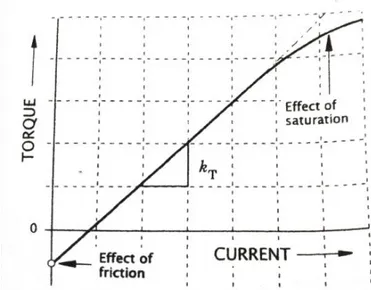
The torque linearity can be tested on a setup such as the one in Fig. 13, preferably with a load machine or brake that can be programmed with torque. A typical result is shown in Fig. 14.

f

Fig. 14 Measurement of torque constant 𝐾_𝑇

Even though non linearity exist in low current and high current condition due to friction and saturation, we can consider

𝐾

_𝑇 is constant for most cases the rated current is in the medium range. This test can be evident to the assumption 2 in chapter 1.3.2, equation 1.5.

Normally,

K

_T is quoted in catalogue data of the motor and slightly deduced from a measured value of

𝐾

_𝐸 due to the non-linearity.

Since we have known the input power of the drive motor and the output torque and power from the sensor of the machine under test, the losses are obtained. In the

(31)

Fig. 15 Hysteresis resistant torque

As this torque is constant, we can regard it as a friction.

Eddy current loss is characterized as a resistant torque, whose value is

𝑟

_𝑒

𝜔

_𝑚, multiplied by the speed of the machine. Fig. 16 shows the resistant torque

𝑟

_𝑒

𝜔

_𝑚

Fig. 16 Eddy current resistant torque

As this torque is proportional to the speed, we can regard it as viscous.

Mechanical losses are characterized as a quadratic resistant torque multiplied by the speed of the machine. Fig. 17 shows the resistant torque.

(32)

Fig. 17 Mechanical resistant torque

As this torque is proportional to the speed squared, we can regard it as an inertia. So the total loss is the sum of the hysteresis, eddy current and mechanical losses. In the Fig., we superimposition of the three parts:

(33)

Chapter 3: New Approach

In the conventional approach, there are three inequalities to be defined as the criterion in choosing the transmission ratio. In the new approach, the speed limit and dynamic limit are the same. The only difference is that the continuous duty limit is changed as iron losses and mechanical losses are taken into account. Now we focus on the continuous duty limit.

3.1 Performance Curve of the Motor

The maximum wasted power during work is no longer constant but increases with the angular speed of the motor. Resulted in this, the performance of the motor is a descending curve. In conventional approach, only the maximum Joule loss is taken into account. Hence the limit torque is constant. By contrast, the new approach takes into account iron losses and mechanical losses at any single angular speed. As a result, the limit curve is no longer constant but a descending curve because the losses increase with the speed. A qualitative curve is shown in Fig. 19:

Fig. 19 Comparison of motor performances in the two approaches

It is reasonable that the total loss has an upper bound, otherwise the motor cannot work regularly. This limit depends on the sheathing class of the motor. The insulation materials can be classified with respect to the heat capability to seven classes: y, a, e, b, f, h, c. Corresponding maximum operating temperatures are 90℃, 105℃, 120℃, 130℃, 155℃, 180℃ and above 180℃. The resistance at the terminals of the coils is the maximum at this operating temperatures. Based on experience, a-class materials can work properly at 105℃ up to 10 years. As the environment temperature and operating temperature are not at the maximum designed temperature, the life of the

(34)

temperature, the sheathing gets aged significantly. Hence operating temperature and the sheathing class are the main parameters to define the maximum wasted power, which is converted into heat. This power limit

𝑖

𝜔

𝑚

≤ 𝑊

𝑙𝑖𝑚

(3.2)

that is:

_𝐾𝑅 𝑇2

𝑀

𝑙𝑖𝑚 2

(3.3)

𝑀_𝑚,𝑒 ≤ 𝑀_𝑙𝑖𝑚2 ₋𝐾𝑇2 𝑅 𝑀ℎ𝜔𝑚 + 𝑟𝑒𝜔𝑚2 + 𝑤𝜔𝑚3 − 𝑀ℎ+ 𝑟𝑒𝜔𝑚 + 𝑤𝜔𝑚 2

(3.4)

(35)

So the equation becomes

𝑀

_𝑚,𝑒

≤ 𝑀

_𝑙𝑖𝑚2

−

𝐾𝑇

2

𝑅

𝑀

ℎ

𝜔

𝑚

+ 𝑟

𝑒

𝜔

𝑚2

+ 𝑤𝜔

𝑚3

𝑀_𝑚,𝑒,0 is known as stall torque 𝑀_𝑠, which means that the angular speed of the motor is null. So

𝑀

_𝑙𝑖𝑚

= 𝑀

_𝑠

(3.8)

This is the first solution of the parameters. Based on this, the other parameters are solved mathematically.

(36)

3.3.2 Solution of

𝑴

_𝒉

, 𝒓

_𝒆

and 𝒘

We rewrite the equation 3.6 as

𝑀

_𝑚,𝑒2

_{≤ 𝑀}

𝑠2

−

𝐾𝑇 2 𝑅

𝑀

ℎ

𝜔

𝑚

+ 𝑟

𝑒

𝜔

𝑚 2

_{+ 𝑤𝜔}

𝑚3

(3.9)

that is

𝐾𝑇2 𝑅

𝑀

ℎ

𝜔

𝑚

+ 𝑟

𝑒

𝜔

𝑚 2

_{+ 𝑤𝜔}

𝑚3

≤ 𝑀

𝑠2

− 𝑀

𝑚,𝑒2

(3.10)

Now 𝐾𝑇 2 𝑅

,

𝑀

𝑠 2

and

𝑀

_𝑚,𝑒2 are known, the parameters

𝑀

_ℎ

, 𝑟

_𝑒 and

𝑤

)

= 𝑀

𝑠2

− 𝑀

𝑚,𝑒32

(3.11)

(37)

3.4 Representation in the Plane

𝝎

_𝒎

− 𝑴

𝜔

𝑚2

+ 𝑤𝜔

𝑚3

𝑑𝑡

𝑇

In the no load condition, we can easily solve this equation. At each angular speed of the motor, we get a point (

𝜔

_𝑚0

, 𝑀

_𝑒) on the Torque-Speed diagram. A qualitative plot is shown in Fig.20:

(38)

3.5 Load Representative Point

With the specific load we have defined previously, the motor does not work in steady state condition. Integrations of the total loss in the period with respect to time are used, with the specific load:

𝑀

_𝑚,𝑒

=

𝐽𝑀 𝜏

𝛼

𝐿

𝑡 + 𝜏𝑀

𝐿 ∗

_(𝑡)

_(3.14)

and

𝜔

_𝑚

=

𝜔𝐿 𝜏

(3.15)

The equation 3.6 becomes

1 𝑇 𝐽𝑀 𝜏 𝛼𝐿 𝑡 + 𝜏𝑀𝐿 ∗_(𝑡) 𝑇 0 2 𝑑𝑡 + 1_𝑇 𝐾𝑇2 𝑅 𝑀ℎ 𝜔𝐿 𝜏 + 𝑟𝑒 𝜔𝐿 𝜏 2 + 𝑤 𝜔𝐿 𝜏 3 𝑑𝑡 𝑇 0 ≤ 𝑀_𝑠2

_(3.16)

1 𝑇

𝐽_𝑀2 𝜏2

𝛼

𝐿2

𝑡 + 𝑀

𝐿∗2

𝑡 𝜏

2

+ 2𝐽

𝑚

𝛼

𝐿

𝑡 𝑀

𝐿∗

𝑡

𝑇 0

𝑑𝑡 +

1 𝑇 𝐾_𝑇2 𝑅

𝑀

ℎ

𝜔_𝐿 𝜏

+ 𝑟

𝑒 𝜔_𝐿 𝜏 2

+ 𝑤

𝜔𝐿 𝜏 3

𝑇 0

𝑑𝑡 ≤ 𝑀

𝑠 2

(3.17)

As is known,

1 𝑇

𝐽_𝑀 𝜏

𝛼

𝐿

𝑡 + 𝜏𝑀

𝐿 ∗

_(𝑡)

𝑇 0 2

𝑑𝑡 = 𝑀

𝑚,𝑟𝑚𝑠2

(3.18)

(39)

characterize the working condition.

Hence both the two variables

𝜔

_𝑚0 and

𝑀

_{𝑚,𝑟𝑚𝑠} are known, we can plot the couple of variables in the Plane

𝜔

_𝑚

− 𝑀

_𝑚

,

as shown in Fig.21:

Fig.21 Equivalent working point with load

3.6 Effect of the Transmission Ratio

After an interval of transmission ratio

𝜏

is given, say [0.0001,10], two corresponding series of

𝑀

and

𝜔

_𝑚0 are obtained by solving equation 3.16 and equation 3.17. Consequently, we get the feasibility curve. A qualitative plot is shown in Fig.22:

(40)

represents the motor losses(the blue one), the solutions of transmission ratio are obtained. In the interval of transmission ratio defined by the feasible arc, the drive system works without burning.

Along with the other inequalities, that

𝑀

_{𝑚 ,𝑚𝑎𝑥}

=

(

𝐽𝑚𝛼𝐿(𝑡) 𝜏

+ 𝜏𝑀

𝐿 ∗

_{(𝑡) )}

0≤𝑡≤𝑇𝑚𝑎𝑥

≤ 𝑀

𝑀,𝑑𝑦𝑛

𝜔

=

𝜔𝐿 ,𝑚𝑎𝑥 𝜏

≤ 𝜔

𝑀,𝑚𝑎𝑥

(3.21)

(41)

Chapter

4:

Choice

of

Motor

and

Transmission

Servomotor AC brushless series 8C are famous and reliable brushless PM motors. We choose N 501055 - 8C4430 as our objective of study. This is the picture of the motor:

Fig.23 Motor N 501055 - 8C4430

4.1 Corresponding Values of the Parameters

On the website, we can find the catalogue s and user manual of this motor. Fig.23shows the performance of the motor. On the plot we can easily check the dynamic limit, which is the green line and the continuous duty limit, which is the red line.

It is obvious the continuous duty limit is a descending line, as analyzed in the new approach.

(42)

Fig.24 Characteristic curve of the motor

The procedure of obtaining this curve is:

1) Set a maximum temperature

𝜃

,

below which the motor does not burn; 2)Set a speed of the motor. Normally, we start from the stall torque, which means the output torque when the motor works at null speed;

3)Drive the motor in the no load EMF test to thermal steady state, i.e. after a thermal transient time the temperature stays constant;

4)Sense and record the output torque;

5)Increase the motor speed and repeat 3) and 4).

Then we get a series of points on the Torque-Speed diagram step by step. By linking the points in a line, we obtain the motor characteristic curve, which is the continuous duty limit curve in the new approach.

(43)

resistance at terminals

𝑅

, torque constant

𝐾

_𝑇, and stall torque

𝑀

_𝑠. They are highlighted in Appendix A and Appendix B.

By now we have all the values of the parameters needed.

4.2 Calculations and Results in Matlab

MATLAB, the language of technical computing, is a programming environment for algorithm development, data analysis, visualization, and numeric computation. The data is processed with MATLAB.

4.2.1 Position, Velocity and Acceleration of the Load

The load acceleration is in the form that constant acceleration with " 1

3

𝑎𝑛𝑑

1 3"

positive acceleration non dimensional time and negative acceleration non dimensional time. T is set to 0.15 second and both the positive acceleration dimensionless time and negative acceleration dimensionless time is 0.3. The stroke of the load

𝑋

_𝐿 is one meter. By integrating the acceleration once and twice with respect to time in the period, we get the velocity and position. Acceleration is

𝛼

_𝐿and velocity is

𝜔

𝑟

_𝑒 = 0.00014914

𝑤

= 2.4404e-007

As

𝑟

_𝑒 and

𝑤

are quite small, they only affect the shape of the characteristic curve of the motor at high speed mode. This is consistent with our previous analysis.

4.2.4 Mathematic Solution of

𝑴

_{𝒎,𝒓𝒎𝒔}

and Transmission Ratio

We set transmission ratio

𝜏

is from 0.01 to 50 with an incremental of 0.01.

𝑀

_{𝑚,𝑟𝑚𝑠} is calculated and plotted with the characteristic curve of the motor. The result is shown in Fig. 28:

(46)

output torque will not exceed dynamic limit.

The maximum load speed is 9.5823 m/s as calculated previously. The maximum rated angular speed of the motor is 3000 rpm, that is 314.1593 rad/s. From the inequality that

𝜔𝐿 ,𝑚𝑎𝑥

𝜏

≤ 𝜔

𝑀,𝑚𝑎𝑥

(4.1)

𝜏

_𝑚𝑖𝑛

=

𝜔𝐿,𝑚𝑎𝑥

𝜔_{𝑀 ,𝑚𝑎𝑥}

= 0.030315

From the Fig. 28 it is easy to find the corresponding transmission ratio interval whose lower and upper bounds are the intersections of the two curves.

𝜏

=

0.02,0.97

The final result of transmission ratio

τ

is obtained considering both the two criterions is 0.03 to 0.97 .

In conventional approach,

𝑀

_{𝑚,𝑟𝑚𝑠} is calculated without any iron losses and the continuous duty limit is the rated torque. We call it

𝑀

_{𝑚,𝑟𝑚𝑠0} in order to distinguish. The two plots are shown in the same Fig. 29:

(47)

Fig. 30 Zoom of acceptable transmission ratio zone

we can find that the two transmission ratio intervals are quite different. The interval due to continuous duty limit using the conventional approach is

𝜏

=

0.04,0.63

Considering

𝜏

_𝑚𝑖𝑛

= 0.030315, t

he final result of the conventional

approach

is

𝜏

=

0.04,0.63

.

If we decrease the period and keep other load specifications unchanged, it is obvious that the whole level of root mean square torque is improved. As a result, we can propose that the conventional approach will give no solution while the new approach will give an efficient solution.

Now we decrease the period from 0.15 second to 0.05 second, new results are shown in Fig.31:

(48)

If we zoom it to recognize the available interval, as shown in Fig.32:

Fig. 32 Zoom of comparison of the two approaches

We can see that the results are consistent with our assumption well.

(49)

Chapter 5: Conclusions and Discussions

After series of research and tests based on the assigned motor and transmission, three conclusions can be made:

1) iron losses and mechanical losses can be significant when the motor angular speed is high;

2) the new approach gives a more accurate, practicable and beneficial solution than the conventional approach does when both the approaches are valid;

3) the new approach can even give a solution when the load is so critical that using the conventional approach no solution is obtained.

In order to back these conclusions up, the whole design and test procedure is divided into four parts and explained as follows:

The first part of the study is to analysis the known method. The basic concept is that the wasted energy during the motor works should be less than a limit value. The wasted power is due to Joule loss due to the conventional approach. By calculation, we know that the power loss is equal to the root mean square torque of the motor in a period at steady state. The limit torque is defined as the rated torque of the motor, which is constant. After specifying the periodic load and introducing the relationship between load, transmission ratio and the output torque of the motor, we can find the efficient transmission ratio by finding the intersections of the equivalent power loss curve and the limit curve.

The second part is to identify the hysteresis loss, eddy current loss and mechanical losses. According to the electromagnetic properties of the permanent magnets, hysteresis loss and eddy current loss are identified. Hysteresis loss is related to the amplitude of the flux density and the frequency at which the flux density changes. For the chosen specific motor, the amplitude of the flux density is only depend on the material of the permanent magnets. So it's a constant. The frequency is equal to the angular speed of motor divided by

2𝜋

multiplied by the number of poles of the motor. Hence hysteresis loss is proportional to the speed of the motor. Eddy current loss is a little more complicated. It's related to the peak value of the flux density the frequency powered by Steinmetz constant

𝛼,

which is determined by the material of the permanent magnets. As a convention, we set

𝛼

to 2. That is to say, eddy current loss is proportional to the speed squared. The mechanical losses is proportional to the speed cubic. With these theories, we define the losses in the motor along with the Joule loss.

The third part of the study is to build the mathematic models of the new approach for evaluating the transmission ranges. The basic concept of the new approach is the same with the conventional one. But we consider the maximum losses is determined not only by the Joule loss but also the iron losses and mechanical losses. The limit

(50)

obtained by the catalogue in the user manual. This is the main difference between the two approaches. After introducing internal losses and external losses, we can define a couple of variables

(𝜔

_𝑚0,

𝑀

_{𝑚,𝑟𝑚𝑠}), which is equivalent to root mean square torque representing the losses at the equivalent angular speed

𝜔

_𝑚0

.

By dividing the transmission ratio into a discrete series, a series of points representing the power loss is obtained and the curve can be plotted by linking these points. The transmission ratio interval is got by finding the intersections of these two curves.

The fourth part of this study is to assign the motor and transmission to compare these two approaches and test the theories. After solving the parameters in the new approach and plotting the four curves explained previously, we can easily see the difference of the results of the two approaches. As expected, the new approach gives an enlarged transmission ratio ranges. Sometimes it can give a solution while the conventional approach can't. We can say that a more safe and accurate interval of transmission ratio is obtained compared to the conventional approach. Therefore, the improved approach is very helpful for choosing transmission ratio for PM brushless machine, particularly for high-speed motors. For low-speed motors, the conventional approach gives a good approximation, thus the two approaches consist on the whole. In the future works, to validate the proposed model, laboratory testing on different motor speeds and different motors should be carried out. On the other hand, since the equivalent speed is directly calculated with the parameters of iron losses and mechanical losses, the result of the new approach is highly related to the accuracy of the evaluation of hysteresis, eddy current and mechanical losses. If a more accurate mathematic model of the evaluation of these losses is built, a more accurate result will be obtained.

(51)

Acronyms

PM: permanent magnet

EMI: electromagnetic interference DC: direct current

MMF: magnetomotive force EMF: electromagnetic fields

Internet resources

Wikipedia

http://www.wikipedia.org/

ABB Group

(52)

Literature reference

[1] G.R. SLEMON AND X. LIU, "Core losses in permanent magnet motors", IEEE Transaction on Magnetics, V.26, 1653-1655, 1990

[2] G.R. SLEMON AND R. BONERT C. MI, "Modeling of iron losses of

surface-mounted permanent magnet synchronous motors", Proc. of IEEE IAS

36th Annual Meeting, V.4, 2585-2591, 2001

[3] F. DENG, "An improved iron loss estimation for permanent magnet brushless

machines", IEEE Transactions on Energy Conve rsion, V.14, 1391-1395, 1999

[4] Z. ZHU K. ATALLAH, D. HOWE, "An improved method for predicting iron

losses in brushess permanent magnet DC drives", IEEE Transaction on Magnetics,

V.28, 2997-2999, 1992

[5] T. J. E. MILLER R.RABINOVICI, "Eddy-current losses of surface-mounted

permanent magnet motors", IEE Proc.-Electr. Powe r Appl., V.144, 61-64, January,

1997

[6] G. W. CARTER, "The Electromagnetic Field in its Engineering Aspects, 2nd

edition, Longman", 1967

[7] M. MCGILP D. M. IONEL, T.J. E. MILLER, S.J. DELLINGER AND R.J. HEIDEMANN, "Computation of core losses in electrical machines using improved

model for laminated steel", IEEE Transaction on Industry Applications, V.43,

1554-1564, November/December 2007

[8] P. H. DAWSON, "High-speed gear windage", GEC Review, V.4, 164-167, 1988

[9] G. KANTCHEV F. CHAARI , M. HADDAR, "Numerical computation of

the mechanical efficiency of a spur gear system", Eng. Comp. Mech., V.163, 83-90,

2010

[10] K. SIMMONS K. AL-SHIBL , C. N EASTWICK " Modeling Gear

Windage Power Loss From an Enclosed Spur Gears", Proc. Inst. Mech. Eng., Part

(53)

Acknowledgements

Firstly and fore mostly, I am grateful to my supervisor, Professor Giancarlo Cusimano, whose useful suggestions, incisive comments and constructive criticism have contributed greatly to the completion of this thesis. He de voted a considerable portion of time to reading my manuscripts and making suggestions for further revisions. His tremendous assistance in developing the framework for analysis and in checking the draft versions of this thesis several times as well as his great care in this work deserve more thanks than I can find words to express.

I am also greatly indebted to all the teachers or staffs who have helped me directly and indirectly in this work. Any progress that I have made is the result of their profound concern and selfless devotion.

At last, I must thank my girlfriend Li Sicong and my family. They have given me so much support and courage when I had problems and felt depressed.

(54)

Appendix A

The main electromechanical parameters and data of servomotors 8C under rated voltage of 230V.

(55)

Appendix B

The characteristics of servomotors 8C.