The usual robust control framework in discrete time: some interesting results

QUADERNI DEL DIPARTIMENTO DI ECONOMIA POLITICA E STATISTICA

Marco P. Tucci

The usual robust control framework in discrete time: Some interesting results

Marco P. Tucci*

Abstract: By applying robust control the decision maker wants to make good decisions when his model is only a good approximation of the true one. Such decisions are said to be robust to model misspecification. In this paper it is shown that the application of the usual robust control framework in discrete time problems is associated with some interesting, if not unexpected, results. Results that have far reaching consequences when robust control is applied sequentially, say every year in fiscal policy or every quarter (month) in monetary policy. This is true when unstructured uncertainty à la Hansen and Sargent is used, both in the case of a “probabilistically sophisticated” and a non-“probabilistically sophisticated” decision maker, or when uncertainty is related to unknown structural parameters of the model.

JEL classification: C61, C63, D81, D91, E52, E61

Keywords: Linear quadratic tracking problem, optimal control, robust control, time-varying

parameters.

1. Introduction

Robust control has been a very popular area of research in the last three decades and shows no sign of fatigue.1 _{In recent years a growing attention has been devoted to its continuous}

time version (see, e.g., Hansen and Sargent, 2011, 2016). A characteristic “feature of most robust control theory”, observes Bernhard (2002, p. 19), “is that the a priori information on

*

Dipt. Economia Politica e Statistica, Università di Siena, 53100 Siena, Italy. Tel.: 0577-232620; fax +39-0577-232661. E-mail address: tucci@unisi.it (M.P. Tucci).

1 _{See, e.g., Giannoni (2002, 2007), Hansen and Sargent (2001, 2003, 2007a, 2007b, 2010, 2016), Hansen et al.}

(1999, 2002), Onatski and Stock (2002), Rustem (1992, 1994, 1998), Rustem and Howe (2002) and Tetlow and von zur Muehlen (2001a,b). However the use of the minimax approach in control theory goes back to the 60’s as pointed out in Basar and Bernhard (1991, pp. 1-4).

the unknown model errors (or signals) is nonprobabilistic in nature, but rather is in terms of

sets of possible realizations. Typically, though not always, the errors are bounded in some

way. ... As a consequence, robust control aims at synthesizing control mechanisms that control in a satisfactory fashion (e.g., stabilize, or bound, an output) a family of models.” Then “standard control theory tells a decision maker how to make optimal decisions when his model is correct (whereas) robust control theory tells him how to make good decisions when his model approximates a correct one” (Hansen and Sargent, 2007a, p. 25). In other words, by applying robust control the decision maker makes good decisions when it is statistically difficult to distinguish between his approximating model and the correct one using a time series of moderate size. “Such decisions are said to be robust to misspecification of the approximating model” (Hansen and Sargent, 2007a, p. 27).

Concerns about the “robustness” of the standard formulation of robust control have been floating around for some time. Sims (2001, p. 52) observes that “once one understands the appropriate role for this tool (i.e. robust control or maxmin expected utility), it should be apparent that, whenever possible, its results should be compared to more direct approaches to assessing prior beliefs.” Then he continues, “the results may imply prior beliefs that obviously make no sense … (or) they may … focus the minimaxing on a narrow, convenient, uncontroversial range of deviations from a central model.” In the latter case “the danger is that one will be misled by the rhetoric of robustness to devoting less attention than one should to technically inconvenient, controversial deviations from the central model.”2

Tucci (2006, p. 538) argues, “the true model in Hansen and Sargent (2007a) … is observationally equivalent to a model with a time-varying intercept.” Then he goes on showing that, when the same “malevolent” shock is used in both procedures, the robust control for a linear system with an objective functional having desired paths for the states and controls set to zero applied by a “probabilistically sophisticated” decision maker is identical to the optimal control for a linear system with an intercept following a “Return to Normality” model and the same objective functional only when the transition matrix in the law of motion of the parameters is zero.3 _{He concludes that this robust control is valid only when “today’s}

malevolent shock is linearly uncorrelated with tomorrow’s malevolent” shock” (p. 553). These results are shown to be valid, in a more general setting with arbitrary desired paths,

2 _{See also Hansen and Sargent (2007a, pp. 14−17).}

3 _{By probabilistic sophistication is meant that “in comparing utility processes, all that matters are the induced}

both for a “probabilistically sophisticated” and a non-“probabilistically sophisticated” decision maker and in the presence of a structural model with uncertain parameters in Tucci (2009).

Indeed, it may be pointed out that “the fact that the transition matrix does not appear

in the relevant expression in Tucci (2006, 2009) does not mean that the decision maker does not contemplate very persistent model misspecification shocks.” For instance, the robust

control in the worst case may not depend upon on transition matrix simply because the persistence of the misspecification shock does not affect the worst case! Again the robust decision maker accounts for the possible persistence of the misspecification shocks, and that persistence may affect the evolution of the control variables in other equilibria, but it happens that transition matrix does not play a role in the worst case equilibrium. Moreover, as commonly understood, “the robust control choice accounts for all possible kinds of

persistence of malevolent shocks, which again may take a much more general form than the VAR(1) assumed in Tucci (2006, 2009). It just happens that in the worst-case misspecification shocks are not persistent. While for many possible ‘models’, these misspecification shocks may be very persistent, such models happen to result in lower welfare losses than the worst-case model.” To shed some light on these issues, this paper will further

investigate the characteristics of the most common specification of robust control in discrete time in Economics by explicitly considering the welfare loss associated with the various controls.

The remainder of the paper is organized as follows. Section 2 reviews the standard robust control problem with unstructured uncertainty à la Hansen and Sargent, i.e. a nonparametric set of additive mean-distorting model perturbations. In Section 3 the linear quadratic tracking control problem where the system equations have a time-varying intercept following a ‘Return to Normality’ model is introduced and the solution compared with that in Section 2. Section 4 reports some numerical results obtained using a ‘robustized’ version of MacRae (1972) problem. Then the permanent income model, a popular model in the robust control literature (see, e.g., Hansen and Sargent 2001, 2003, 2007a; Hansen et al. 1999, 2002) is considered (Section 5). The main conclusions are summarized in Section 5.

Hansen and Sargent (2007a, p. 140) consider a decision maker “who has a unique explicitly specified approximating model but concedes that the data might actually be generated by an unknown member of a set of models that surround the approximating model.”4 _{Then the}

linear system

yt+1= Ayt+ But+ Cεt+1 for t = 0,..., ∞, (2.1)

with _yt the n×1 vector of state variables at time t, _ut the m×1 vector of control variables and εt+1 an l×1 identically and independently distributed (iid) Gaussian vector process with mean

zero and an identity contemporaneous covariance matrix, is viewed as an approximation to the true unknown model

yt+1= Ayt+ But+ C(εt+1+ ωt+1) for t = 0,..., ∞. (2.2)

The matrices of coefficients A, B and C are assumed known and _y0 given. 5

In Equation (2.2) the vector _ωt+1 denotes an “unknown” l×1 “process that can feed back in a possibly nonlinear way on the history of y, (i.e.) _ωt+1= g_t(y_t,y_t−1, ...) where _{gt}

is a sequence of measurable functions” (Hansen and Sargent, 2007a, pp. 26-27). It is introduced because the “iid random process ... _(εt+1) can represent only a very limited class of approximation errors and in particular cannot depict such examples of misspecified dynamics as are represented in models with nonlinear and time-dependent feedback of _yt+1 on past states” (p. 26).6 To express the idea that (2.1) is a good approximation of (2.2) the ω’s

are restrained by

4 _{See Hansen and Sargent (2007a, Ch. 2 and 7) for the complete discussion of robust control in the time}

domain.

5 _{Matrix C is sometimes called the “volatility matrix” because, given the assumptions on the ε’s, it “determines}

the covariance matrix C′C of random shocks impinging on the system” (Hansen and Sargent, 2007a, p. 29). It is furthermore assumed, see e.g. page 140 in the same reference, that the pair ( β1/ 2_{A,B ) is stabilizable.}

6 _{When Equation (2.2) “generates the data it is as though the errors in ... (2.1) were conditionally distributed as}

N (ωt+1,Il) rather than as N (0,Il) ... (so) we capture the idea that the approximating model is misspecified

by allowing the conditional mean of the shock vector in the model that actually generates the data to feedback arbitrarily on the history of the state” (Hansen and Sargent, 2007a, pp. 27).

E₀ βt+1_ω′ t+1ωt+1 t=0 ∞

∑

⎡ ⎣ ⎢ ⎤ ⎦ ⎥ ≤ η0 with 0 < β < 1 (2.3)

where _E0 denotes mathematical expectation evaluated with respect to model (2.2) and

conditioned on _y0 and η₀ measures the set of models surrounding the approximating model.7

“The decision maker’s distrust of his model ... (2.1) makes him want good decisions over a set of models ... (2.2) satisfying ... (2.3)” write Hansen and Sargent (2007a, p. 27). The solution can be found solving the multiplier robust control problem formalized as8

max u minω − E0 β t t=0 ∞

∑

_⎡⎣r(y_t,u_t)− θβ ′ω_t+1ω_t+1⎤⎦ ⎧ ⎨ ⎩ ⎫ ⎬ ⎭,

(2.4)

where _r(yt,u_t) is the one-period loss functional, subject to (2.2) with θ, _{0 <}θ* _{<θ ≤∞, a}

penalty parameter restraining the minimizing choice of the _{ωt+1} sequence and θ* _{“a lower}

bound on θ that is required to keep the objective ... (2.4) convex in ... ( _ωt+1) and concave in

ut” (p. 161).9 This problem can be reinterpreted as a two-player zero-sum game where one

player is the decision maker maximizing the objective functional by choosing the sequence for u and the other player is a malevolent nature choosing a feedback rule for a model-misspecification process ω to minimize the same criterion functional.10 _{For this reason, the} multiplier robust control problem is also referred to as the multiplier game.11

The Riccati equation for problem (2.4) “is the Riccati equation associated with an ordinary optimal linear regulator problem (also known as the linear quadratic control problem) with controls _{( ′}u_t ω′_t+1 ′) and penalty matrix on those controls appearing in the

7 _{See Hansen and Sargent (2007a, p. 11).}

8 _{Alternatively the constraint robust control problem, defined as extremize}

−E0[Σt=0 ∞ _βt

r(y_t, u_t)] subject to (2.2)-(2.3), can be solved. When η₀ and θare appropriately related the two “games have equivalent outcomes.”

See p. 32 and Chapters 6−8 in Hansen and Sargent (2007a) for details.

9 _{As noted in Hansen and Sargent (2007a, p. 40) “this lower bound is associated with the largest set of}

alternative models, as measured by entropy, against which it is feasible to seek a robust rule ... This cutoff value of θ... is affiliated with a rule that is robust to the biggest allowable set of misspecifications.” See also Ch. 7 in the same reference and Hansen and Sargent (2001).

10 _{See Hansen and Sargent (2007a, p. 35).}

criterion functional of diag( _{R, −}βθI_l)” (Hansen and Sargent, 2007a, p. 170).12 _{Then, when}

the one-period loss functional is13

r(y_t,u_t)= y_t− y_td t

(

)

′ Q y

(

_t− y_td

)

_{+ 2 y} t− yt d

(

)

′ W u

(

_t− u_td

)

_{+ u} t − ut d

(

)

′ R u

(

_t − u_td

)

(2.5)

with Q a positive semi-definite matrix, R a positive definite matrix, W an n×m array, _ytd _and

ut

d _{the desired state and control vectors, respectively, the robust control rule is derived by}

extremizing, i.e. maximizing with respect to _ut and minimizing with respect to ω_t+1 , the objective functional −E₀ βt_r(y t,ut) t=0 ∞

∑

⎡ ⎣ ⎢ ⎤ ⎦ ⎥

(2.6) with r(y_t,u_t)= y_t− y_td

(

)

′_{Q y} t − yt d

(

)

+ 2 y

(

_t− y_td

)

′ W u t − ut d

(

)

+ u

(

_t− u_td

)

′ R u t− ut d

(

)

(2.7) subject to yt+1= Ayt+ But + Cεt+1 for t = 0,..., ∞ (2.8) where R = R O O −βθI_l ⎡ ⎣ ⎢ ⎤ ⎦ ⎥ , !u_t = ut ω_t+1 ⎡ ⎣ ⎢ ⎢ ⎤ ⎦ ⎥ ⎥ , !B= B C⎡⎣ ⎤⎦, !u d t = u_td 0 ⎡ ⎣ ⎢ ⎢ ⎤ ⎦ ⎥ ⎥ (2.9)

and W = [W O]with O and 0 null arrays of appropriate dimension.

12 _{This is due to the fact that the “Riccati equation for the optimal linear regulator emerges from first-order}

conditions alone, and that the first order conditions for (the max-min problem (2.4) subject to (2.2)) match those for an ordinary, i.e. non-robust, optimal linear regulator problem with joint control process {u_t , ω_t+1 }” (Hansen and Sargent, 2007a, p. 43).

Setting εt+1 = 0 and writing the optimal value of (2.6) as _{− ′}ytPtyt − 2 ′ytpt,14 the

Bellman equation looks like15

− ′y_tP_ty_t− 2 ′y_tp_t = ext u − ′⎡⎣ytQtyt + ′utRtut −βθ ′ωt+1ωt+1+ 2 ′ytWtut + 2 ′ytqt + 2 ′u_tr_t + ′y_t+1P_t+1y_t+1+ 2 ′y_t+1p_t+1⎤⎦ (2.10) with _Pt+1 =βP_t, _Qt =βt_Q, Wt =β t_W, Rt =β t_R, qt =−( Qtyt d _{+ W} tut d_{) and} rt = −(Rtut d +Wt′yt

d_{).16 Then expressing the right-hand side of (2.10) only in terms of y}

t and _ut and

extremizing it yields the optimal control for the decision maker

ut = − R

(

t+ B′Pt+1B

)

−1 B′P_t+1A+ W_t′

(

)

y_t + B′P_t+1Cω_t+1+ B′p_t+1+ r_t ⎡ ⎣⎢ ⎤⎦⎥ (2.11)

and the optimal control for the malevolent nature

ωt+1 = (βθIl − C′Pt+1C) −1_(C′P

t+1Ayt + C′Pt+1But + C′pt+1). (2.12)

It follows that the θ-constrained worst-case controls are17

ut = − Rt+ B′Pt+1 * _B

(

)

−1 B′P_t*_{+1A+ ′W} t

(

)

y_t + B′p_t*_{+1+ r} t ⎡ ⎣ ⎤⎦ (2.13) and18 ω_t+1 =

(

βθI_l − C′P_t+1C

)

−1C′P_t+1 A− B R

(

_t + B′P_t*_+1B

)

−1 _B′P t+1 * _{A+ ′W} t

(

)

⎡ ⎣⎢ ⎤⎦⎥yt

{

−B R

(

_t+ B′P_t*_+1B

)

−1 _B′p t+1 * _{+ r} t

(

)

+ P_t−1_+1p t+1

}

(2.14)

13 _{In Hansen and Sargent (2007a, Ch. 2 and 7) the desired state and control vectors and W are null arrays.}

14 _{Using the deterministic counterpart to (2.6) and (2.8) allows to simplify some formulas by dropping constants}

from the value function without affecting the formulas for the decision rules (Hansen and Sargent, 2007a, p. 33).

15 _{The constant term appearing on the right-hand side and on the left-hand side of the equation have been dropped}

because they do not affect the solution of the optimization problem. See, e.g., Eqt. (2.5.3) in Hansen and Sargent (2007a, Ch. 2).

16 _{When the desired paths for the states and controls are set to 0,}

pt = qt = rt = 0 .

with19 Pt+1 * _{= I} n+ Pt+1C(βθIl− C′Pt+1C)−1C′ ⎡⎣ ⎤⎦Pt+1 (2.15a) pt+1 * _{= I} n+ Pt+1C(βθIl − C′Pt+1C)−1C′ ⎡⎣ ⎤⎦pt+1. (2.15b)

The “robust” Riccati arrays _Pt*_{+1 and} pt+1

* _{are always greater than, or equal to, P}

t+1 and pt+1,

respectively, because it is assumed that, in the “admissible” region, the parameter θ is large enough to make ₍βθI_l − C′P_t+1C) positive definite.20 _{They are equal when} θ = _∞.21

3. Optimal control of a linear system with time-varying parameters

Tucci (2006, pp. 538-539) argues that the model used by a “probabilistically sophisticated’ decision maker to represent dynamic misspecification, i.e. Eqt. (2.2), is observationally equivalent to a model with a time-varying intercept. When this intercept is restricted to follow a ‘Return to Normality’ or ‘mean reverting’ model,22 _{and the symbols are as in Section 2, the}

latter takes the form yt+1= A1yt + But + Cαt+1 for t = 0,..., ∞, (3.1) with αt+1= a + νt+1 for t = 0,..., ∞, (3.2a) νt+1 = Φνt+ εt+1 for t = 0,..., ∞, (3.2b)

18 _{See, e.g., Eqt. (7.C.9) in Hansen and Sargent (2007a, p. 168).}

19 _{See, e.g., Eqs. (2.5.6) on p. 35 and (7.C.10) on p. 168 in Hansen and Sargent (2007a) where the quantity}

β−1Pt+1 *

is denoted by D(P).

20 _{See, e.g., Theorem 7.6.1 (assumption v) in Hansen and Sargent (2007a, p. 150). The parameter θ is closely}

related to the risk-sensitivity parameter, say σ , appearing in intertemporal preferences obtained recursively. Namely, it can be interpreted as minus the inverse of σ . See, e.g., Hansen and Sargent (2007a, pp. 40−41, 45 and 225), Hansen et al. (1999) and the references therein cited.

21 _{The first order conditions for problem (2.10) subject to (2.8) imply the Riccati equations}

Pt = Qt+ ′A Pt+1 * _{A− A P′} t+1 * _{B+ W} t

(

)

(

R_t+ B′P_t*_+1B

)

−1 _{A P′} t+1 * _{B+ W} t

(

)

′ pt = qt+ ′A pt+1 * _{− ′} A P_t*₊₁B+ W_t

(

)

(

B P′ _t*₊₁B+ R_t

)

−1

(

B p′ *_t+1+ r_t

)

(Hansen and Sargent, 2007a, p. 11).

where a is the unconditional mean of _αt+1, Φ the l×l stationary transition matrix and _εt+1 a Gaussian iid vector process with mean zero and an identity covariance matrix. Matrix _A1 is such that _A1y_t + Ca in (3.1) is equal to Ay_t in (2.2).23 _{In this case, a decision maker}

insensitive to robustness but wanting to control a system with a time-varying intercept can find the set of controls u_t which maximizes24

J = E₀ − L_t

(

y_t, u_t

)

t=0 ∞

∑

⎡ ⎣ ⎢ ⎤ ⎦ ⎥ (3.3)

subject to (3.1)-(3.2) using the approach discussed in Kendrick (1981) and Tucci (2004). When the same objective functional used by the robust regulator is optimized, _Lt is simply the one-period loss functional in (2.5) times βt_.

This control problem can be solved treating the stochastic parameters as additional state variables. When the hyper-structural parameters a and Φ are known, the original problem is restated in terms of an augmented state vector z_t as: find the controls u_t

maximizing25 J = E₀ − L_t

(

z_t, u_t

)

t=0 ∞

∑

⎡ ⎣ ⎢ ⎤ ⎦ ⎥ (3.4) subject to26 zt+1= f(zt,ut)+ εt+1 * _{for t = 0,..., ∞, (3.5)}

22 _{See, e.g., Harvey (1981).} 23 _{When a is a null vector,}

A1≡ A. If a is not zero, A1 is identical to A except for a column of 0’s associated with

the intercept and Ca is identical to the column of A associated with the intercept. It is apparent that, when

ωt+1 ≡ Φνt, the robust control formulation and model (3.1)-(3.2) coincide.

24 _{Kendrick (1981, Ch. 10) analyzes the case where a = 0 and the hyperstructural parameter Φ is known. Tucci}

(2004) deals with the case where a and Φ are estimated.

25 _{See Kendrick (1981, Ch. 10) or Tucci (2004, Ch. 2).}

26 _{When the error term is assumed iid it is equivalent to write the system equations as in (3.5) or as in Tucci}

with27 z_t = yt α_t+1 ⎡ ⎣ ⎢ ⎢ ⎤ ⎦ ⎥ ⎥, f z

(

t, ut

)

= A₁y_t+ Bu_t + Cα_t+1 Φα_t+1+ I

(

_l − Φ

)

a ⎡ ⎣ ⎢ ⎢ ⎤ ⎦ ⎥ ⎥ and εt * ₌ 0 ε_t ⎡ ⎣ ⎢ ⎤ ⎦ ⎥. (3.6)

and the arrays z_t and f(z_t, u_t) having dimension n+l, i.e. the number of original states plus the number of stochastic parameters. For this ‘augmented’ control problem the L’s in Eqt. (3.4) are defined as L_t

( )

z_t,u_t = z_t − z_td

(

)

′_Q t * _z t− zt d

(

)

+ 2 z

(

_t − z_td

)

′_W t * _u t− ut d

(

)

+ u

(

_t − u_td

)

′_R t ut− ut d

(

)

(3.7) with _Qt*_=βt_Q*_, Q*= diag( Q, −βθIl), Wt * _=βt_{[W′ O′ ′] and} Rt =β t_R.

By replacing A₁y_t + Cα_t+1 with Ay_t + Cν_t+1 in (3.6), defining _νt+1 = ω_tc_{+1+ ε}

t+1 with

ωt+1

c _{≡ Φν}

t and using the deterministic counterpart to (3.4)-(3.7),28 namely

zt+1= A * z_t + B* u_t for t = 0,..., ∞, (3.8) with z_t = yt ω_tc₊₁ ⎡ ⎣ ⎢ ⎢ ⎤ ⎦ ⎥ ⎥, A * ₌ A C O Φ ⎡ ⎣ ⎢ ⎤ ⎦ ⎥ and B* =⎡_OB ⎣ ⎢ ⎤ ⎦ ⎥ , (3.9)

the optimal value of (3.4) can be written as _{− ′}z_tK_tz_t− 2 ′z_tk_t and it satisfies the Bellman equation29

27 _{Equations (3.2) are rewritten as α}

t – a = Φ(αt-1 –a) + εt in (3.6). In Tucci (2006, p. 540), the symbol α_t should

be replaced by

αt+1and ωt by ωt+1.

28 _{These preparatory steps are needed to keep the following discussion as close as possible to that carried out in}

section 2 and 3.

29 _{As in the previous sections, the constant term appearing on the right-hand side and on the left-hand side of the}

− ′z_tK_tz_t − 2 ′z_tk_t = max u_t − zt − zt *

(

)

′_Q t * _z t − zt *

(

)

⎡ ⎣ ⎢ + ut − ut *

(

)

′_R t ut− ut *

(

)

+2 z

(

_t − z*_t

)

′_W t * _u t− ut *

(

)

+ ′z_t+1K_t+1z_t+1+ 2 ′z_t+1k_t+1⎤ ⎦ ⎥ (3.10)

with _Kt+1=βK_t. Expressing the right-hand side of (3.10) only in terms of _zt and _ut and maximizing it yields the optimal control in the presence of time-varying intercept (or tvp-control) , i.e.30 u_t = − R

(

_t + ′B K_11,t+1B

)

−1 ×⎡_⎣

(

B K′ _11,t+1A+ ′W_t

)

y_t + ′B K

(

_11,t+1C+ K_12,t+1Φ

)

ω_tc_{+1+ ′B k} 1,t+1+ rt

(

)

⎤_⎦ (3.11)

with K₁₁ and K₁₂ denoting the n×n North-West block and the n×l North-East block, respectively, of the Riccati matrix31

K_t = Q_t*_{+ A}*_′K t+1A * − B*_′K t+1A *_{+ W} t *

(

)

′ _R t + B *_′K t+1B *

(

)

−1 B*_′K t+1A *_{+ W} t *

(

)

(3.12) and

k1,t, containing the first n elements of kt, defined as

k1,t = qt + A′k1,t+1− (B′K11,t+1A+ ′Wt)′(Rt + B′K11,t+1B)−1(B′k1,t+1+ rt) . (3.13)

Then the optimal control (3.11) is independent of the parameter θ which enters only the l×l South-East block of K, namely

K22,t.

When _ωtc_{+1≡ ω}

t+1, i.e. the same shock is used to determine both robust control and

tvp-control, the latter is

30 _{See also, e.g., Kendrick (1981, Ch. 2 and 10) and Tucci (2004, Ch. 2).} 31 _{See Tucci (2004, pp. 26−27). It should be stressed that}

K12,t = (A′K11,t+1C+ A′K12,t+1Φ) − (B′K11,t+1A

+ ′Wt)′(Rt + B′K11,t+1B)−1B′(K11,t+1C+ K12,t+1Φ), then even when the terminal condition for K12 is a null

u_t = −(R_t+ B′K_11,t+1+ _B)−1_[(B′K 11,t+ +1A+ Wt′)yt + B′K11,t+1+ K11,t+1 −1 _k 1,t+1+ rt] (3.14) with K11,t+1 + _{= [I} n+ (K11,t+1C+ K12,t+1Φ)(βθIl − C′Pt+1C) −1_C′]K 11,t+1. (3.15) The quantity

K11,t+1+ collapses to the ‘robust’ Riccati matrix _Pt+1

* _when

Pt+1= K11,t+1 and Φ is

a null matrix because the array

K12,t+1 is generally different from zero. This means that the

control applied by the decision maker who wants to be “robust to misspecifications of the approximating model” implicitly assumes that the ω’s in (2.2) are serially uncorrelated. Alternatively put, given arbitrary desired paths for the states and controls, robust control is “robust” only when today’s malevolent shock is linearly uncorrelated with tomorrow’s malevolent shock.

Before leaving this section it is worth it to emphasize two things. First of all the results in (3.14)-(3.15) do not imply that robust control is implicitly based on a very specialized type of time-varying parameter model or that one of the two approaches is better than the other. Robust control and tvp-control represent two alternative ways of dealing with the problem of not knowing the true model ‘we’ want to control and are generally characterized by different solutions. In general, when the same objective functional and terminal conditions are used, the main difference is due the fact that the former is determined assuming for _ωt+1 the worst-case value, whereas the latter is computed using the expected conditional mean of _νt+1 and taking into account its relationship with next period conditional mean. As a side effect even the Riccati matrices common to the two procedures, named P and

p in the robust control case and _K11 and _k11 in the tvp-case, are different. The use of identical Riccati matrices and of an identical shock in the two alternative approaches in this section, i.e. setting

K11,t+1 ≡ Pt+1, k11,t+1≡ pt+1 and _ωt+1

c _{≡ ω}

t+1 or ωt+1

c _{≡ [ ′ω}

1,t+1 ω′2,t+1 ′] , has

the sole purpose of investigating some of the implicit assumptions of these procedures.

period minus 1’ of the planning horizon, will be independent of the transition matrix characterizing the

time-4. Some numerical results

In this section some numerical results are presented. The classical MacRae (1972) problem with one state, one control and two periods, extensively used in the control literature, has been ‘robustized’ in Tucci (2006) to compare robust control with tvp-control. The robust version of this problem may be restated as: extremize, i.e. maximize with respect to u_t and

minimize with respect to ω_t+1, the objective functional

J = − E₀ (q_ty_t2_{+ w} t−1yt−1ut−1+ rt−1ut−1 2 ₎ t=1 2

∑

− θ βt_ω t 2 t=1 2

∑

⎡ ⎣ ⎢ ⎤ ⎦ ⎥ (4.1) subject to yt+1= ayt+ but+ c

(

εt+1+ ωt+1

)

for t = 0, 1, (4.2)

with y_t and u_t the state and control variable, respectively,q_t and r_t the penalty weight on the

state and control variable and their desired path, respectively, _wtthe cross penalty, θ the robustness parameter, β the discount factor, ε_t+1 an iid random variable with mean zero and variance 1, ω_t+1 the misspecification process and a, b and c the system parameters. The system parameters are assumed perfectly known and in addition ε_t+1= 0, _qt =βt_q

0, rt =β t_r 0, wt =β t w_{0, β = .99 and} θ= 100. When the parameters are32

a = .7, b = −.5, c = a.4, q₀ = 1, r₀ = 1 and

_w

₀

= .5

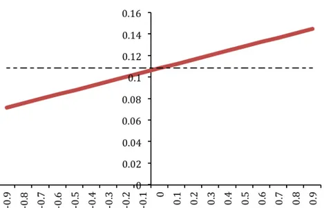
(4.3) the control selected by the controller interpreting _cω_t+1 as a time-varying intercept following a ‘return to normality’ or ‘mean reverting’ model coincides with robust control,

u0= 0.10839, when the transition parameter φ in (3.2b) is equal to 0. Alternatively the

varying intercept.

former is higher (lower) than the latter when the malevolent shocks are assumed positively (negatively) correlated. For instance for φ = 0.1 tvp-control increases to 0.11245. This is shown in Fig. 4.1 where the solid line refers to tvp-control and the dashed line to robust control.

Figure 4.1: Control at time zero determined assuming various φ’s for the ‘return to normality’ model of the time-varying intercept (solid line) vs. robust control (dashed line).

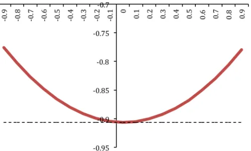
The expected costs associated with these controls, given the malevolent shocks determined by standard robust control theory (i.e. those corresponding to robust controls), are shown in Figue 4.2. In this case nature ‘doesn’t care’ about the actual control applied by the regulator in the sense that the malevolent shocks are insensitive to the φ used by the regulator assuming a time-varying intercept.33

It is apparent that the tvp control derived assuming φ = 0, i.e standard robust control, is associated with the maximum of the objective functional.

32 _{This is the parameter set originally used in MacRae (1972).}

33 _{These are the malevolent shocks associated with the robust control, i.e. ω}

Figure 4.2: Expected cost associated with controls at time zero determined assuming various φ’s for the ‘return to normality’ model of the time-varying intercept (solid line) vs. expected cost associated with standard robust control (dashed line).

When the usual malevolent shock generated by the standard robust control framework is contrasted with an hypothetically correlated malevolent control defined as34

ωt+1

H _=ρω

t + ωt+1

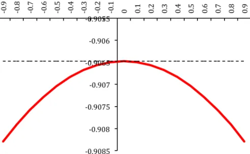
with _{ρ <}1 and the shocks _ωt and _ωt+1 as in (2.12), some interesting results emerge. As reported in Fig. 4.3 the objective functional associated with the latter reaches its minimum for ρ = 0 at a cost of −.9065.

34 _{In a problem with a longer time horizon this malevolent control may be defined as}

ωt+1 H ₌ ρω_tH _{+ ω} t+1 with ωt+1as in (2.12) and ω1 H _{≡ ω}

Figure 4.3: Expected cost associated with the control at time zero determined assuming various ρ’s for the hypothetically correlated malevolent control (solid line) vs. expected cost associated with standard robust control (dashed line).

Therefore both players optimize their objective functional by treating today’s shock (either malevolent or not) as linearly uncorrelated to tomorrow’s shock. This means that, by construction, the most common robust control framework implies that the game at time t is linearly uncorrelated with the game at time t+1.35

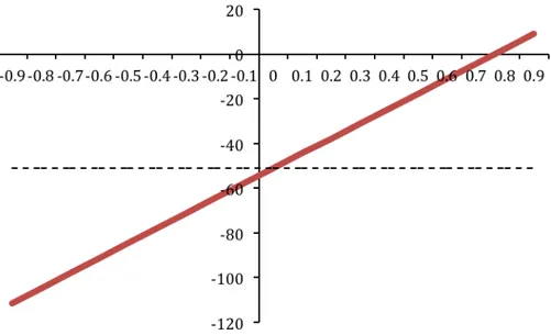
These results are not confined to the simple ‘robustized’ version of the classical MacRae (1972) problem. Indeed, exploiting Tucci’s (2009) results, they apply when unstructured uncertainty à la Hansen and Sargent is used, both in the case of a “probabilistically sophisticated” and a non-“probabilistically sophisticated” decision maker, or when uncertainty is related to unknown structural parameters of the model. For instance when the permanent income model is used, with the parameter estimates in Hansen et al. (2002),36 _both

tvp-control and robust control are equal _{−51.1 when φ = 0 but tvp-control is −57.8 when} φ = −.1, −64.5 when φ = −.2 and so on, as reported in Fig. 4.4.37

35 _{It is understood that t does not necessarily stand for calendar year. It may indicate a U.S. administration or a}

central banker term.

36 _{See, e.g., Hansen and Sargent (2001, 2003, 2007a), Hansen et al. (1999, 2002) or Tucci (2006, 2009) for a}

description of the model.

Figure 4.4: Control at time zero determined assuming various φ’s for the ‘return to normality’ model of the time-varying intercept (solid line) vs. robust control (dashed line).

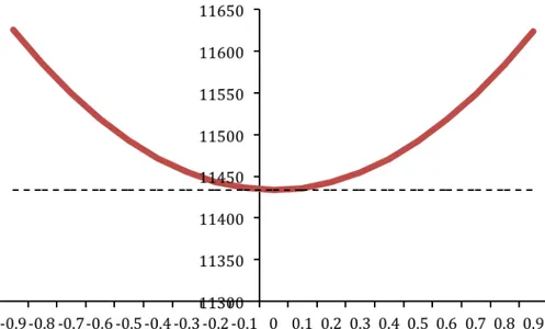
Again, the value of the objective functional associated with tvp-control is exactly the same as that for robust control, i.e. 11434, when the former uses the transition parameter φ = 0 in (3.2b) and decreases to 10874 for φ = −.1, 9193 for φ = −.2 and so on (Fig. 4.5).

Figure 4.5: Expected cost associated with controls at time zero determined assuming various φ’s for the ‘return to normality’ model of the time-varying intercept (solid line) vs. expected cost associated with standard robust control (dashed line).

As in the ‘robustized’ MacRae problem, the hypothetically correlated malevolent control attains its minimum when ρ = 0 at a cost of 11434 (Fig. 4.6).

Figure 4.6: Expected cost associated with the control at time zero determined assuming various ρ’s for the hypothetically correlated malevolent control (solid line) vs. expected cost associated with standard robust control (dashed line).

Even in this problem, widely used in robust control literature, both players (the controller and malevolent nature) optimize their objective functional by treating today’s shock (either malevolent or not) as linearly uncorrelated to tomorrow’s shock.

5. Conclusion

Tucci (2006) argues that, unless some prior information is available, the true model in a robust control setting à la Hansen and Sargent is observationally equivalent to a model with a time-varying intercept. Then he shows that, when the same “malevolent shock” is used in both procedures, the robust control for a linear system with an objective functional having desired paths for the states and controls set to zero applied by a “probabilistically sophisticated” decision maker is identical to the optimal control for a linear system with an intercept following a ‘Return to Normality’ model and the same objective functional only

when the transition matrix in the law of motion of the parameters is zero.

By explicitly taking into account the welfare loss associated with the various controls, this paper shows that the application of the usual robust control framework in discrete time problems implies that both players (the controller and malevolent nature) optimize their objective functional by treating today’s shock (either malevolent or not) as linearly uncorrelated to tomorrow’s shock. Therefore, by construction, the most common robust control framework implies that the game at time t is linearly uncorrelated with the game at time t+1. This is true not only when unstructured uncertainty à la Hansen and Sargent is used in the case of a “probabilistically sophisticated” decision maker but also, as shown in Tucci (2009), when the decision maker is non-“probabilistically sophisticated” or uncertainty is related to unknown structural parameters of the model as in Giannoni (2002, 2007).

REFERENCES

Aiyagari, S. Rao, Albert Marcet, Thomas J. Sargent and Juha Seppälä, 2002. “Optimal taxation without state-contingent debt.” Journal of Political Economy, 110(6): 1220−1254.

Barro, Robert J., 1979. “On the determination of public debt.” Journal of Political

Economy, 87(5): 940−971.

Basar, Tamer, and Pierre Bernhard, 1991. H∞-optimal control and related minimax

design problems: A dynamic game approach. Boston, MA-Basel-Berlin: Birkhäuser, 2nd Ed.

1995.

Bernhard, Pierre, 2002. “Survey of linear quadratic robust control.” Macroeconomic

Campbell, John Y., 1987. “Does saving anticipate declining labor income? An alternative test of the permanent income hypothesis.” Econometrica, 55(6): 1249−1273.

Clarida, Richard, Jordi Galì, and Mark Gertler, 1999. “The science of monetary policy: A New Keynesian perspective” Journal of Economic Literature, 37(4): 1661−1707.

Giannoni, Marc P., 2002. “Does model uncertainty justify caution? Robust optimal monetary policy in a forward-looking model.” Macroeconomic Dynamics, 6(1): 111−144.

Giannoni, Marc P., 2007. “Robust optimal policy in a forward-looking model with parameter and shock uncertainty.” Journal of Applied Econometrics 22(1): 179−213.

Hall, Robert E., 1978. “Stochastic implications of the Life cycle-Permanent income hypothesis: Theory and evidence.” Journal of Political Economy, 86(6): 971−987.

Hansen, Lars P., John Heaton and Thomas J. Sargent, 1991. “Faster methods for solving continuous time recursive linear models of dynamic economies.” In Rational

Expectations Econometrics, ed. Lars P. Hansen and Thomas J. Sargent, 177−208. Boulder, CO: Westview Press.

Hansen, Lars P. and Thomas J. Sargent, 2001. “Acknowledging misspecification in macroeconomic theory.” Review of Economic Dynamics, 4(3): 519−535.

Hansen, Lars P. and Thomas J. Sargent, 2003. “Robust control of forward-looking models.” Journal of Monetary Economics, 50(3): 581−604.

Hansen, Lars P. and Thomas J. Sargent, 2007a. Robustness. Princeton, NJ-Oxford: Princeton University Press.

Hansen, Lars P. and Thomas J. Sargent, 2007b. “Recursive robust estimation and control without commitment.” Journal of Economic Theory, 136(1): 1−27.

Hansen, Lars P. and Thomas J. Sargent, 2011. “Robustness and ambiguity in continuous time.” Journal of Economic Theory, 146 (1): 1195–1223.

Hansen, Lars P. and Thomas J. Sargent, 2016. “Sets of Models and Prices of Uncertainty. ” NBER Working Papers 22000. National Bureau of Economic Research, Inc.

Hansen, Lars P., Thomas J. Sargent and Thomas D. Tallerini, 1999. “Robust permanent income and pricing.” Review of Economic Studies, 66(4): 873−907.

Hansen, Lars P., Thomas J. Sargent and Neng E. Wang, 2002. “Robust permanent income and pricing with filtering.” Macroeconomic Dynamics, 6(1): 40−84.

Harvey, Andrew C., 1981. Time series models. Oxford: Philip Allan.

Heaton, John, 1993. “The interaction between time-nonseparable preferences and time aggregation.” Econometrica, 61(2): 353−385.

Kendrick, David A., 1981. Stochastic control for economic models. New York, NY: McGraw-Hill. Second Edition (2002) available at the Author’s web site www.eco.utexas.edu/faculty/Kendrick.

MacRae, Elizabeth C., 1972. Linear decision with experimentation. Annals of

Economic and Social Measurement, 1(4): 437–447.

Muehlen, von zur P., 1982. Activist versus non-activist monetary policy: Optimal policy rules under extreme uncertainty, reprined in Finance and Economics Discussion

Series, No 2002-02 (2001) and downloadable from www.federalreserve.gov/pubs/feds/.

Onatski, Alexei and James H. Stock, 2002. “Robust monetary policy under model uncertainty in a small model of the U.S. economy.” Macroeconomic Dynamics, 6(1): 85−110. Rotemberg, Julio J., and Michael Woodford, 1997. “An optimization-based econometric framework for the evaluation of monetary policy.” In NBER Macroeconomics

Annual 1997, ed. Ben S. Bernanke and Julio J. Rotemberg, 297−346. Cambridge, MA: MIT

Press.

Rotemberg, Julio J., and Michael Woodford, 1998. “An optimization-based econometric framework for the evaluation of monetary policy: Expanded version.” National Bureau of Economic Research Technical Working Paper 233.

Rustem, Berç, 1992. “A constrained min-max algorithm for rival models of the same economic system.” Mathematical Programming, 53(1−3): 279−295.

Rustem, Berç, 1994. “Robust min-max decisions for rival models.” In Computational

technique for econometrics and economic analysis, ed. David A. Belsley, 109−136. Dordrecht: Kluwer Academic Publishers.

Rustem, Berç, 1998. Algorithms for nonlinear programming and multiple objective

decisions. New York, NY: Wiley.

Rustem, Berç and Melendres A. Howe, 2002. Algorithms for worst-case design with

applications to risk management. Princeton, NJ: Princeton University Press.

Sims, Christopher A, 2001. “Pitfalls of a Minimax approach to model uncertainty.”

American Economic Review, 91(2): 51−54.

Tetlow, Robert and Peter von zur Muehlen, (2001a). “Simplicity versus optimality: the choice of monetary policy rules when agents must learn.” Journal of Economic Dynamics

and Control, 25(1−2): 245−279.

Tetlow, Robert and Peter von zur Muehlen, (2001b). “Robust monetary policy with misspecified models: does model uncertainty always call for attenuated policy.” Journal of

Tucci, Marco P., 2004. The rational expectation hypothesis, time-varying parameters

and adaptive control: A promising combination4. Dordrecht: Springer.

Tucci, Marco P., 2006. “Understanding the difference between robust control and optimal control in a linear discrete-time system with time-varying parameters.”

Computational Economics, 27(4): 533−558.

Tucci, Marco P., 2009. “How Robust is Robust Control in the Time Domain?”,

Quaderni del Dipartimento di Economia Politica e Statistica, 569, September.

Woodford, Michael, 1999. “Optimal monetary policy inertia.” National Bureau of Economic Research Working Paper 7261.

Woodford, Michael, 2003. Interest and prices: Foundations of a theory of monetary