Nonlinear oscillations in high power systems

Università degli Studi di Catania

Dipartimento di Ingegneria Elettrica, Elettronica e Informatica

International Ph.D. course in Systems Engineering - XXVII cycle

Ph.D. Thesis

Nonlinear oscillations in high power systems

Marco Iachello

Tutor: Prof. M. Frasca Coordinator: Prof. L. Fortuna

3

Contents

Preface ... 5

1 Introduction

1.1 Nonlinear oscillation in power electronics... 6

1.2 Nonlinear oscillation in nuclear fusion ... 10

1.2.1 Modeling plasma instabilities by using theoretical approaches ... 17

1.2.2 Modeling plasma instabilities by using experimental approaches ... 18

1.2.3 Remarks on modeling of high power systems ... 25

2 Thermal modeling of high power modules

2.1 Thermal modeling ... 27

2.2 A new integrated procedure for power electronic modules ... 29

2.3 Lumped parameter modeling ... 32

3 Identification of nonlinear oscillations in high power systems

by using neural networks

3.1 Introduction on Artificial Neural Networks (ANN). ... 40

3.2 Mathematical representation of a single neuron ... 41

3.3 Description of layer ... 43

3.4 Training ... 44

3.5 Neural network topologies ... 46

3.6 Identification of JET instabilities using neural networks... 48

3.6.1 The identification approach ... 49

3.6.2 Examples of ELM identification ... 51

4

Identification of a stable LTI plant by using a predictor and

a parallel model

4.1 Series parallel model and parallel model ... 61

4.2 Statement of the problem ... 63

4.3 Identification by using a series-parallel model (predictor) ... 63

4.4 Switching criterion ... 64

4.5 Identification by using a parallel model ... 65

4 4.7 Considerations on the applied procedure to derive the adaptive law for the parallel model . 71

5

Concluding remarks

References

5

Preface

The main topic of this work is to investigate on nonlinear phenomena affecting high power systems and on the strategies adopted to model them. In the first chapter the attention is focused on two big areas of high power systems: power electronics and systems/devices used to sustain plasma fusion. Although it is common that System Engineers tend to associate high power systems with power electronics, it is worth noting that power systems related to nuclear fusion represent a challenging area rich in nonlinearities. Specifically, while nonlinear oscillations in power electronics are due to oscillations of electrical nature, the ones present in nuclear fusion can also refer to other physical quantities. We will refer to the latter taking into account macroscopic plasma instabilities affecting JET plasmas, and proposing both theoretical approaches and experimental ones to describe their dynamic. The former rely on nonlinear mathematical equations able to mimic the nonlinear behavior of the system under certain conditions while the latter are based on a physical realization of the system starting from its mathematical model.

High power systems related to power electronics are investigated in Chapter 2 where the importance of thermal modeling for the power electronics modules is pointed out and a new modeling strategy which starts from a distributed parameter analysis to obtain a lumped parameter model is introduced.

In this case, the proposed methodology is based on the assumption that the heat transfer problem can be assumed to be linear and the thermal impedances approaches can be therefore used. In this relevant case study nonlinearities in modeling high power systems can also be neglected under certain conditions. In particular, concerning high power modules, it is well-known how the geometry of the device and the proper choice of the cooling system can play a key role for these simplifications.

A data-driven approach based on neural networks to model plasma instabilities is presented in Chapter 3. This approach is introduced because physical models often require a deep knowledge of the system parameters that sometimes is difficult to obtain.

In Chapter 4 considerations and results on new identification methodologies based on parallel identification models for discrete-time systems are presented.

6

1

Introduction

In this chapter, we will focus on two main categories of high power systems presenting nonlinear oscillations: power electronics and experimental devices for the production of fusion energy. The former is characterized by nonlinear oscillations of electrical nature while in the latter oscillations of physical quantities of different natures are also present. The insurgence of nonlinear phenomena in these fields will be discussed in order to define the framework in which different modeling and identification approaches will be discussed in this thesis.

1.1 Nonlinear oscillation in power electronics

Speaking about high power devices or systems the first field that comes to the Systems Engineer's mind is the power electronics one. Actually nonlinear oscillations are present in high power systems of different natures. Power electronics, as one of the most representative field of high power systems, is of growing importance: it is estimated that during the twenty-first century more than 90% of the electrical energy generated in developed countries will be processed by power electronics before its final consumption [1]. Power electronic systems must be energy efficient and reliable, have a high power density thus reducing their size and weight, and be low cost to make the overall system economically feasible. High energy efficiency is important for several reasons: it lowers operating costs by avoiding the cost of wasted energy, contributes less to global warming, and reduces the need for cooling therefore increasing power density.

Power electronic systems are found in virtually every electronic device: DC/DC converters are used in most mobile devices (mobile phones, PDA etc.) to maintain the voltage at a fixed value whatever the voltage level of the battery is. These converters are also used for electronic isolation and power factor correction; AC/DC converters (rectifiers) are used every time an electronic device is connected to the mains (computer, television etc.). These may simply change AC to DC or can also change the voltage level as part of their operation; AC/AC converters are used to adapt either the voltage level or the frequency (international power adapters, light dimmer). In power distribution networks AC/AC converters may be used to exchange power between utility frequency 50 Hz and 60 Hz power grids; DC/AC converters (inverters) are used primarily in UPS or renewable energy systems or emergency lighting systems. When mains power is available, it will charge the DC

7 battery. If the mains fails, an inverter will be used to produce AC electricity at mains voltage from the DC battery.

The basic module of power electronic systems is then the converter. It utilizes semiconductor devices as switches and possibly energy storage elements such as inductors and capacitors. The presence of both types of component implies that the circuits are nonlinear, time-varying dynamical systems.

There are several unavoidable sources of unwanted nonlinearity in practical power electronics circuits [1]-[3]: the semiconductor switching devices (BJTs, MOSFETs, IGBTs, thyristors, diodes) have intrinsically nonlinear DC characteristics. They also have nonlinear capacitances and inductances. The control circuits usually involves nonlinear components such as comparators, PWMs, etc.

For all these reasons power converters are intrinsically nonlinear and can exhibit a variety of complex behaviors. Bifurcation theory has been applied successfully to simple models of power systems, and it has been shown that the theory of nonlinear dynamics can be used to explain undesirable low-frequency oscillation and voltage collapses [1]. This last phenomenon occurs because many power systems are forced to operate near their stability limits and thus they are vulnerable to perturbations of the operating conditions. So when these limits are exceeded, the system can exhibit undesired transient responses with the impossibility to retain a stable voltage profile [4].

Power electronics is increasingly being used to process power on a large scale so interconnected systems of converters are developing for high current, high power applications. In order to maximize the capacity and, to reduce the cost of existing power systems as demand rises, progressive interlinking is taking place on a continental level. In this case undesirable nonlinear effects can produce catastrophic bifurcations. On the other hand nonlinear phenomena in power electronics could provide benefits. In fact, in [5] it has been demonstrated the feasibility of using chaos to depress the spectral peaks of the interference from a switched mode power supply. In particular a boost converter (operating at a low switching frequency, 2.5 kHz) has been used to show that the spectrum of the input current is spread so its peaks are reduced and EMC is improved compared to the case when the circuit operates periodically. Moreover there was the advantage that this approach did not require extra circuitry compared with other spread spectrum techniques such as pseudo-random modulation and PWM.

8 It means that one possible area of application of nonlinear phenomena in power electronics is in reducing electromagnetic interference (EMI) in switch mode power supplies which are generators of both conducted (450 kHz to 30 MHz) and radiated (30 MHz to 1GHz) EMI. Therefore suppression of EMI is a major issue in switching-mode power converter design.

The first step in order to know how and how much nonlinear phenomena in power electronics could be dangerous or could bring benefits is to understand them. In many past studies the essential method to investigate nonlinear phenomena has been to obtain a discrete-time model of the systems under study and to analyze the observed phenomena in terms of the theory of bifurcations in maps developed by mathematicians and physicists. Several studies demonstrated that, when one parameter is varied while the others are kept fixed, the system behavior could change from periodic to chaotic [6]. The inherent sensitivity of chaotic systems to small perturbations may be exploited for synchronization and stabilizing limit sets such as unstable equilibriums or periodic orbits [7]-[10]. However, applications in power electronics are less obvious, because it is already possible to force large changes in behavior by means of active switching devices. In [11] it is shown that chaotic power converters may also be stabilized by appropriate feedback. From nonlinear dynamic systems theory it is know that in most chaotic systems there are periodic windows in the parameter space and a small inadvertent change of a parameter can bring the system out of chaos. It means ask themselves the question: Are we able to ensure reliable operation of a converter under chaos? This also begs another question: is there any point in making a power converter chaotic? Hamill conjectured that power electronics converter operating under chaos instead of a stable periodic orbit may have a better dynamic response, for instance in moving rapidly from one commanded output voltage to another [12].

In this direction Banarjee, Yorke, and Grebogi developed the theory of robust chaos [10] underlining the analytical conditions under which there would be no periodic window in a chaotic system and demonstrated that such a condition does occur in current mode controlled converters. Further studies are required to attack the problem in order to make use of the chaotic regime.

The growing interest in the chaotic behaviour that power converters can exhibit led to various methods for controlling chaos developed for power electronic circuits. Poddar, Chakrabarty, and Banerjee reported experimental control of chaos in the buck converter and the boost converter [6],[13]. In [14] Marrero, Font and Verghese observed that a potential advantage of using DC-DC converters in the chaotic regime is that the switching spectrum is flattened.

9 After a reasonable understanding of the nonlinear phenomena in power electronics is obtained the main question is: can we make engineering use of them?

The above mentioned works demonstrates that research in nonlinear phenomena of power electronics is going through an important phase of development. The past years of research, characterized by engineers that observed in power devices "strange" phenomena (e.g., chaos and bifurcation), helped the scientific community to focus and approach the topic in order to give an explanation to those "bad" laboratory observations. It seems that identification work will continue to be an important area of investigation. This is because power electronics emphasizes reliability and predictability, and it is crucial to understand the system behavior as thoroughly as possible and under all kind of operating conditions. Knowing when and how a certain bifurcation occurs will automatically means, for example, how to avoid it.

10

1.2 Nonlinear oscillations in nuclear fusion

Another relevant field related to high power systems is nuclear fusion [15]. Nuclear fusion is the process powering the Sun and stars. In the core of the Sun, at temperatures of 10-15 MK, Hydrogen is converted to Helium by fusion - providing enough energy to keep the Sun burning - and to sustain life on Earth.

A vigorous world-wide research programme is underway, aimed at harnessing fusion energy to produce electricity on Earth [16]. If successful, this will offer a viable alternative energy supply within the next 30-40 years - with significant environmental, supply and safety advantages over present energy sources.

To harness fusion on Earth, different, more efficient fusion reactions than those at work in the Sun are chosen by scientists, those between the two heavy forms of Hydrogen: Deuterium (D) and Tritium (T). All forms of Hydrogen contain one proton and one electron. Protium, the common form of Hydrogen has no neutrons, Deuterium has one neutron, and Tritium has two. If forced together, the Deuterium and Tritium nuclei fuse and then break apart to form a helium nucleus (two protons and two neutrons) and an uncharged neutron. The excess energy from the fusion reaction (released because the products of the reaction are bound together in a more stable way than the reactants) is mostly contained in the free neutron.

Fusion occurs at a sufficient rate only at very high energies on earth, and temperatures greater than 100 million Kelvin are required, as shown in Figure 1.1. At these extreme temperatures, the Deuterium - Tritium (D-T) gas mixture becomes a plasma (a hot, electrically charged gas). In a plasma, the atoms become separated - electrons have been stripped from the atomic nuclei (ions). For the positively charged ions to fuse, their temperature must be sufficient to overcome their natural charge repulsion.

In order to harness fusion energy, scientists and engineers are learning how to control very high temperature plasmas. The adoption of much lower temperature plasmas are now widely used in industry, especially for semi-conductor manufacture. However, the control of high temperature fusion plasmas presents several major science and engineering challenges - how to heat a plasma to in excess of 100 MK and how to confine such a plasma, sustaining it so that the fusion reaction can become established.

11

Three parameters (plasma temperature, density and confinement time) need to be simultaneously achieved for sustained fusion to occur in a plasma. The product of these is called the fusion (or triple) product and, for D-T fusion to occur, this product has to exceed a certain quantity - derived from the so-called Lawson Criterion after British scientist John Lawson who formulated it in 1955. Attaining conditions to satisfy the Lawson criterion ensures the plasma exceeds Breakeven - the point where the fusion power out exceeds the power required to heat and sustain the plasma. Fusion reactions occur at a sufficient rate only at very high temperatures - when the positively charged plasma ions can overcome their natural repulsive forces.

Typically, in JET, over 100 MK is needed for the Deuterium-Tritium reaction to occur - other fusion reactions (e.g. D-D, D-He3) require even higher temperatures. The number of fusion reactions per unit volume is roughly proportional to the square of the density. Therefore the density of fuel ions must be sufficiently large for fusion reactions to take place at the required rate. The fusion power generated is reduced if the fuel is diluted by impurity atoms or by the accumulation of Helium ions from the fusion reaction itself. As fuel ions are burnt in the fusion process they must be replaced by new fuel and the Helium products (the "ash") must be removed. The Energy Confinement Time is a measure of how long the energy in the plasma is retained before being lost. It is defined as the ratio of the thermal energy contained in the plasma and the power input required to maintain these conditions. On JET magnetic fields are used to isolate the very hot plasmas from the relatively cold vessel walls in order to retain the energy for as long as possible. A significant

Figure 1.1: Temperature needed for plasma on Earth (>107 K)

12 fraction of losses in a magnetically-confined plasma is due to radiation. The confinement time increases dramatically with plasma size (large volumes retain heat much better than small volumes)- the ultimate example being the Sun whose energy confinement time is massive.

For sustained fusion to occur, the following plasma conditions need to be maintained (simultaneously):

 plasma temperature: (T) 100-200 MK;  energy confinement time: (t) 4-6 s;

 central density in plasma: (n) 1-2 x 1020 particles m-3 (approx. 1/1000 gm-3, i.e. one millionth of the density of air). Note that at higher plasma densities the required confinement time will be shorter but it is very challenging to achieve higher plasma densities in realistic magnetic fields.

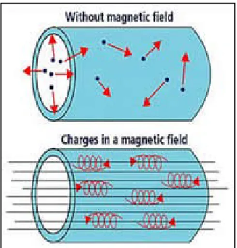
Since a plasma comprises charged particles: ions (positive) and electrons (negative), powerful magnetic fields can be used to isolate the plasma from the walls of the containment vessel - thus enabling the plasma to be heated to temperatures in excess of 100 MK. This isolation of the plasma reduces the conductive heat loss through the vessel and also minimizes the release of impurities from the vessel walls into the plasma that would contaminate and further cool the plasma by radiation. In a magnetic field the charged plasma particles are forced to spiral along the magnetic field lines (Figure 1.2).

The most promising magnetic confinement systems are toroidal (from torus: ring-shaped) and, among these, the most advanced is the Tokamak. Currently, JET is the largest Tokamak in the world although the future ITER machine will be even larger.

13 Other, non magnetic plasma confinement systems are being investigated - notably laser-induced inertial confinement fusion systems [17].

In a Tokamak the plasma is heated in a ring-shaped vessel (or torus) and kept away from the vessel walls by applied magnetic fields. The basic components of the Tokamak's magnetic confinement system are :

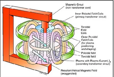
- the toroidal field - which produces a field around the torus. This is maintained by magnetic field coils surrounding the vacuum vessel (see Figure 1.3);

- the poloidal field - which produces a field around the plasma cross section. It pinches the plasma away from the walls and confines the plasma. The poloidal field is induced both internally, by the current driven in the plasma (one of the plasma heating mechanisms) and, externally, by coils that are positioned around the perimeter of the vessel.

Figure 1.3: Toroidal and poloidal coil in JET's Tokamak

The main plasma current is induced in the plasma by the action of a large transformer. A changing current in the primary winding or solenoid (a multi turn coil wound onto a large iron core in JET) induces a powerful current (up to 5 MA on JET) in the plasma - which acts as the transformer secondary circuit. A simplified cutaway diagram of JET's Tokamak is shown in Figure 1.4.

14 Figure 1.4: Simplified cutaway diagram of JET's Tokamak.

Securing future energy supply is the major challenge for Europe and the world. Global energy demand will increase over the next years as people in developing countries become wealthier. Energy sources using renewable technologies such as wind power will be necessary to satisfy future needs, but the strong energy demand leads us to develop new energy sources that can provide continuous, large-scale power for the long term without harming the environment. Fusion energy could represents a potential solution in this direction. Joint European Torus (JET), the major experiment of the European Union fusion research programme [18], has allowed studies of tokamak plasmas up to reactor relevant performance and to resolve key physics and engineering issues for the design of the International Tokamak Experimental Reactor (ITER).

Every individual plasma experiment at JET (pulse) lasts several tens of seconds and during experimental campaigns there are several pulses a day. Therefore power supplies are designed to supply pulsed loads. Each JET pulse consumes around 10GJ of energy [18]. More than 50% of this power and energy is taken by the British 400kV Grid. It means that magnetic fusion experiments require extensive use of AC/DC conversion systems: semiconductors such as diodes and thyristors must be used to convert the grid AC power into a dynamic DC form suitable for JET. (The rest of power is taken by two local flywheel generators with diode converter). A key role in the success of JET has been the development of power conversion systems, which supplies the main electrical loads of a tokamak. European countries are not the only could give a contribute to ITER development. Advanced studies in order to improve tokamaks power conversion systems are taking

15 place in other countries of the world: in China innovative power supply systems for EAST Superconducting tokamak are continually evolving and could represent a testbed for the technologies proposed for ITER project [19]. On the one hand power electronics plays, once again, a key role in JET Tokamak because nonlinear phenomena are present in tokamaks power conversion systems. On the other hand, Tokamaks are also characterized by nonlinear oscillations of different nature [15]. Specifically, tokamak plasmas are affected by a series of instabilities, which can play an important role on the performance of the plant and even compromise the correct operation of experiments. A lot of progress has been achieved in the last decades to understand the main causes of these instabilities but various aspect of their dynamics remain not completely understood. Edge Localized Modes (ELMs) are instabilities that appear when the plasma is in the high confinement mode H-mode configuration. The higher plasma energy in these configurations is partly due to a “pedestal” at the edge of the pressure profile. This pedestal results from pedestals on both the density and temperature profiles. While it is obvious that the pedestal is advantageous to achieve higher confinement, the price is paid by the inevitable steep gradients at the plasma edge which leads to instabilities – the ELMs [15].

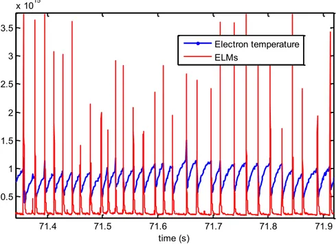
One of the main macroscopic modes in a Tokamak is the sawtooth instability which is present over a wide range of operating conditions. This is observed as a relaxation oscillation in the centre of the plasma, which appears most clearly in the time evolution of the electron temperature, derived from the Electron Cyclotron Emission on JET. The clear signature is sawtooth-like behaviour of the time series waveform in the central region of the plasma, with inverted behaviour in the outer region. The abrupt collapse of the temperature is attributed to a central, helical instability which causes the expulsion of particles and energy, detected as a heating pulse propagating in the outer region. On the plasma with high κ (density), we can observe a synchronization between ELMs and Te (electron temperature) sawteeth. When temperature collapses, an ELM can be triggered. This phenomenon is due to energy that goes from core to edge plasma. The pressure gradient becomes too important and the plasma edge loses confinement. The signature of the ELMs is very clear on the electron temperature and on the magnetic field, as measured with the pick up coils. ELMs can be also identified by Dα radiation (visible radiation emitted by excited atoms of deuterium fuel). An explicit example in Figure 1.5 shows clearly the interaction between ELMs on Dα and sawteeth on electron temperature.

16

Figure 1.5: Interaction between electron temperature (blue) sawteeth and ELMs (red) visible on Dα radiation for experiment (pulse) #50722.

There are three categories of ELMs [15]:

 Type I ELMs are essentially giant ELMs. This type is particular threat because of the large heat loss pulse involved and the consequent unacceptably high heat load on the divertor.  Type II ELMs are intermediate category which avoid the heat pulse of type I but do not lead

a severe loss of general confinement.

 Type III ELMs are continuous grassy ELMs which are associated with a substantial deterioration of confinement. 71.4 71.5 71.6 71.7 71.8 71.9 0.5 1 1.5 2 2.5 3 3.5 x 1015 time (s) Electron temperature ELMs

17

1.2.1 Modeling plasma instabilities by using theoretical approaches

Particular attention has been given to the modeling of instabilities rising evident macroscopic implications, such as ELMs, sawtooth and Neoclassical Tearing Modes. Models can be derived from experimental observations, by means of data fitting or neural networks approximations [20], or applying approaches based on geometrical consideration exploiting the peculiar characteristics of the reactor. An example of the first approach is based on neural networks for modeling ELMs and sawtooth instabilities [20], while an example of the second approach can be found in [21] where a nonlinear gross behavior model for tokamak plasmas has been introduced starting from symmetry considerations. This ideal nonlinear model is essentially based on the relatively simple application of the equivariant bifurcation theory and it is able to reproduce the principal qualitative characteristics of ohmically heated tokamak discharges. Following [21], let us consider some simplificative hypotheses on tokamak geometry. A realistic geometric approximation is to consider the tokamak as a periodic cylinder. Thanks to this simplification the simplest realistic nonlinear model satisfying rotational simmetry constraints can be described considering the generic unstable modes of amplitude with an angular coordinate φ, so that the solution may be written as:

where is the integer mode number and the denotes the complex conjugate. If the dynamics of the mode is ideal (Lagrangian), imposing invariance under rotation we obtain the following equation:

Equation can be rewritten as the following system of two first-order differential equations:

The dynamic characteristics of model (1.3) allows to mimic two important peculiarities of tokamak plasmas, i.e. the occurrence of saturated traveling waves and the bursty and sawtoothing behavior. This makes the model suitable for fitting real data acquired during experiments in which the occurrence of ELMs and sawtooth can be observed. Furthermore, quantitative information regarding the nonlinear terms in the real experiment can be useful to derive a more accurate model. An example of bursty oscillations is shown in Figure 1.6 in which the solution of the system (1.3) is obtained for initial conditions and .

18 Figure 1.6: Solutions of the system (1.3) for and initial conditions ,

.

1.2.2 Modeling plasma of instabilities by using experimental

approaches

Although the dynamics of nonlinear systems can be studied by using numerical simulations, in some cases the particular characteristics of the considered system suggest to investigate it also in presence of non ideal conditions, e.g. considering an experimental approach based on electronic analogue [22]. In fact, an electronic circuit, designed starting from the mathematical model of a dynamical system, can be easily implemented and its behavior can be characterized observing the electrical waveform generated by the circuit itself. Especially in presence of parameters which can lead to bifurcations, the behavior of the system can be more rapidly investigated with such experimental approach. The parameter values are designed applying the harmonic balance principle [23] in order to derive the conditions allowing the observation of the onset of stable nonlinear oscillations. The model introduced represents a generalization of the conservative analytical model (1.3) obtained introducing dissipative terms. The considered model is then of interest in the field of modeling physical phenomena as it represents the generalization of the plasma gross behavior model. Let us consider the following dynamical system:

0 20 40 60 80 100 120 140 160 180 200 0 0.5 1 1.5 x 0 20 40 60 80 100 120 140 160 180 200 -1 -0.5 0 0.5 1 y t

19

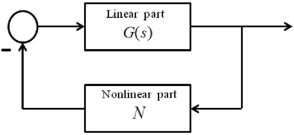
where , , and are design parameters and is a nonlinear functional. The system in Eqs (1.4) represents a nonlinear oscillator with dissipative terms and a cubic nonlinearity involving a derivative term. In order to obtain stable oscillations, system parameters can be designed following the harmonic balance approach based on the describing function (DF) approximation [24]. The analysis based on the harmonic balance method allows to identify whether or not a limit cycle is a stable solution for the considered system, provided that it has been rewritten in the so-called Lur'e form. Lur'e systems are nonlinear systems of the simplest architecture formed by a dynamical part and a feedback nonlinear part as shown in Figure 1.7.

Figure 1.7: Lur'e system block diagram.

More in detail the nonlinearity can be approximated with the corresponding static and dynamic describing function [25] and , where the amplitude and the bias of can be derived solving the equations:

where has been considered for . Solving Eqs. (1.5) means to express as a function from the static equation and the to consider the intersections between the curve and the curve in the complex plane. At each intersection corresponds a limit cycle with a given frequency, amplitude, and bias level. The stability of the predicted limit cycle can be inferred

20 applying the Loeb criterion [26]: if the points near the intersection along the curve for increasing values of are not encircled by the curve , then the limit cycle is stable. The system in Eqs (1.4) can be rewritten according to the Lur'e form as the following second-order differential equation:

where , and . The linear part of the oscillator is described by the transfer function

, while the dynamic nonlinearity can be

approximated by the following static and dynamic describing functions:

(1.7)

Substituting Eqs. (1.7) in (1.5), a unique solution can be found with

,

,

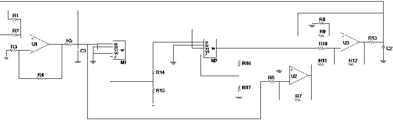
Hereinafter, the uniqueness of the limit cycle with respect to a given set of parameters will be exploited in order to design and implement a circuital analogue of the proposed oscillator. At this point, the aim of is to design a circuital implementation of the nonlinear model in Eqs. (1.4). Let us consider the circuit's schematic reported in Figure 1.8

Figure 1.8: Circuit implementing system in Eqs. (1.3)

It has been designed following the state variable approach [27], hence the circuital equations governing the circuit are:

21

OP-AMPs U1 and U3 implement an active integrator made by a passive RC group and an algebraic adder, the two cascaded multipliers M1 and M2 realize the cubic nonlinearity while OP-AMP U2 allows to set parameter . Even if the circuit is designed in order to compensate the dissipative terms involved in the integrators transfer function, dissipative effects cannot be completely avoided due to tolerances in circuital components. This means that and are small but different from zero. Furthermore, a temporal scaling has to be introduced to make signals frequency compatible with analog circuitry. We fixed

Although the nonlinear block should realize a cubic nonlinearity, the actual nonlinearity is of the form considered in Eqs. (1.4). According to [28], the model of the analog multiplier based on [29] involve further terms, in which the multiplication between the input and its derivative appears, whose coefficients are functions of the frequency of the input signal. In order to evaluate these coefficients, let us start from the assumption that the maximum signal frequency is sufficiently small, so that the higher order derivatives of the output signal can be neglected, the model of the single multiplier realizing the square term can be written as:

The parameters and can be estimated by applying a DC voltage at one of the input ports and a sinusoidal sweep signal at the other input port. Measuring the zero-frequency values of the voltage gain and the group delay relative to the AC signals using an AD633 multiplier at the time-scale of the circuit, and have been identified. Thus the model of the two cascaded multipliers is given by:

By expanding products in (1.10) and neglecting the terms the model can be rewritten as follow:

22 obtaining a value for parameter

. . The circuit parameters of

Figure 1.8 are chosen so that equations (1.8) match equations (1.2) with: , , (potentiometer), , . In this case, the values of parameters can be identified as , and . The harmonic balance method allows to determine the unique stable solution of Eqs.(1.7) as shown in Figure 1.9.

Figure 1.9. Plot of (blue line) and (black dashed line) in the complex plane for the parameter values implemented in the circuit.

The circuit, shown in Figure 1.10, has been implemented with off-the-shelf components and then analysed by acquiring the waveforms generated.

23 Figure 1.10: Circuit implementing system in Eqs. 1.3

The dataset shown in Figure 1.11 has been acquired by using a National Instruments (NI-USB6251) data acquisition board with a sampling frequency , and represents the limit cycle shown by the circuit when . Furthermore, the behavior of the circuit with respect to system parameter has been studied. According to the harmonic balance theory, the frequency of the limit cycle is directly dependent on , and, in fact, this relationship can be observed on the frequency of the limit cycle for increasing values of , as shown in Figure 1.12.

24 Figure 1.11: Limit cycle shown by the nonlinear circuit for

Figure 1.12: Frequency of the limit cycle shown by the circuit as a function of .

The model proposed above has important features which make it suitable for representing the behavior of Tokamak plasmas affected by several macroscopic and microscopic instabilities whose

0.84 0.85 0.86 0.87 0.88 0.89 0.9 0.91 1.1 1.2 1.3 1.4 1.5 1.6 1.7 1.8  fr e q u e n cy [k H z]

25 interactions are essentially nonlinear [15]. The model in Eq. (1.3) is the conservative representation of the system considered. Under this perspective, the circuital analogue presented can be used in assisting the refinement of models for the nonlinear behavior of oscillations in presence of plasma instabilities exploiting approaches based on synchronization [30].

1.2.3 Remarks on modeling of high power systems

The study discussed in the previous section underlines the importance to build the model of the high power system in order to characterize its nonlinear oscillations. More in general, the characteristics of the power devices require the definition of new identification strategies to work alongside the existing ones. According to our analysis the following emerging issues may be identified.

- The need of make use of multi-physics techniques by integrating distributed parameters modeling strategies and lumped parameter ones. Power devices have traditionally been modeled using 3D field solvers based on the finite element method (FEM). This approach, which can be described as physical modeling, entails decomposing the device/system geometry into a collection of volume or surface elements (meshing), and then solving a system of partial differential equations for the field values at the element control points. The use of multi-physics field solver allows the designer to investigate on the presence of nonlinearities of different nature. Specifically, for high power systems/modules it is of relevant importance the study of thermal aspects to ensure the reliability of the device itself that is subject to strong thermal constraints. However, often, FE modeling requires an high computational cost and for this reason the need arises to integrate it with lumped parameters modeling strategies that allow a fast simulation of the system/device. Particularly, in the thermal domain, this integration is possible by designing passive electrical networks reproducing the thermal behavior of the system/device. In Chapter 2 a new modeling methodology related to this approach has been proposed.

- The need of nonlinear models that rely on data-driven approaches to identify nonlinearities in high power systems. This is due the fact that physical models require a detailed knowledge of the device/system physics parameters that are often difficult to find. A neural network approach based on the identification of dynamical equations from data in Nuclear Fusion is presented in Chapter 3. - The need to investigate on new identification methodologies based on parallel identification models to reproduce the system behavior. Specifically the approaches based on parallel identification models are more powerful than simple series parallel identification model (predictor)

26 that require the continuous measurement of the state of the plant. In Chapter 4 an investigation on this techniques based on adaptive control is proposed.

27

2

Thermal modeling of high power modules

Power electronic modules are realized by integrating several semiconductor chips inside one package. In this chapter, a new thermal modeling procedure and its application to a power electronic module are presented [31]. The adopted modeling strategy consists of the derivation of numerical thermal impedances by 3D Finite Element (FE) models, validated by comparison with available experimental data, and of the coefficients identification of the RC passive network, through a specific topology, here introduced, to obtain a lumped parameter model of the thermal behavior of the module.

2.1 Thermal modeling

The growing demand for high power devices concentrated in small volumes is driving the industrial research towards the design of integrated power modules [32],[33]. They are realized by integrating several chips (IGBT, diodes, MOSFET) inside one package. This causes high power density that produces strong thermal constraints on the package. Furthermore, the different chips included in the device are thermally coupled, so that the thermal power generated by one chip causes the heating of both that chip and all the others in the package. Thermal aspects become dominant and strongly influence both the module working conditions and its lifetime. As a result, the probability of failure due to the thermal stress significantly increases, thus impacting on the reliability [34]-[36]. In order to keep the devices in safe operating conditions, the silicon chips junction temperature (both in transient and in steady-state regime) should be controlled. On the one hand, thermal simulators need to be more and more capable to reproduce the device thermal behavior. On the other hand, if more than just a few chips need to be thermally modeled, the simulation time of three-dimensional models increases enormously. A trade-off is therefore necessary. This study addresses the problem of reproducing the thermal behavior of high power modules by means of equivalent circuit models. Many papers describing numerical methods for thermal analyses of multichip power modules have been published [34]-[45]. Two main strategies are proposed in the literature to model the thermal behavior of a power electronic module. The first one, is a distributed parameter approach [37]-[41],[46] relying on the underlying physical mechanisms of the devices to develop a system of equations that fully describes the system response on the thermal domain. The system of equations can be solved employing different numerical methods, such as the Finite Element Method (FEM)

28 [37],[39]-[41],[46] and the Boundary Element Method (BEM)[38]. The second one, called lumped

parameters approach, reproduces the thermal behavior of the semiconductor components by deriving a thermal equivalent circuit or by using an analytical expression able to assess the thermal response of the system [42]-[44]. Both approaches lead to the derivation of thermal impedances, which represent in a concise way the thermal response of the module, at selected locations of the device. The Foster type network topology is generally proposed in the literature [42] to reproduce the behavior of both thermal self impedances and mutual impedances. Other strategies for lumped parameters modeling rely on mathematical relations to fit the thermal mutual impedance to address this problem [37].

The novelty of the proposed approach can be essentially summarized in the following points: 1) to have adopted an integrated procedure starting from FE models validated by experimental data; 2) to have introduced a new topology for the equivalent RC network used to model the thermal response of the system. The proposed topology allows to model large delays which are observed for mutual thermal impedances. The procedure is tailored on a new power module fabricated by STMicroelectronics that required a specific investigation design tool. The proposed modeling strategy consists of different steps. Firstly, a thermal 3D FE model has been derived and validated by comparison with experimental data. Then, the thermal impedances extracted from the FE model, have been reproduced by means of passive circuit topologies whose parameters are identified using optimization algorithms. Thermal data, collected by measurements or FE simulations, can be used for modeling in an electrical circuit simulator, if an electrical equivalent network whose step response describes the transient thermal impedance is available. Although the idea of finite element analysis and equivalent circuits is not new, the typical passive network topologies used to address this problem (Foster and Cauer networks) have significant limitations in accurately representing thermal mutual impedances. In this paper an electrical passive network topology is presented to emulate the transient mutual impedances which are characterized by slow transients. More specifically, the relevant quantity used to estimate the transfer function is the temperature response from the output port of the equivalent circuit. As explained in Section 2.3, thermal mutual impedances are often characterized by a time delay depending on the chips mutual position inside the package. The proposed passive network topology is able to properly reproduce both the thermal impedances transient behavior and their steady state regime.

29

2.2 A new integrated procedure for power electronic modules

The methodology introduced to characterize the thermal behavior of a power module consists of different steps shown in Figure 2.1. The first step is to collect thermal data. Thermal impedances waveform can be obtained from both a FE model or experimental data (FE Model/Experimental Characterization). The FE model allows to obtain the spatial distribution of temperature, while experimental data are usually related to temperature information at some critical points (Thermal Data). Once thermal impedances are available, the next step of the procedure is the choice of the model. In particular, the model structure is fixed (as discussed in Section III), while the order N of the system has to be selected. This step is indicated as choice of the RC equivalent model. The circuit parameters are identified by using optimization techniques based on the Nelder-Mead simplex method which minimizes the error between the thermal impedance provided by the network and the one extracted from the FE model or from experimental data (Parameters Identification). At this point it is possible to check whether the chosen order N of the equivalent RC network suffices to properly fit the thermal impedances (Validation stage). If the order N is not able to ensure a good fit, the procedure steps back to the choice of the order of the equivalent RC model. The last step of the developed procedure consists of performing the fast simulation of the whole module thermal behavior by means of a generic circuit simulator (Fast Simulation of thermal behavior). As mentioned above, two different approaches may be adopted to extract the thermal behavior of the module. In the proposed approach, thermal data have been generated by numerical models built-up exploiting the COMSOL Multiphysics software, a commercial FE-based software able to solve both partial and ordinary differential equations.

30 Figure 2.1: Flow Diagram of the proposed methodology.

The heat conduction equation describing the temperature field in the computational domains is [47]:

where represents the temperature, the thermal diffusivity, is the thermal conductivity and the volumetric heat generation. Eq (2.1) is solved by using the FE method, mainly consisting in the discretization of the continuous equations on the physical computational domains by means of chosen numerical elementary entities, i.e. the finite elements. This step allows the partial differential equation to turn into an algebraic system of equations, which is solved applying the unsymmetric multifrontal package direct solver [48]. Once initial and boundary conditions are

assigned, the solution can be computed and gathered in terms of temperature distribution all over the module. Typically, power modules are made by thin vertical layers and have large horizontal dimensions. It means that the heat flux predominantly flows from the top to the bottom of the module. Therefore, the flux through the lateral sides can be neglected, and adiabatic constraint can be assumed as the boundary condition. A properly designed heat sink allows to dissipate the whole

31 heat generated; then, the baseplate’s bottom side can be assumed as an isothermal surface. In these conditions the heat transfer problem can be assumed to be linear [37],[45] and this approximation finds good agreement with most of the power electronic applications. Under this hypothesis, the superposition principle can be used. The thermal behavior of the module may be therefore obtained by assuming, at each time, only one device acting as a heat source and evaluating the temperature along the module. The procedure is then repeated for each device of the module and the results added to obtain the complete thermal response. In particular, a power pulse ( ) is applied only on a single chip and then the thermal responses on all chips are obtained. The temperature of the bottom side of the baseplate is called reference temperature ( ). The approach is schematically shown in Figure 2.2. More specifically, the input power is applied as a surface power density uniformly distributed on the chip top surface equivalent to a power of . The reference temperature is .

Figure 2.2: Approach used to evaluate thermal responses on the different chips of the module.

To characterize the thermal response of all chips, the generic thermal impedance is defined as:

(2.2)

where is the power applied on chip j and is the temperature on the centre of the chip i top area, when chip j is heated. If the response is named thermal self impedance while if the resulting is named thermal mutual impedance and represents the thermal coupling effect between the two considered devices. Then, for a module having n devices, it is possible to assemble the following matrix of thermal impedances:

32

in which the entries in the main diagonal are the self impedances of each chip while the other terms are the mutual impedances describing the coupling effects between chips.

Combining equations (2.2) and (2.3), the complete model can be written in matrix-form as:

where is the thermal impedances matrix,

P

P=[P

, P

, …, P

]

=[T

-T

, T

-T

,…,T

-T

]

between the temperature chip and the reference temperature .

2.3 Lumped parameter modeling

The thermal data extracted by the FE model are used to derive an equivalent RC network. This is possible thanks to the analogy between thermal and electrical quantities as reported in Table I.

TABLE I:

Analogy between thermal and electrical quantities. Thermal power Electrical current Temperature difference Voltage difference

Thermal capacity Electrical capacity Thermal resistance Electrical resistance

The aforementioned analogy leads to a wide use of RC passive circuits topologies to reproduce the thermal behavior of a power device [43]. The typical passive topology used to estimate the junction temperature of a chip is the RC Foster network [42] shown in Figure 2.3a. The junction temperature estimation (and consequently the linearly related thermal impedance) is given from the voltage drop across the input port. Nevertheless, the use of RC Foster networks for the reproduction of the thermal impedances is not always suitable. In fact, we have found that this approach works well to reproduce the thermal self impedance behavior but is not able to fit properly the mutual impedance.

33 The reason of this is related to the delay characterizing thermal mutual impedances as underlined in Section 2.4. This delay increases when the distance between chips grows.

In [37], another strategy to address the reproduction of thermal mutual impedances behavior is based on the use of mathematical relations. The approach proposed in this paper deals with this problem in the framework of passive networks by defining adequate topologies for the two cases of self and mutual impedances. Specifically, the Foster type network of Figure 2.3a is used to reproduce the self impedances behavior, while thermal mutual impedances are modeled by means of the circuit topology of Figure 2.3b.

Pin T _{C1 C2 C3 CN} R1 R2 R3 RN (a) R R1 R2 R3 RN C1 C2 C3 T CN Pin (b)

Figure 2.3: RC passive networks: a) Foster RC-network for thermal self impedance; b) RC-network for thermal mutual impedance.

By comparing the circuit of Figure 2.3a with the circuit of Figure 2.3b it is possible to point out that the temperature used to calculate the thermal impedances is evaluated at different network points. In fact, in the circuit of Figure 2.3b the output is evaluated as the voltage drop across CN. In the case of

mutual impedance the temperature of the device changes as the result of heating the device j, and heat transfer occurs through several layers (involving different thermal capacity-resistance terms). This topology, as shown in Section 2.4, allows to fit properly the transient part of the mutual impedances.

The transfer function for the RC Foster type network ( Figure 2.3a ) is:

34 while the transfer function of the RC network used for the thermal mutual impedances reproduction (Figure 2.3b) is obtained by following the procedure described in [49],[50]. Specifically, let us define the transfer function for each cell (RC group) composing the circuit of Figure 2.3b as

while for the first cell made only of the resistor R, it holds:

Let indicate with and the input and output electrical impedance of the k-th cell:

Let us further introduce the quantities:

35 Then, from equations (2.10) through equations (2.6)-(2.9) the transfer function of the RC circuit in Figure 2.3b is:

The unit step response functions of circuits 3a and 3b describe the self thermal impedance and the mutual thermal impedance, respectively.

The form of these step response functions motivates the choice of the topology in Figure 2.3b. Typically, thermal mutual impedances show a quite slow transient due the horizontal heat propagation through the layers of the module. In mathematical terms this is expressed by the fact that the Taylor expansion around t = 0 of the thermal response z(t), that is

needs to have small coefficients _{(z(0)=0 as it starts from zero initial conditions).}

In particular, the network of Figure 2.3b allows to obtain a step response function having all coefficients _{exactly equal to zero, thus facilitating to match the slow transient}

shown by FE results. In the following we relate the coefficients in the Taylor expansion of the step response function (2.12) with the coefficients of the transfer function of the networks of Figure 2.3a and 2.3b.

Let be the transfer functions

Let us indicate with the unit step response of the two types of networks. Then, the initial value theorem can be used to estimate the coefficient . In fact, it holds under the hypothesis of zero initial conditions :

36 We notice that for the network of Figure 2.3a, being a positive real function, . In fact, the circuit of Figure 2.3a is a relaxation system [58] with alternated finite zeros and poles and positive residues. Thus, the relative degree of this transfer function is always equal to one. This implies that in a neighborhood of the time origin the step response of the network will have a positive slope. On the contrary, for the network of Figure 2.3b we show that , implying that the step response will start with a null slope. Furthermore, , nullifying the corresponding contribution of the high-order Taylor terms to the growth of the network step response. In fact, when , for network of Figure 2.3b, we can calculate _as:

And with an analog procedure also the high order coefficients

are found to be zero for the network of Figure 2.3b. In fact, the Ladder network with the capacitors configuration as in Figure 2.3b is a low-pass filter with a transfer function having no finite zeros [59]. As an example we consider the identification of a thermal self impedance and a mutual one [31]. In particular we consider and . We have

where the transfer functions have been obtained with the values specified in Table I. It is evident that has no finite zeros and is characterized by a relative degree four while , having three zeros, is characterized by a relative degree one.

The unit step response of and is shown in Figure 2.4. In contrast to the thermal self impedance behavior, the mutual impedances are affected by a delay related to the distance between chips. Moreover, as underlined in the case study proposed in [31], it is possible to observe that the higher is the distance between chips, the higher will be the delay and the smaller will be the thermal coupling described by the thermal mutual impedances.

37 Figure 2.4: a) Unit step response of ; b)Unit step response of ;

TABLE I: RC NETWORK PARAMETERS [°C/W] [°C/W] [°C/W] [°C/W] R [Ω] - 0.0294 0.0107 0.0024 R1 [Ω] 0.0114 0.0042 0.0015 0.0104 C1 [F] 0.0046 0.4816 2.3097 3.3168 R2 [Ω] 0.0727 0.3024 0.0040 0.2610 C2 [F] 0.1108 0.0478 1.8722 0.1656 R3 [Ω] 0.0249 1.1730 0.0639 4.3448 C3 [F] 0.0134 0.0002 0.4014 0.0087 R4 [Ω] 0.1888 0.2338 0.9098 54.6838 C4 [F] 0.2243 0.0362 0.0374 0.0008

To identify the model parameters R and C of equations (2.5) and (2.11) the Nelder-Mead simplex optimization method [51], [52] is used. The parameters identification was performed by comparison of the thermal impedance provided by the FE simulations, zFE(t), with the unit step response, zRC(t),

of the systems described by equations (2.5) and (2.11).

100 -4 10-3 10-2 10-1 100 0.1 0.2 0.3 (a) z 21 [° C /W ] 100 -4 10-3 10-2 10-1 100 0.01 0.02 0.03 Time [s] (b) z 11 [° C /W ]

38 More specifically, the objective function to be minimized takes into account the error

between the two impedances and their time derivatives:

in which the first term is the Euclidean norm of the error between zRC and zFE while the second term

is the Euclidean norm of their time derivatives and τ is the observation time. In our work we fixed

τ =10s. Equation (2.16) is a multi objective function that takes into account the error in both the

impedances and their time derivatives estimates (with _{). It is worth noticing that the first}

term of equation (2.16) is not able to ensure a good fit of the transient part of the impedance, characterized by a relevant slope. For such a reason the second term, based on the impedance time derivatives, has been introduced. The proposed approach can be used to properly reproduce all self and mutual impedances and then to describe the whole module thermal behavior. Thanks to the system linearity, the superposition principle can be applied and the thermal impedances extracted from circuits can be added according to equation (2.4). This means that by combining all derived RC circuits, as shown in Figure 2.5, it is possible to simulate in a fast and efficient way the module thermal behavior by means of a generic circuit simulator. Eventually, data acquired by using an experimental setup are used to validate the approach against real data.

+ + + + + + + + + + + + Z11 Z12 Z13 Z23 Z21 Z22 Z31 Z32 Z33 Pin T C1 C2 C3 CN R1 R2 R3 RN Pin T _{C1 C2 C3} CN R1 R2 R3 RN Pin T C1 C2 C3 CN R1 R2 R3 RN R R1 R2 R3 RN C1 C2 C3 T CN Pin R R1 R2 R3 RN C1 C2 C3 T CN Pin R R1 R2 R3 RN C1 C2 C3 T CN Pin R R1 R2 R3 RN C1 C2 C3 T CN Pin R R1 R2 R3 RN C1 C2 C3 T CN Pin R R1 R2 R3 RN C1 C2 C3 T CN Pin

39 The approach proposed in this thesis is general as it can be used to extract the thermal networks either from FE models or experimental data of thermal impedances. Furthermore, the number of variables in the model is reduced by starting from physical considerations enabling the identification of the points to be used to build the model, that is, for instance, the temperatures of selected locations of the module (IGBTs and diodes). Finally, the order of the obtained model is typically low. The aforementioned methodology has been applied successfully for a case of study proposed in [31].

40

3

Identification of nonlinear oscillations in high power systems by using

neural networks

In this Chapter a brief presentation of the use of neural networks to identify nonlinear oscillations in JET plasmas in [20] and [60] is introduced. Then, the methodology used to predict JET instabilities is discussed in detail.

3.1 Introduction on Artificial Neural Networks (ANN)

Artificial neural networks (ANN) are mathematical models, inspired by the structure of biological neural networks, made up of elementary units called neurons which are able to perform simple computations [61], [62]. They are used to solve classification and nonlinear functions approximation problems. One of the neural network features is to be inspired to the structure of the human brain, taking advantage from the main feature, the ability to learn from experience. Neural networks require a training phase using examples to acquire the experience necessary to provide the correct output in the face of new inputs.

Advantages:

 A neural network can perform tasks that a linear program cannot.

 When an element of the neural network fails, it can continue without major problems by their parallel nature.

 A neural network learns and does not need to be reprogrammed.  It can be implemented in any application.

 It can be implemented easily.

Disadvantages:

 The neural network needs training to operate.

 The architecture of a neural network is different from the architecture of microprocessors therefore needs to be emulated.

41  Requires high processing time for large neural networks.

Artificial neural networks (ANNs) are among the most attractive signal processing technologies in the engineer's toolbox [61]. The field is highly interdisciplinary, but our approach will restrict the view to the engineering perspective. In engineering we can define an artificial neural network as an adaptive, most often nonlinear system, that learns to perform a function, an input/output map, from data. Adaptive means that the system parameters are changed during operation, normally called the training phase. After the training phase the ANN parameters are fixed and the system is deployed to solve the problem at hand in testing phase. The input/output data are fundamental in neural network technology, because they convey the necessary information to discover the optimal operating point. The nonlinear nature of the neural network processing elements provides the system with lots of flexibility to achieve practically any desired input/output map, so some ANNs are universal approximators [64], [65].

3.2 Mathematical representation of a single neuron

Let us consider an ANN as a computational system densely connected that is able to store knowledge by means of experiments. The acquired knowledge is stored using the values of some parameters, called weights, which connect the computational units, called neurons, whose values are fixed during the training phase. Each neuron is an entity that has multiple inputs and one output, so is a MISO (Multi input single output) system [62]. It receives inputs from neighboring neurons, processes them and sends the output to other neurons weighing it appropriately. The currently most widely used neuron model is shown in Figure 3.1 where is the i-th input, is the weight of the

i-th input and is a function, usually non linear, called activation function. The neuron has a bias which is added to the inputs weighted sum with a unit weight. The sum

is called net input. The output of the neuron is the value of the activation function at the net input.

42 Figure 3.1: Artificial neuron.

The output of the neuron is then given by the formula:

Each neuron can use different activation functions to generate its own output. Let us consider, as shown in figures Figure 3.2 that a is the neuron's output while n is the net input.

(a) (b) (c) (d)

Figure 3.2: Activation functions of an ANN: (a) hard limit, (b) linear, (c) sigmoid, (d) hyperbolic tangent.

43

3.3 Description of layers

As shown on Figure 3.3, a layer [61]-[65] consists of S neurons working in parallel. Each unit performs a relatively simple job: it receives input from neighbors or external sources and uses this to compute an output signal which is propagated to other units. All neurons take their inputs from the same input vector (containing R inputs). If the layers have S neurons, then the layer output will be a S sized vector. As a result, the weight matrix W is an SxR sized matrix, the bias vector b and the output vector a are vectors containing S elements.

Figure 3.3: A hard limit neural layer. Left: detailed architecture of a neural layer. Right: compressed notation of a neural layer.

Each neuron of the same layer has the same activation function f. We can write the layer output vector, , as a product of matrices:

where

44

in fact the output of the j-th neuron is calculated as:

3.4 Training

Before using a neural network, weights and biases have to be adjusted [61]. Training is a process, to adjust the network coefficients, that requires a set of examples of proper network behavior. The training process is performed by means of learning algorithms which depend on the kind of network used. There are several learning approaches each corresponding to a particular abstract learning task. These are supervised learning and unsupervised learning.

The learning algorithms are called supervised when, during the training, we apply to the network an input-output dataset. The objective is to determine an adaptive algorithm or rule which adjusts the parameters of the network based on a given set of input-output pairs. If the weights of the network are considered as elements of a parameter vector ϑ, the learning process involves the determination of the vector which optimizes a performance function based on the output error. The simplest method used for this purpose is back propagation [65] in which the gradient of the performance function with respect to ϑ is computed as and ϑ is adjusted along the negative gradient as

where , the step size, is a suitably chosen constant and denotes the nominal value of at which the gradient is computed.

The weights and biases of the network are then iteratively adjusted to minimize performance function that is typically the mean square error between the network outputs and the target outputs. When the training begins, initial weights and biases are initialised randomly. This haphazard initial conditions permit to avoid falling always in the same local minima of a function. The training method is based on gradient descent therefore, the network can fall in an error local minimum if it always starts from the same initial weights.