LARGE-SCALE SIMULTANEOUS INFERENCE WITH APPLICATIONS TO THE DETECTION OF DIFFERENTIAL EXPRESSION
WITH MICROARRAY DATA G.J. McLachlan, K. Wang, S.K. Ng
1. INTRODUCTION
Often the first step, and indeed the major goal for many microarray studies, is the detection of genes that are differentially expressed in a known number of classes, C1, ..., Cg. Statistical significance of differential expression can be tested by
performing a test for each gene. When many hypotheses are tested, the probabil-ity that a type I error (a false positive error) is committed increases sharply with the number of hypotheses. In this paper, we focus on the use of a two-component mixture model to handle the multiplicity issue, as proposed initially by McLachlan, Bean, and Ben-Tovim Jones (2006). This model is becoming more widely adopted in the context of microarrays, where one component density cor-responds to that of the test statistics for genes that are not differentially ex-pressed, and the other component density to that of the test statistic for genes that are differentially expressed. For the adopted test statistic, its values are trans-formed to z-scores, whose null and non-null distributions can be represented by a single normal each. We explain how this two-component normal mixture model can be fitted very quickly via the EM algorithm started from a point that is
com-pletely determined by an initial specification of the proportion π0 of genes that are
not differentially expressed. There is an easy to apply procedure for determining suitable initial values forπ0 in the case where the null density is taken to be
stan-dard normal (the theoretical null distribution). We also consider the provision of an initial partition of the genes into two groups for the application of the EM
al-gorithm in the case where the adoption of the theoretical null distribution would appear not to be appropriate and an empirical null distribution needs to be used. We demonstrate the approach on a data set that has been analyzed previously in the bioinformatics literature.
In the above formulation of the problem, it is assumed that there is a nonzero proportion of the genes that are differentially expressed. We shall consider also an example where there would appear to be no differentially expressed genes. Hence it is advised in general that one should in the first instance carry out a test
of a single normal distribution versus a mixture of two normal components; that is, a test of an empirical null only versus a mixture of an empirical null and non-null normal component.
2. BACKGROUND 2.1. Notation
Although biological experiments vary considerably in their design, the data generated by microarrays can be viewed as a matrix of expression levels. For m microarray expreriments (corresponding to m tissue samples), where we measure the expression levels of N genes in each experiment, the results can be repre-sented by N × m matrix. Typically, m is no more than 100 (usually much less in the present context), while the number of genes N is of the order of 104 . The m
tissue samples on the N available genes are classified with respect to g different classes, and it is assumed that the (logged) expression levels have been preproc-essed with adjustment for array effects.
2.2. Detection of differential expressions
Differential expression of a gene means that the (class-conditional) distribution of its expression levels is not the same for all g classes. These distributions can differ in any possible way, but the statistics usually adopted are designed to be sensitive to primarily a difference in the means; for example, the oneway analysis of variance (ANOVA) F-statistic. Even so, the gene hypotheses being tested are of
equality of distributions across the g classes, which allows the use of permutation methods to estimate P-values if necessary.
In the special case of g = 2 classes, the oneway ANOVA F-statistic reduces to the square of the classical (pooled) t-statistic. Various refinements of the t-statistic have been suggested; see, for example, the procedure of Tusher et al. (2001).
3. TWO-COMPONENT MIXTURE MODEL
3.1. Posterior probability of nondifferential expression
In this paper, we focus on a decision-theoretic approach to the problem of finding genes that are differentially expressed, as proposed in McLachlan, Bean, and Ben-Tovim Jones (2006). Their approach is based on a two-component mix-ture model as formulated in Lee et al. (2000) and Efron et al. (2001). We let G de-note the population of genes under consideration. It can be decomposed into two groups G0 and G1, where G0 is the group of genes that are not differentially
ex-pressed, and G1 is the complement of G0; that is, G1 contains the genes that are
differentially expressed. We let πi denote the prior probability of a gene belonging
gene j in Gi is fi(wj). The unconditional density of Wj is then given by the
two-component mixture model,
f (wj) = π0 f0(wj) + π1 f1(wj ) (1)
Using Bayes Theorem, the posterior probability that the jth gene is not differ-entially expressed (that is, belongs to G0 ) is given by
τ0(wj) = π0 f0(wj )/f (wj ) ( j= 1, ..., N ). (2)
In this framework, the gene-specific posterior probabilities provide the basis for optimal statistical inference about differential expression. The posterior prob-ability τ0(wj) has been termed the local false discovery rate (local FDR) by Efron
and Tibshirani (2002). It quantifies the gene-specific evidence for each gene. As noted by Efron (2004), it can be viewed as an empirical Bayes version of the Ben-jamini-Hochberg (1995) methodology, using densities rather than tail areas.
It can be seen from (2) that in order to use this posterior probability of nondif-ferential expression in practice, we need to be able to estimate π0, the mixture
density f(wj), and the null density f0(wj), or equivalently, the ratio of densities f0(wj)/f (wj). Efron et al. (2001) has developed a simple empirical Bayes approach
to this problem with minimal assumptions. This problem has been studied since under more specific assumptions, including the work by Newton et al. (2001, 2004), Lönnstedt and Speed (2002), Pan et al. (2002), Zhao and Pan (2003), Broët
et al. (2004), Newton et al. (2004), Smyth (2004), Do et al. (2005), and Gottardo et al. (2006), among many others. The fully parametric methods that have been
pro-posed are computationally intensive.
3.2. Bayes decision rule
Let e01 and e10 denote the two errors when a rule is used to assign a gene as
be-ing differentially expressed or not, where e01 is the probability of a false positive
and e10 is the probability of a false negative. That is, the sensitivity is 1 - e10 and
the specificity is 1 - e01. The so-called risk of allocation is given by
Risk = (1 – c )π0e01 + cπ1e10, (3)
where (1 - c) is the cost of a false positive. As the risk depends only on the ratio of the costs of misallocation, they have been scaled to add to one without loss of generality.
The Bayes rule, which is the rule that minimizes the risk (3), assigns a gene to
G1 if τ0 (wj ) ≤ c; otherwise, the jth gene is assigned to G0.
4. SELECTION OF GENES
In practice, we do not know the prior probability π0 nor the densities f0(wj) and f (wj), which will have to be estimated. We shall shortly discuss a simple and quick
approach to the estimation problem. If π , f w , ˆ0 ˆ0( j) and (f w ˆ1 j) denote estimates
of π0, f0(wj), and f1(wj), respectively, the gene-specific summaries of differential
ex-pression can be expressed in terms of the estimated posterior probabilities
0 ˆ ( j) τ w , where 0 0 0ˆ ˆ ˆ ( j) ˆ ( j)/ ( j) ( 1,..., ) τ w = π f w f w j = N (4)
is the estimated posterior probability that the jth gene is not differentially ex-pressed. An optimal ranking of the genes can therefore be obtained by ranking the genes according to the τ w ranked from smallest to largest. A short list of ˆ (0 j)
genes can be obtained by including all genes with τ w less than some thresh-ˆ (0 j)
old c0 or by taking the top N0 genes in the ranked list.
4.1. FDR
Suppose that we select all genes with
0 0
ˆ ( j)
π w ≤ c . (5)
Then McLachlan et al. (2004) have proposed that the false discovery rate (FDR) of
Benjamini-Hochberg (1995) can be estimated as
n 0 0 [ 0, ] 0 1 ˆ ˆ FDR (N j) c ( ( j))/ r j = τ w I τ w N =
∑
, (6)where Nr is the number of selected genes and IA (x) is the indicator function,
which is one if x ∈ A and is the zero otherwise.
Similarly, the false nondiscovery rate (FNDR) can be estimated by
n 1 [0 ] 0 1 ˆ ˆ FNDR (N j) c , ( ( j))/( r) j = τ w I ∞ τ w N N = −
∑
. (7)We can also estimate the false positive rate (FPR), e01, and the false negative
(FNR), e10, in a similar manner to give
n 0 0 [0 ] 0 0 1 1 ˆ ˆ ˆ FPR (N j) , c ( ( j))/ N ( j) j j = τ w I τ w τ w = =
∑
∑
(8) and n 0 1 ( ) 0 1 1 1 ˆ( ) ( (ˆ ))/ ˆ( ) N N j c , j j j j FNR = τ w I ∞ τ w τ w = =∑
∑
(9) respectively.When controlling the FDR,it is important to have a guide to the value of the
associated FNR in particular, as setting the FDR too low may result in too many
false negatives in situations where the genes of interest (related to the biological pathway or target drug) are not necessarily the top ranked genes; see, for example, Pawitan et al. (2005). The local FDR in the form of the posterior probability of nondifferential expression of a gene has an advantage over the global measure of
FDR in interpreting the data for an individual gene; see more details in Efron (2005b).
5. USE OF Z-SCORES 5.1. Normal transformation
We let Wj denote the test statistic for the test of the null hypothesis
Hj : jth gene is the not differentially expressed. (10)
For example, as discussed above, Wj might be the t- or F-statistic, depending on
whether there are two or multiple classes. Whatever the test statistic, we follow McLachlan et al. (2006) and proceed in a similar manner as in Efron (2004) to transform the observed value of the test statistic to a z-score given by
zj = Ф-1(1 – Pj ), (11)
where Pj is the P-value for the value wj of the original test statistic Wj and Ф is the N(0, 1) distribution function. Thus
Pj = 1 – F0(wj) + F0(-wj), (12)
where F0 is the null distribution of Wj . If F0 is the true null distribution, then the
null distribution of the test statistic Zj corresponding to zj is exactly standard
normal. With this definition of zj, departures from the null are indicated by large
positive values of zj. The transformation (11) is slightly different to that in Efron
(2004), as we wish that only large positive values of the z-score be consistent with the alternative hypothesis; that is, we want the latter to be (upper) one-sided so that the non-null distribution of the z-score can be represented by a single normal distribution rather than a mixture in equal proportions of two normal compo-nents with means of opposite sign. Previously, Allison et al. (2002) had considered mixture modelling of the P-values directly in terms of a mixture of beta distribu-tions with the uniform (0,1) distribution (a special form of a beta distribution) as the null component. Pounds and Morris (2003) considered a less flexible beta mixture model for the P-values, being a mixture of a uniform (0,1) distribution for the null and a single beta distribution for the non-null component. In the work of Broët et al. (2004), they used a transformation similar to the approxima-tion of Wilson and Hilferty (1931) for the chi-squared distribuapproxima-tion to transform the value Fj for the F-statistic for the jth gene to an approximate z-score.
5.2. Permutation assessment of p-value
In cases where we are unwilling to assume the null distribution F0 of the
origi-nal test statistic Wj for use in our normal transformation (11), we can obtain an
assessment of the P-value Pj via permutation methods. We can use just
permuta-tions of the class labels for the gene-specific statistic Wj. This suffers from a
granularity problem, since it estimates the P-value with a resolution of only 1/B, where B is the number of the permutations. Hence it is common to pool over all
N genes. The drawback of pooling the null statistics across the genes to assess the
null distribution of Wj is that one is using different distributions unless all the null
hypotheses Hj are true. The distribution of the null values of the differentially
ex-pressed genes is different from that of the truly null genes, and so the tails of the true null distribution of the test statistic is overestimated, leading to conservative inferences; see, for example, Pan (2003), Guo and Pan (2005), and Xie et al. (2005).
6. TWO-COMPONENT NORMAL MIXTURE
By working in terms of thezj-scores as defined by (11), we can provide a
para-metric version of the two-component mixture model (1) that is easy to fit (McLachlan et al., 2006). The density of the test statistic Zj corresponding to the
use of the z-score (11) for the jth gene is to be represented by the two-component normal mixture model
f (zj) = π0f0(zj ) + π1f1(zj ), (13)
where π1 = 1 - π0 . In (13), f0(zj ) = φ(zj ; 0, 1) is the (theoretical) null density of Zj,
where φ(z ; µ, σ2 ) denotes the normal density with mean µ and variance σ2, and
f1(zj) is the non-null density of Zj. It can be approximated with arbitrary accuracy
by taking q sufficiently large in the normal mixture representation
2 1 1 1 1 1 ( ) π ( ; , ) q j h j h h h f z =
∑
φ z µ σ = . (14)For the data sets that we have analysed, it has been sufficient to use just a single normal component (q = 1) in (14). In such cases, we can write (13) as
2
0 1 1 1
( )j ( ; 0 ,1)+ j ( ; ,j )
f z = π φ z π φ z µ σ . (15)
As pointed out in a series of papers by Efron (2004, 2005a, 2005b), for some microarray data sets the normal scores do not appear to have the theoretical null distribution, which is the standard normal. In this case, Efron has considered the estimation of the actual null distribution called the empirical null as distinct from the theoretical null. As explained in Efron (2005b), the two-component mixture
model (1) assumes two classes, null and non-null, whereas in reality the differ-ences between the genes range smoothly from zero or near zero to very large.
In the case where the theoretical null distribution does not appear to be valid and the use of an empirical null distribution would seem appropriate, we shall adopt the two-component mixture model obtained by replacing the standard normal density by a normal with mean µ0 and variance σ02 to be inferred from
the data. That is, the density of the zj-score is modelled as
2 2
0 0 0 1 1 1
( )j ( ; j , )+ ( ; ,j )
f z = π φ z µ σ π φ z µ σ (16)
In the sequel, we shall model the density of the zj-score by (16). In the case of
the theoretical N(0, 1) null being adopted, we shall set µ0 = 0 and σ02= 1 in (16).
7. FITTING OF NORMAL MIXTURE MODEL 7.1. Theoretical null
We now describe the fitting of the two-component mixture model (15) to the
zj , firstly with the theoretical N(0, 1) null adopted. In order to fit the
two-component normal mixture (15), we need to be able to estimate π0 , µ1 , and σ12.
This is effected by maximum likelihood via the EM algorithm of Dempster et al.
(1977), using the EMMIX program as described in McLachlan and Peel (2000); see
also McLachlan and Krishnan (1997). To provide a suitable starting value for the
EM algorithm in this task, it is noted that the maximum likelilhood (ML)estimate
of the parameters in a two-component mixture model satisfies the moment equa-tions obtained by equating the sample mean and variance of the mixture to their population counterparts, which gives
0 0ˆ 1 1ˆ ˆ ˆ = z π µ +π µ (17) and 2 2 2 0ˆ0 1ˆ1 0 1 ˆ0 ˆ1 ˆ ˆ ˆ ˆ ( ) 2 z s = π σ +π σ +π π µ −µ , (18)
where π = - π . For the theoretical null, ˆ1 1 ˆ0 µˆ0= and 0 σ02= and on substitut-1
ing for them in (17) and (18), we obtain
1 0 ˆ z/(1-πˆ ) µ = (19) and 2 2 2 1 0 0 0 1 0 ˆ {sz πˆ πˆ (1 πˆ ) } (1ˆ / πˆ ) σ = − − − µ − . (20)
Hence with the specification of an initial value (0) 0
π for π0, initial values for the
other parameters to be estimated, µ1 and σ12, are automatically obtained from (19)
and (20). If there is a problem in so finding a suitable solution for µ1(0) and
2
(0) 1
σ , it gives a clue that perhaps the theoretical null is inappropriate and that consideration should be given to the use of an empirical null, as to be discussed shortly.
Following the approach of Storey and Tibshirani (2003) to the estimation of π0,
we can obtain an initial estimate (0) 0
π for use in (19) and (20) by taking (0) 0
π to be
(0)
0 ( ) = #{ :ξ j j < }/{ξ Φ( )}ξ
π z z N , (21)
for an appropriate value of ξ . There is an inherent bias-variance trade-off in the choice of ξ . In most cases as ξ grows larger, the bias of πˆ ( )0(0) ξ grows larger, but
the variance becomes smaller.
7.2. Empirical null
In this case, we do not assume that the mean µ0 and variance σ02 of the null
distribution are zero and one, respectively, but rather they are estimated in addi-tion to the other parameters π0, µ1, and σ12. For an initial value π for (0)0 π0, we let
n0 be the greatest integer less than or equal to Nπ( 0)0 , and assign the n0 smallest
values of the zj to one class corresponding to the null component and the
remain-ing N - n0 to the other class corresponding to the alternative component. We then
obtain initial values for the mean and variances of the null and alternative com-ponents by taking them equal to the means and variances of the corresponding classes so formed. The two-component mixture model is then run from these starting values for the parameters.
8. EXAMPLE: BREAST CANCER DATA
We consider some data from the study of Hedenfalk et al. (2001), which exam-ined gene expressions in breast cancer tissues from women who were carriers of the hereditary BRCA1 or BRCA2 gene mutations, predisposing to breast cancer.
The data set comprised the measurement of N = 3, 226 genes using cDNA arrays,
for n1 = 7 BRCA 1 tumours and n2 = 8 BRCA2 tumours. We column normalized
the logged expression values, and ran our analysis with the aim of finding differ-entially expressed genes between the tumours associated with the different muta-tions. As in Efron (2004), we adopted the classical pooled t-statistic as our test statistic Wj for each gene j and we used the t-distribution function with 13 degrees
of freedom, F13, as the null distribution of Wj in the computation of the P-value Pj from (12).
We fitted the two-component normal mixture model (15) with the standard normal N(0, 1) as the theoretical null, using various values of ( 0)
0
π , as obtained
from (21). For example, using (21) for ξ = 0 and -0.675, led to the initial values of 0.70 and 0.66 for (0)
0
π . The fit we obtained (corresponding to the largest local
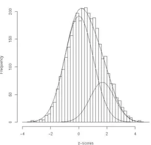
maximum) is given by πˆ = 0.65,0 µˆ1= 1.49, and σˆ12= 0.94. In Figure 1, we
dis-play the fitted mixture density superimposed on the histogram of zj-scores, along
with its two components, the theoretical N(0, 1) null density and the
N(1.49, 0.94) non-null density weighted by their prior probabilities of ˆπ and 0
(1-ˆπ ). It can be seen that this two-component normal mixture model gives a 0
good fit to the empirical distribution of the zj-scores.
In Table 1, we have listed the FDR estimated from (6) for various levels of the
threshold c0 in (5). It can be seen, for example, that if c0 is set equal to 0.1, then the
estimated FDR is0.06and Nr = 143 genes would be declared to be differentially
expressed. It is not suggested that the FDR should be controlled to be around
0.05. It is just that in this example, its control at this approximate level yields a number (143) of differentially expressed genes that is not too unwieldy for a bi-ologist to handle in subsequent confirmatory experiments; the choice of c0 is
dis-cussed in Efron (2005b).
TABLE 1
Estimated FDRand other error for various levels of the thresohold c0 applied to the posterior probability of
nondifferential expression for the breast cancer data, where Nr is the number of selected genes (with theoretical null)
0 c Nr nFDR nF N D R nF N R nF P R 0.1 0.2 0.3 0.4 0.5 143 338 539 743 976 0.06 0.11 0.16 0.21 0.27 0.32 0.28 0.25 0.22 0.18 0.88 0.73 0.60 0.48 0.37 0.004 0.02 0.04 0.08 0.13
In the original paper, Hedenfalk et al. (2001) selected 176 genes based on a modified F-test, with a p-value cut off of 0.001. Comparing genes which were se-lected in our set of 143, we found 107 in common, including genes involved in
DNA repair and cell death, which are over-expressed in BRCA1-mutation-positive
tumours, such as MSH2 (DNA repair) and PDCD5 (induction of apoptosis). Storey and Tibshirani (2003) in their analysis of this data set, selected 160 genes by thresholding genes with q-values less than or equal to α = 0.05 (an arbitrary cut-off value), of which there are 113 in common with our set of 143. Overall, 101 genes were selected in common to all three studies, with 24 genes unique to our set. We searched publicly available databases for the biological functions of these genes, and found these included DNA repair, cell cycle control and cell death,
Figure 1 – Breast cancer data: plot of fitted two-component normal mixture model with theoretical N(0, 1) null and non-null components (weighted respectively by ˆπ and (1 - 0 ˆπ )) imposed on his-0
togram of z-scores.
Among other analyses of this data set, π0 was estimated to be 0.52 by Broët et
al. (2004), 0.64 by Gottardo et al. (2006), 0.61 by Ploner et al. (2006), and 0.47 by
Storey (2002). In the fully parametric Bayesian approach of Broët et al. (2004), the mean of the null component was fixed at zero, but the variance was allowed to be free during the estimation process for computational convenience. In Ploner et al. (2006), 56 genes with highly extreme expression values were first removed as in Storey and Tibshirani (2003).
Concerning the other type of allocation rates for the choice of c0 = 0.1 (5), the
estimates of the FNDR, FNR,and FPR are equal to 0.32, 0.88, and 0.004, respec-tively. The FNR of 0.88 means that there would be quite a few false negatives
among the genes declared to be null (not differentially expressed). Analogous to the miss rate of Taylor et al. (2003), we might wish to have an idea of how many false negatives there would be in, say, the next best 57 genes with estimated pos-terior probability of nondifferential expression greater than c0 = 0.1, which takes
one down to the 200th best ranked gene. We can obtain an estimate of this
quan-tity by finding the average of the ˆτ (z1 j ) values for these next 57 genes. In the case
of c0 = 0.1, it is 0.89, implying that among the 57 next best genes (all declared to
be null genes), approximately 51 are actually non-null.
We also considered the fitting of the two-componet normal mixture model (16) with the null component mean and variance, µ0 and σ02, now estimated in
from Figure 2, the fit from using the empirical null in place of the N(0, 1) theo-retical null is similar to the fit in Figure 1.
In other analyses of this data set, Newton et al. (2001), Tusher et al. (2001), and Gottardo et al. (2006) concluded that there were 375, 374, and 291 genes, respec-tively, differentially expressed when the FDR is controlled at the 10% level. It can be seen from Table 1 that our approach gives 338 genes if a thresold of 0.2 is im-posed on the posterior probability of nondifferential expression for which the implied FDR is 11% and the FNR is 73%. The corresponding values with the use
of the empirical null can be from Table 2 to be 13% and 77% for the FDR and FNR,respectively, with 212 genes declared to be differentially expressed.
Figure 2 – Breast cancer data: plot of fitted two-component normal mixture model with empirical null and non-null components (weighted respectively by ˆπ and (1 - 0 ˆπ )) imposed on histogram of 0
z-scores.
TABLE 2
Estimated FDRand other error rates for various levels of the thresohold c0 applied to the posterior probability of
nondifferential expression for the breast cancer data, where Nr is the number of selected genes (with empirical null)
0 c Nr nFDR nF N D R nF N R F P R n 0.1 0.2 0.3 0.4 0.5 62 212 343 504 644 0.07 0.13 0.17 0.23 0.28 0.23 0.20 0.18 0.15 0.13 0.93 0.77 0.64 0.51 0.41 0.00 0.01 0.02 0.05 0.07
The (main) reason for fewer genes being declared differentially expressed with the use of the empirical than with the theoretical null is that the estimate of π0 is
empirical null would not be selected in favour of the theoretical N(0, 1) null. The same decision was reached too after we adopted a resembling approach (McLach-lan, 1987) to carry out a formal test of a theoretical versus empirical null, using the likelihood ratio test statistic.
9. CLUSTER ANALYSIS APPROACH
Another approach to this problem would be make to more assumptions and model the expression level for each gene. Then we can use the model-based pro-cedure EMMIX-WIRE of Ng et al. (2006) to cluster the gene profiles. More
specifi-cally, we let
1 2
( T, T T)
j =
y y y (22)
denote the expression profile for the jth gene, where
1 ( ,..., ) i T i = yij yijm y
denotes the vector containing the mi expression levels of the jth gene in Class i (i = 1, 2). That is, yijk denotes the expression level of the jth gene in the kth
mi-croarray experiment in the ith Class (i = 1, 2; j = 1, ..., N; k = 1, ..., mi), and m = m1 + m2.
We model the distribution of the profile vector yj for the jth gene by a g-component mixture with each component specified by a linear mixed model.
Conditional on its membership of the hth component of the mixture, we assume that yj follows a linear mixed-effects model (LMM),
,
j = h + hj+ h + hj
y Xβ Ub Vc ε (23)
where βh =(βh1, βh2)T is the vector of fixed effects (h = 1, ..., g). In (23), bhj =
(bh1j , bh2j)T and ch (a m-dimensional vector ) represent the unobservable gene- and
cluster-specific random effects, respectively, conditional on membership of the
hth cluster. The random effects bh and ch , and the measurement error vectors 1
(εhT,...,εhmT T) are assumed to be mutually independent, where X , U , and V are known design matrices of the corresponding fixed or random effects. Here the design matrices X and U are taken to be equal to the m × matrix with the first 2
m1 rows equal to (1, 0) and the next m2 = m – m1 rows equal to (0, 1), and V is
equal to Im , where the latter denotes the m m× identity matrix. The presence of
the random effect ch for the expression levels of genes in the hth component
in-duces a correlation between the profiles of genes within the same cluster.
With the LMM, the distributions of bhj and ch are taken, respectively, to be
mul-tivariate normal N2(0, Bh) and Nm(0, θchIm), where Im is the m m× identity matrix.
The presence of the random effect term bhj is to allow for correlation between the
ex-pression levels of a gene in different classes are uncorrelated. In an ideal experi-ment, one would hope that there would be no correlations between the tissue samples, and we could dispense with this random effects term bhj in the model.
The measurement error vector εhj is also taken to be multivariate normal Nm(0, Am), where Ah = diag(Hφh) is a diagonal matrix constructed from the
vec-tor (Hφh), where here H = X and φh =(σ σh21, h22)T. That is, we allow the hth
component variance to be different among the two classes of microarray experi-ments.
The vector Ψ of unknown parameters can be obtained by maximum likelihood via the EM algorithm, proceeding conditionally on the cluster-specific random
ef-fects ci. The E- and M-steps can be implemented in closed form. In particular, an
approximation to the E-step by carrying out time-consuming Monte Carlo meth-ods is not required. A probabilistic or an outright clustering of the genes into g components can be obtained, based on the estimated posterior probabilities of component membership given the profile vectors and the estimated cluster-specific random effects ˆ (ch h=1,..., )g .
Before we cluster the gene profiles, we normalized the expression levels in each gene profile so that they have mean zero and standard deviation one. With this normalization of the gene profiles, we fit a g = 3 component mixture model, where we let βh1 and βh2 denote the fixed effects for the means of the two classes.
The clustering of the gene profiles is not invariant under this normalization, but in our experience, it has proved to be a reasonable way to proceed. With this normalization, the intent to find three clusters where (a) for one cluster, the esti-mate of the fixed effects for the two class means are approxiesti-mately zero, (β11 ≈
β12 ≈ 0), corresponding to the genes that are not differentially expressed; (b) for a
second cluster, βˆ21<βˆ22, corresponding to genes that (before normalization) are upregulated more in Class C1 than in Class C2; (c) for a third cluster, βˆ31<βˆ32,
corresponding to genes that are downregulated more in Class C1 than in Class C2.
On fitting EMMIX-WIRE to the normalized gene profiles, we obtained three
clusters in proportions ˆπ = 0.63, 1 ˆπ = 0.14, 2 ˆπ = 0.23 3 with 1 ˆ β = (0.06, - 0.05)T, 2 ˆ β = (0.56,- 0.49)T, and 3 ˆ β =(- 0.42, 0.37)T. If we take the
genes in the first cluster to be the null genes, then our estimate of the proportion of null genes is ˆπ = 0.63, which is in general agreement with that obtained above 0
using the z-scores.
In Table 3, we have listed the FDR estimated from (6) for various levels of the
threshold c0. On comparing this table with Tables 1 and 2, it can be seen that for
approximately the same FDR level, we declare more genes to be differentially
ex-pressed but with a lower FNR by working with the full data (the gene profiles)
rather than the profiles in reduced form as summarized by their z-scores. How-ever, the validity of this approach in modelling the full data obviously depends on much stronger distributional assumptions.
TABLE 3
Estimated FDRand other error rates for various levels of the thresohold c0 applied to the posterior probability of
nondifferential expression for the breast cancer data, where Nr is the number of selected genes: clustering approach
0 c Nr nFDR FN D R n F N R n F P R n 0.1 0.2 0.3 0.4 0.5 257 480 678 854 1048 0.06 0.10 0.14 0.18 0.23 0.32 0.27 0.24 0.20 0.17 0.79 0.63 0.51 0.41 0.32 0.01 0.02 0.05 0.08 0.12
10. RESULTS FOR A DIFFERENT VERSION OF THE HEDENFALK DATA
Efron (2004) writes that “there is ample reason to distrust the theoretical null” in the case of the Hedenfalk data, whereas above we have found that the theo-retical and empirical null distributions are similar to each other. The difference in our findings may be due to the fact that our gene expression data seems to differ when compared with the expression data presented in Efron and Tibshirani (2002). Thus, the breast cancer data of Hedenfalk et al. (2001) that we have ana-lysed above is not the same as anaana-lysed in the papers of Efron (2004, 2005a, 2005b).
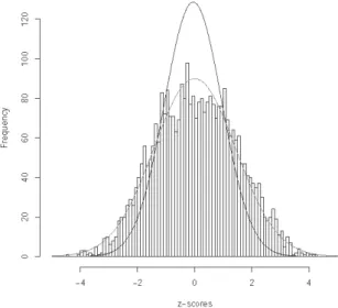
In Figure 3, we display the histogram of the z-scores as obtained by Efron (2004) for this data set, along with the N(0, 1) distribution and the N(0.05, 2.05) distribution with mean and variance equal to the sample mean and variance of the
z-scores. His z-score is defined to be
zj = Ф-1(F13(tj )), (24)
where tjis the pooled two-sample t-statistic and F13 is its distribution, which is the
t-distribution with 13 degrees of freedom. Thus non-null genes can have either
large positive or large negative values for z-scores. If we use the “empirical” dis-tribution N(0.05, 2.05) as the null disdis-tribution on its own (without a non-null component) then it can be seen from Figure 3 that no genes would be declared to be differentially expressed.
We now consider the two-component mixture normal approach applied to the same data as analysed in the papers of Efron. We did this by converting his sided z-scores to our one-sided ones. But before we considered fitting a two-component normal mixture to the latter, we need to address the question of whether we really need a non-null component in our model; that is, whether there are any genes that are differentially expressed (π0 = 1). We therefore carried out a
test of a single normal distribution with unspecified mean and variance (empirical null) versus a mixture of an empirical null and a non-null component. It was found in accordance with the conclusions of Efron that a single normal distribu-tion suffices.
Figure 3 – Breast cancer data: plot of N(0, 1) distribution and N(0.05, 2.05) imposed on the histo-gram of z-scores as analyzed in Efron’s papers.
11. DISTRIBUTION
In this paper, we consider the problem of detecting which genes are differen-tially expressed in multiple classes of tissue samples, where the classes represent various clinical or experimental conditions. The available data consist of the ex-pression levels of typically a very large number of genes for a limited number of tissues in each class. Usually, a test statistic such as the classical t in the case of two classes or the F in case of multiple classes is formed for a test of equality of the class means. The key step in this approach is to transform the observed value of the test statistic for each gene j to a z-score zjby using the inverse standard
normal distribution function of the implied P-value Pj, similar to its use in Efron
(2004) and his subsequent papers on this problem. Typically, a two-component normal mixture model is adequate for modelling the empirical distribution of the
zj-scores, where the first component is the standard normal, corresponding to the
null distribution of the score, and the second component is a normal density with unspecified (positive) mean and variance, corresponding to the non-null distribu-tion of the score. This model can be used to provide a staightforward and easily implemented assessment of whether a gene is null (not differentially expressed) in terms of its posterior probability of being a null gene. Estimates of this posterior probability can be easily obtained by using the EM algorithm to fit the
two-component normal mixture model via maximum likelihood. As there are multiple local maximizers, consideration has to be given to the choice of starting values for the algorithm. We show that the specification of an initial value ( 0 )
0
π for the
the normal mixture model with the teoretical choice of N(0, 1) as the null com-ponent. An interval of values for ( 0)
0
π can be tried, and a guide to its endpoints is given by values of π0 obtained by equating the number of zj values less than a
threshold ξ to the expected number under the theoretical N(0, 1) null component. We consider too the case where the theoretical N(0, 1) null is not tenable and an empirical null is adopted with the mean and the variance estimated from the data. Also, the estimation of the false discovery rate and its control are consid-ered, along with the estimation of other relevant rates such as the false negative rate. Note that it is not valid to make claims as to the relative superiority of the two models corresponding to the theoretical and empirical nulls on the basis of these error rates, as they are only valid for the model under which they were cal-culated.
Concerning the choice between the use of the theoretical N(0, 1) null and an empirical null, the intent in the first instance is to use the former in modelling the density of the zj-scores. In some situations, it will be clear that the use of the
theoretical null is inappropriate. In other situations, an informed choice between the theoretical and empirical null components can be made on the basis of the increase in the log likelihood due to the use of an empirical null with its two extra parameters. For this purpose we can use BIC or a resampling approach to assess
the P-value of a formal test based on the likelihood ratio test statistic. Recent re-sults of the authors suggest that the latter approach is preferable to the use of BIC
in this context.
In the version of the Hedenfalk data as analysed the papers by Efron, it ap-pears that there are no genes that are differentially expressed. Hence in general before we proceed to fit a two-component normal mixture model with either a theoretical or an empirical null, the question of whether a single normal distribu-tion is adequate needs to be considered first in situadistribu-tions where it is not obvious that there are some genes present that are differentially expressed.
The reliability of our approach obviously depends on how well the proposed two-component normal mixture model approximates the empirical distribution of the zj-scores. Its fit can be assessed either by visual inspection of a plot of the
fitted normal mixture density versus a histogram of the zj-scores or, more
for-mally, by a likelihood ratio test for the need for an additional normal density to represent the non-null distribution of the zj-scores. On a similar note on the
ade-quacy of a two-component normal mixture model, Pounds and Morris (2003) found that a two-component mixture of the uniform (0, 1) distribution and a sin-gle beta component (with one unspecified unknown parameter) was adequate to model the distribution of the P-values in their analyses. However, it is advanta-geous to work as proposed here in terms of the zj-scores, which can be modelled
by normal components on the real line rather than working in terms of the
P-values.
Finally, we should mention explicitly that the adoption of the standard normal for the null distribution is equivalent to assuming that the genes are all independ-ently distributed. Typically in practice, this independence assumption will not
hold for all the genes. As cautioned by Qiu et al. (2005), care is needed in extrapo-lating results valid in the case of independence to dependent gene data.
Department of Mathematics GEOFF. J. MCLACHLAN
University of Queensland,Australia
and ARC Centre of Excellence in Bioinformatics, Institute for
Molecular Bioscience, University of Queensland,Australia
Department of Mathematics KENT WANG
University of Queensland,Australia SHU KAY NG
REFERENCES
D.B. ALLISON, G.L. GADBURY, M. HEO, J.R. FERNANDEZ, C.-K. LEE, T.A. PROLLAandR. WEINDRUCH
(2002), A mixture model approach for the analysis of microarray gene expression data., “Computa-tional Statistics & Data Analysis”, 39, pp. 1-20.
Y. BENJAMINIandY. HOCHBERG(1995), Controlling the false discovery rate: a practical and powerful
approach to multiple testing, “Journal of the Royal Statistical Society”, B57, pp. 289-300.
P. BROËT, A. LEWIN, S. RICHARDSON, C. DALMASSOandH. MAGDELENAT(2004), A mixture model-
based strategy for selecting sets of genes in multiclass response microarray experiments,
“Bioinformat-ics”, 20, pp. 2562-2571.
A.P. DEMPSTER, N.M. LAIRDandD.B. RUBIN(1977), Maximum likelihood from incomplete data via the
EM algorithm (with discussion). “Journal of the Royal Statistical Society”, B39, pp. 1-38.
K.-A. DO, P. MÜLLERandF. TANG(2005), A Bayesian mixture model for differential gene expression. “Applied Statistics”, 54, 627-644.
B. EFRON(2004),Large-scale simultaneous hypothesis testing: the choice of a null hypothesis, “Journal of the American Statistical Association”, 99, 96-104.
B. EFRON(2005a),Selection and Estimation for Large-Scale Simultaneous Inference, “Technical Re-port”, Stanford, CA: Department of Statistics, Stanford University, http://www-stat.stanford.edu/˜brad/papers/Selection.pdf.
B. EFRON(2005b),Local False Discovery Rates. “Technical Report”, Stanford, CA: Depart-ment of Statistics, Stanford University, http://www-stat.stanford.edu/˜brad/papers/ False.pdf.
B. EFRON, R. TIBSHIRANI(2002), Empirical Bayes methods and false discovery rates for microarrays,
“Genetic Epidemiology.”, 23, pp. 70-86.
B. EFRON, R. TIBSHIRANI, J.D. STOREYandV.G. TUSHER(2001),Empirical Bayes analysis of a
microar-ray experiment, “Journal of the American Statistical Association”, 96, pp. 1151-1160.
R. GOTTARDO, A.E. RAFTERY, K.Y. YEUNGandR.E. BUMGARNER(2006), Bayesian robust inference for
differential gene expression in cDNA microarrays with multiple samples, “Biometrics”, 62, to appear.
X. GUO, W. PAN(2005), Using weighted permutation scorse to detect differential gene expression with
mi-croarray data, “Journal of Bioinformatics and Computational Biology”, 3, pp. 989-1006.
I. HEDENFALK et al. (2001), Gene-expression profiles in hereditary breast cancer, “The New England Journal of Medicine”, 344, pp. 539-548.
M.-L.T. LEE, F.C. KUO, G.A. WHITMOREandJ. SKLAR(2000), Importance of replication in microarray
gene expression studies: statistical methods and evidence from repetitive cDNA hybridizations,
“Pro-ceedings of the National Academy of Science”, USA 97,pp. 9834-9838.
I. LÖNNSTEDT, T. SPEED(2002)Replicated microarray data, “Statistica Sinica”, 12, pp. 31-46.
G.J. MCLACHLAN(1987), On bootstrapping the likelihood ratio test statistic for the number of
G.J. MCLACHLAN, R.W. BEANandL. BEN-TOVIM JONES(2006), A simple implementation of a normal
mixture approach to differential gene expression in multiclass microarrays, “Bioinformatics”, 22,
pp. 1608-1615.
G.J. MCLACHLAN, K.-A. DOandC. AMBROISE(2004), Analyzing Microarray Gene Expression Data, Wiley, Hoboken, New Jersey.
G.J. MCLACHLAN, T. KRISHNAN(1997), The EM Algorithm and Extensions, Wiley, New York.
G.J. MCLACHLAN, D. PEEL(2000), Finite Mixture Models, Wiley, New York.
M.A. NEWTON, C.M. KENDZIORSKI, C.S. RICHMOND, F.R. BLATTNERand K.W. TSUI(2001), On
differen-tial variability of expression ratios: improving statistical inference about gene expression changes from
microarray data, “Journal of Computational Biology”, 8, pp. 37-52.
M.A. NEWTON, A. NOUEIRY, D. SARKARandP. AHLQUIST(2004), Detecting differential gene expression
with a semiparametric hierarchical mixture method, “Bioinformatics”, 5, pp. 155-176.
W. PAN(2002), A comparative review of statistical methods for discovering differentially expressed genes
in replicated microarray experiments, “Bioinformatics”, 18, pp. 546-554.
W. PAN(2003), On the use of permutation in and the performance of a class of nonparametric methods to
detect differential gene expression,“Bioinformatics”, 19, pp. 1333-1340.
W. PAN, J. LINandC.T. LE(2003), A mixture model approach to detecting differentially expressed genes
with microarray data. Model-based cluster analysis of microarray gene-expression data, “Genome
Biology”, 3, research0009.1-0009.8.
Y. PAWITAN, S. MICHIELS, S. KOSCIELNY, A. GUSNANTOandA. PLONER(2005), False discovery rate,
sensitivity and sample size for microarray studies, “Bioinformatics”, 21, pp. 3017-3024.
A. PLONER, S. CALZA, A. GUSNANTOandY. PAWITAN(2006), Multidimensional local false discovery rate
for microarray studies, “Bioinformatics”, 22, pp. 556-565.
S. POUNDS, S.W. MORRIS(2003), Estimating the occurrence of false positives and false negatives in
mi-croarray studies by approximating and partitioning the empirical distribution of p-values,
“Informat-ics”, 19, pp. 1236-1242.
X. QIU, L. KLEBANOVandA. YAKOVLEV(2003), Correlation between gene expression levels and
limita-tions of the empirical Bayes methodology for finding differentially expressed genes, “Statistical
Appli-cations in Genetics and Molecular Biology”, 4, n. 1, Article 34.
G.K. SMYTHY(2004), Linear models and empirical Bayes methods for assessing differential expression in
microarray experiments, “Statistical Applications in Genetics and Molecular Biology”, 3, n.
1, Article 3.
J.D. STOREY(2002), A direct approach to false discovery rates, “Journal of the Royal Statistical So-ciety”, B 64, pp. 479-498.
J.D. STOREY, R. TIBSHIRANI(2003), Statistical significance for genome-wide studies, “Proceedings of the National Academy of Sciences”, USA 100, pp. 9440-9445.
J. TAYLOR, R. TIBSHIRANIandB. EFRON(2005), The ‘miss rate’ for the analysis of gene expression data, “Biostatistitics”, 6, pp. 111-117.
V.G. TUSHER, R. TIBSHIRANIandG. CHU(2001), Significance analysis of microarrays applied to the
ion-izing radiation response, “Proceedings of the National Academy of Sciences”, USA 98, pp.
5116-5121.
A.B. VAN’T WOUTet al. (2003), Cellular gene expression upon human immunodeficiency virus type 1
infection of CD4+-T-cell linear, “Journal of Virology”, 77, pp. 1392-1402.
E.B. WILSONandM.M. HILFERTY(1931), The distribution of chi-square, “Proceedings of the Na-tional Academy of Sciences”, USA28, pp. 94-100.
Y. XIE, W. PANandA.B. KHODURSKY(2005), A note on using permutation-based false discovery rate
estimate to compare different analysis methods for microarray data, “Bioinformatics”, 21, pp.
4280-4288.
Y. ZHAO, W. PAN(2003), Modified nonparametric approaches to detecting differentially expressed genes in
SUMMARY
Large-scale simultaneous inference with applications to the detection of differential expression with microarray data
An important problem in microarray experiments is the detection of genes that are dif-ferentially expressed in agiven mumber of classes. We consider a straightforward and eas-ily implemented method for estimating the posterior probability that an individual gene is null. The problem can be expressed in a two-component mixture framework, using an empirical Bayes approach. Current methods of implementing this approach either have some limitations due to the minimal assumptions made or with more specific assump-tions are computationally intensive. By converting to a z-score the value of the test statis-tic used to test the significance of each gene, we can use a simple two-component normal mixture to model adequately the distribution of this score. In the context of the applica-tion of this approach to a well known breast cancer data set, we consider some of the is-sues associated with the problem of the detection of differential expression, including the case where there is need for the use of an empirical null distribution in place of the stan-dard normal (the theoretical null) and the case where none of the genes might be differen-tially expressed. We also describe briefly some initial results on a cluster analysis approach to this problem, which attempts to model the joint distribution of the individual gene ex-pressions. This latter approach thus has to make distributional assumptions which are note necessary with the former approach based on the z-scores. However, in the case where the distributional assumptions are valid, it has the potential to provide a more powerful analysis.