View of Use of Double Sampling Scheme in Estimating the Mean of Stratified Population under Non-response

(1)

USE OF DOUBLE SAMPLING SCHEME IN ESTIMATING THE

MEAN OF STRATIFIED POPULATION UNDER

NON-RESPONSE

Manoj K. Chaudhary1

Department of Statistics, Banaras Hindu University, Varanasi, India

Amit Kumar

Department of Statistics, Banaras Hindu University, Varanasi, India

1. Introduction

Auxiliary information can be used to improve the efficiency of the estimator of a particular population parameter. The effectiveness of the estimation procedure with the use of auxiliary information closely depends upon the method in which the estimator has been proposed, i.e., the form in which the functions of auxiliary information have been considered. There is a lot of works in which the auxil-iary information are used to enhance the precision of the estimator. Upadhyaya and Singh (1999) have suggested a class of estimators for estimating the popu-lation mean in simple random sampling. Kadilar and Cingi (2003) and Shabbir and Gupta (2005) expanded these estimators for estimating the population mean of stratified population. Singh et al. (2012) have proposed a general family of estimators for estimating the population mean in systematic sampling.

We know that the problem of non-response is inherent in the population of every survey. The non-response error is not so important if the characteristics of the non-responding units are similar to those of the responding units. But, it is noticed that such similarity of characteristics between two types of units (responding and non-responding units) is not always obtained in practice. Hansen and Hurwitz (1946) introduced a technique of sub-sampling of non-respondents in order to adjust the non-response in mail surveys. Khoshnevisan et al. (2007) have proposed a general family of estimators of population mean using known coeﬃcients of some population parameters in simple random sampling. Chaudhary

et al. (2009) have proposed a combined-type family of estimators with the use of

an auxiliary variable for mean of a stratiﬁed population in the presence of non-response adopting Khoshnevisan et al. (2007). Recently, Chaudhary and Singh (2013) have proposed factor type families of estimators of population mean in two-stage sampling with equal size clusters under non-response.

(2)

It is well known fact that when the parametric values of auxiliary variable are not known, one can utilize the double sampling (or two-phase sampling scheme) in improving the estimation procedure. Two-phase sampling is very eﬀective in terms of cost as well as applications. This sampling scheme is used to obtain the information about auxiliary variable inexpensively from a larger sample at ﬁrst phase and comparatively small sample at the second phase. Okafor and Lee (2000) have discussed the method of double sampling scheme for estimating the family expenditure in a household survey under non-response. Khare and Sinha (2004) have suggested the estimators for population ratio using two-phase sampling scheme in the presence of non-response.

In the light of above context, we have suggested a family of combined-type es-timators of population mean in stratiﬁed random sampling using two-phase sam-pling scheme under non-response whenever the population mean of auxiliary vari-able is unknown. The properties of the family along with its optimum property have been discussed.

2. Notations, Sampling Strategy and Estimation Procedure

yij: Observation on the jthunit in the ithstratum under study variable.

(i = 1, 2, ..., k; j = 1, 2, ..., Ni) .

xij : Observation on the jthunit in the ithstratum under auxiliary variable.

(i = 1, 2, ..., k; j = 1, 2, ..., Ni) .

Ni1: Population size of the response group in the ithstratum.

Ni2: Population size of non-response group in the ithstratum.

Y =∑k_i=1piYi: Population mean under study variable.

X =∑k_i=1piXi: Population mean under auxiliary variable.

Yi= _N1_i

∑Ni

j=1yij: Population mean of the ithstratum under study variable.

Xi=_N1

i ∑Ni

j=1xij: Population mean of the i

th_{stratum under auxiliary variable.}

Yi2 = _N1_i2

∑Ni2

j yij: Population mean of the non-response group in the ith

stra-tum under study variable.

xi=_n1

i ∑ni

j xij: Sample mean of the i

th_{stratum under auxiliary variable.}

x′_i= 1

n′_i

∑n′_i

j xij: Mean based on ﬁrst phase sample in the ithstratum under

(3)

y_ni1= _n1 i1

∑ni1

j yij: Sample mean of the response group in the ithstratum under

study variable.

y_hi2 = _h1 i2

∑hi2

j yij: Mean based on hi2 non-respondent units in the i

th _stratum

under study variable.

S2 Y i = 1 Ni−1 ∑Ni j=1 ( yij− Yi )2

: Population mean square of the ith_{stratum under}

study variable. S_Xi2 = _N1 i−1 ∑Ni j=1 ( xij− Xi )2

: Population mean square of the ithstratum under auxiliary variable. S2 Y i2 = 1 Ni2−1 ∑Ni2 j ( yij− Yi2 )2

: Population mean square of the non- response group in the ith_{stratum under study variable.}

Wi1= N_Ni1

i: Response rate in the i

th_stratum.

Wi2= N_Ni2

i: Non-response rate in the i

th_stratum.

Let us suppose that a population of size N is divided into k strata. Let the size of the ith stratum be Ni (i = 1, 2, ..., k) such that

∑k

i=1Ni = N . Let a sample of

size n be selected from the entire population in such a way that niunits are selected

from the ith stratum and we have∑k_i=1ni = n. Let Y be the study variable with

population meanY = ∑k_i=1piYi(Yi being the mean of the ithstratum based on

Ni units and pi =N_Ni) and we assume that the non-response is observed on study

variable. It is observed that there are ni1respondent units and ni2non-respondent

units in ni units. Using Hansen and Hurwitz (1946) technique of sub-sampling

of non-respondents, we select a sub-sample of hi2 units out of ni2 non-respondent

units such thatni2 = Lihi2, Li ≥ 1and collect the information from all hi2 units.

Thus, an unbiased estimator of population mean Y is given by

y∗_st=

k

∑

i=1

piy∗i (1)

where y∗_i = ni1yni1+ni2yhi2

ni ,

y_ni1 and y_hi2 are the means based on ni1 respondent units and hi2sub-sampled

non-respondent units respectively. The variance of y∗_st is given as

V (y∗st) = k ∑ i=1 ( 1 ni − 1 Ni ) p2iSY i2 + k ∑ i=1 (Li− 1) ni Wi2p2iSY i22 (2) where S2 Y iand S 2

Y i2are the population mean squares of the entire group and

non-response group respectively in ith_{stratum for study variable. W}

i2is the population

non-response rate in the ith_stratum.

In order to improve the eﬃciency of an estimator, one can utilize the auxiliary information at the estimation stage. In this sequence, Chaudhary et al. (2009)

(4)

have proposed a family of combined-type estimators of population mean using an auxiliary variable X in stratiﬁed random sampling under the condition that the non-response is observed on study variable and auxiliary variable is free from non-response, given as TC = y∗st [ aX + b α (ax_st+ b) + (1− α)(aX + b) ]g (3) where x_st=∑k_i=1pixi, X = ∑k

i=1piXi (population mean of auxiliary variable),

a̸= 0 and bare either real numbers or functions of known parameters of auxiliary

variable. α and gare the constants and to be determined. xi and Xi are

respec-tively the mean based on ni units and mean based on Ni units in the ithstratum

for auxiliary variable. The bias and mean square error (MSE) of TC up to the

ﬁrst order of approximation are respectively given by

B (TC) = 1 ¯ Y k ∑ i=1 fip2i [ g(g + 1) 2 α 2_λ2_R2_S2 Xi− αλgRρiSXiSY i ] (4) and M SE (TC) = k ∑ i=1 fip2i [ S_{Y i}2 + α2λ2g2R2S_Xi2 − 2αλgRρiSXiSY i ] + k ∑ i=1 (Li− 1) ni Wi2p2iSY i22 (5) where fi= ( 1 ni− 1 Ni ) , λ = aX aX+b, R = Y X, S 2

Xi is the population mean square of

auxiliary variable for the ith_{stratum and ρ}

iis the population correlation coeﬃcient

between Y and X in the ith_stratum.

3. Proposed Family of Estimators

If the population mean of auxiliary variable X is known, one can easily use the family of estimators shown in equation (3) for estimating the population mean of study variableY . But if the population mean X is unknown, it is not easy to adopt the present form of the considered family of estimators. Thus the double sampling scheme (or two-phase sampling scheme) can be utilized to estimate the population meanY . Adopting double sampling scheme ﬁrst the estimate of Xmay be generated from a large ﬁrst phase sample of size n′_i drawn from the Ni units

by simple random sampling without replacement (SRSWOR) scheme for the ith

stratum. Secondly, a smaller second phase sample of size niis drawn from n

′

iunits

by SRSWOR. It is noted that the non-response is observed on study variable at second phase sample. Out ofni units, let ni1units respond and ni2 units do not

respond at the second phase. Applying Hansen and Hurwitz (1946) technique of sub-sampling of non-respondents, a sub-sample of hi2(= ni2/Li, Li≥ 1) units is

(5)

selected from the sample of ni2 non-respondents and the information is collected

from all of them.

Let us assume that the full information is supplied on the n′_i units at the ﬁrst phase for the auxiliary variable Xand the study variable goes through the non-response. Thus the usual combined ratio and product estimators of population mean Y using two-phase sampling scheme in stratiﬁed random sampling under non-response are respectively given by

T1∗= y∗st xst x′st (6) and T₂∗= y ∗ st x′_stxst (7) where x′_st=∑k_i=1pix ′ i and x ′

iis the mean based on n

′

i units for auxiliary variable.

The mean square errors (MSEs) of the estimators T₁∗ and T₂∗ up to the ﬁrst order of approximation are respectively given by

M SE (T1∗) = k ∑ i=1 fi′p 2 iS 2 Y i+ k ∑ i=1 fi∗p 2 i ( SY i2 + R 2 SXi2 − 2RρiSXiSY i ) + k ∑ i=1 (Li− 1) ni Wi2p2iS 2 Y i2 (8) and M SE (T₂∗) = k ∑ i=1 f_i′p2_iS2_{Y i}+ k ∑ i=1 f_i∗p2_i(S_{Y i}2 + R2S_Xi2 + 2RρiSXiSY i ) + k ∑ i=1 (Li− 1) ni Wi2p2iS 2 Y i2 (9) where f_i′ = ( 1 n′_i − 1 Ni ) and f_i∗= ( 1 ni − 1 n′_i ) .

In the presence of above circumstances, a family of combined-type estimators of mean Y of stratiﬁed population using two-phase sampling in the presence of non-response is given by T_C′ = y∗_st [ ax′st+ b α (ax_st+ b) + (1− α)(ax′_st+ b) ]g (10)

In order to obtain the bias and MSE of T_C′, we use large sample approximation. Let us assume that

y∗_st= Y (1 + e0) , xst= X (1 + e1) , x ′ st= X ( 1 + e′₁ ) .

Form the above, we have

E (e0) = E (e1) = E

(

e′₁

) = 0,

(6)

E(e2₀)= 1 Y2 k ∑ i=1 [( 1 ni − 1 Ni ) p2_iS_{Y i}2 +(Li− 1) ni Wi2p2iS 2 Y i2 ] , E(e2₁)= 1 X2 k ∑ i=1 ( 1 ni − 1 Ni ) p2_iS_Xi2 , E ( e′₁2 ) = 1 X2 k ∑ i=1 ( 1 n′_i − 1 Ni ) p2_iS2_Xi, E (e0e1) = 1 XY k ∑ i=1 ( 1 ni − 1 Ni ) p2_iρiSY iSXi, E ( e0e ′ 1 ) = 1 XY k ∑ i=1 ( 1 n′_i − 1 Ni ) p2_iρiSY iSXi, E ( e1e ′ 1 ) = 1 X2 k ∑ i=1 ( 1 n′_i − 1 Ni ) p2_iS_Xi2 .

Putting the above assumptions into equation (10), T_C′ can be expressed as

T_C′ = Y (1 + e0) ( 1 + λe′₁ )g[ 1 + λ { αe1+ (1− α) e′₁ }]_−g (11) On expanding equation (11) and neglecting the terms ofe0, e1and e

′

1having

power greater than two, we get

T_C′ − Y = Y [ −gλ{αe1+ (1− α) e′₁ } +g (g + 1) 2 λ 2{_α2_e2 1+ (1− e) 2 e′₁2 +2α (1− α) e1e′₁ } + gλe′₁− g2λ2e′₁ { αe1+ (1− α) e ′ 1 } + g (g− 1) 2 λ 2_e′2 1 + e0− gλe0 { αe1+ (1− α) e′₁ } + gλe′₁e0 ] (12)

Taking expectation both the sides of equation (12), we get bias of T_C′ up to the ﬁrst order of approximation as

B ( T_C′ ) = 1 Ygλ k ∑ i=1 p2_i [ fi { (g + 1) 2 λα 2_R2_S2 Xi− 2RρiSY iSXi } + f_i′ {( (g + 1) 2 λ (1− α) 2 R2+ (g + 1) λα (1− α) R2− gλR2 +(g− 1) 2 λR 2 ) S2_Xi+ RαρiSY iSXi }] (13)

Squaring both the sides of the equation (12) and then taking the expectation by neglecting the terms ofe0, e1and e

′

1having power greater than two, we get MSE

of T_C′ up to the ﬁrst order of approximation as

M SE ( T_C′ ) = g2λ2R2α2 k ∑ i=1 f_i∗p2_iS2_Xi− 2gλRα k ∑ i f_i∗p2_iρiSXiSY i + k ∑ i=1 fip2iS 2 Y i+ k ∑ i=1 (Li− 1) ni Wi2p2iS 2 Y i2 (14)

(7)

or M SE ( T_C′ ) = k ∑ i=1 f_i′p2_iS_{Y i}2 + k ∑ i=1 f_i∗p2_i(S_{Y i}2 + g2λ2R2α2S_Xi2 −2gλRαρiSXiSY i) + k ∑ i=1 (Li− 1) ni Wi2p2iS2Y i2 (15) 3.1 Optimum Choice of α

In this section, we choose the optimum value of α for which the MSE of the proposed family would remain its minimum. On diﬀerentiating M SE

(

T_C′

) with respect to α and equating the derivative to zero, we get

∂M SE ( T_C′ ) ∂α = 2g 2_λ2_R2_α k ∑ i=1 f_i∗p2_iS_Xi2 − 2gλR k ∑ i f_i∗p2_iρiSXiSY i= 0 (16) ⇒ αopt= ∑k i fi∗p 2 iρiSXiSY i gλR∑k_i=1f_i∗p2 iSXi2 (17) On substituting the value of αopt from equation (17) into equation (14) or

equation (15), we get the minimum MSE of T_C′. 3.2 Cost of the Survey and Optimumni,n

′ i, Li

Let c′_i be the cost per unit associated with the ﬁrst phase sample of size n′_i and

ci0 be the unit cost of ﬁrst attempt on study variable with second phase

sam-ple of sizeni. Let ci1and ci2 be respectively the cost per unit of enumerating the

ni1respondent units and hi2 non-respondent units. Then the total cost for the ith

stratum is given by Ci= c ′ in ′ i+ ci0ni+ ci1ni1+ ci2hi2 ∀i = 1, 2, ..., k.

Now, we obtain the expected cost per stratum as

E (Ci) = c ′ in ′ i+ ni ( ci0+ ci1Wi1+ ci2 Wi2 Li ) .

Thus the total cost over all the strata is represented as

C0= k ∑ i=1 E (Ci) = k ∑ i=1 [ c′_in′_i+ ni ( ci0+ ci1Wi1+ ci2 Wi2 Li )] . (18)

(8)

Let us consider the Lagrange function ϕ = M SE ( T_C′ ) + µC0 (19)

where µ is Lagrange’s multiplier.

In order to get the optimum values ofni, n

′

iandLi, we diﬀerentiate ϕ with respect toni, n

′

iand Li respectively and equate the derivatives to zero. Thus, we have ∂ϕ ∂ni =−p 2 i n2 i ( SY i2 + g 2 λ2R2α2SXi2 − 2gλRαρiSXiSY i ) −(Li− 1) n2 i Wi2p2iS 2 Y i2 +µ ( ci0+ ci1Wi1+ ci2 Wi2 Li ) = 0 (20) ∂ϕ ∂n′_i = p2 i n′2 i ( g2λ2R2α2S_Xi2 − 2gλRαρiSXiSY i ) + µc′_i= 0 (21) ∂ϕ ∂Li =p 2 i ni Wi2SY i22 − µnici2 Wi2 L2 i = 0 (22)

From equations (20), (21) and (22), we respectively get

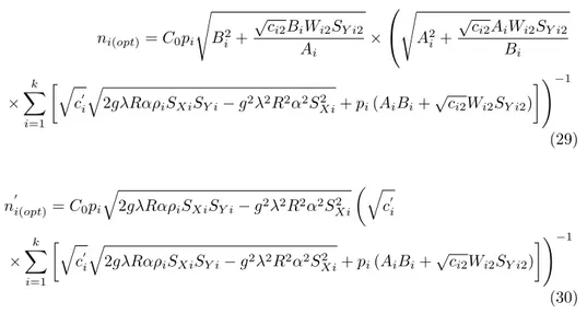
ni= pi √ S2 Y i+ g2λ2R2α2S 2 Xi− 2gλRαρiSXiSY i+ (Li− 1) Wi2SY i22 √ µ ( ci0+ ci1Wi1+ ci2WLi2i ) (23) n′_i= pi √ 2gλRαρiSXi_√SY i− g2λ2R2α2SXi2 µc′_i (24) and √_{µ =}piLiSY i2 ni√ci2 (25) Putting the value of√µ from equation (25) into equation (23), we get

Li(opt)= √ ci2Bi SY i2Ai (26) where Ai= √ ci0+ ci1Wi1 and Bi= √ S2 Y i+ g2λ2R2α2SXi2 − 2gλRαρiSXiSY i− Wi2S2Y i2.

On substituting the value of Li(opt) from equation (26) into equation (23), we

can express ni as ni= pi √ B2 i + √_c i2BiWi2SY i2 Ai √_µ√_A2 i + √_c i2AiWi2SY i2 Bi (27)

In obtaining the value of√µ in terms of total costC0, we put the values of n

′

i,

Li(opt) and ni from equations (24), (26) and (27) into equation (18). Thus, we

(9)

TABLE 1 Particulars of Data Stratum No. Ni n ′ i ni Yi Xi SY i2 S2Xi ρi SY i22 1 73 65 26 40.85 39.56 6369.10 6624.44 0.999 618.88 2 70 25 10 27.83 27.57 1051.07 1147.01 0.998 240.91 3 97 48 19 25.79 25.44 2014.97 2205.40 0.999 265.52 4 44 11 5 20.64 20.36 538.47 485.27 0.997 83.69 √ µ = 1 C0 k ∑ i=1 [√ c′_i √ 2gλRαρiSXiSY i− g2λ2R2α2SXi2 + pi(AiBi+√ci2Wi2SY i2) ] (28) Substituting the value of√µ from equation (28) into equations (27) and (24),

we respectively get the optimum values of ni and n

′ i ni(opt)= C0pi √ B2 i + √_c i2BiWi2SY i2 Ai ×   √ A2 i + √_c i2AiWi2SY i2 Bi × k ∑ i=1 [√ c′_i √ 2gλRαρiSXiSY i− g2λ2R2α2SXi2 + pi(AiBi+ √ ci2Wi2SY i2) ])−1 (29) n′_i(opt)= C0pi √ 2gλRαρiSXiSY i− g2λ2R2α2SXi2 (√ c′_i × k ∑ i=1 [√ c′_i √ 2gλRαρiSXiSY i− g2λ2R2α2S_Xi2 + pi(AiBi+√ci2Wi2SY i2) ])−1 (30) 4. Empirical Study

The theoretical study of the proposed family can easily be comprehended by an empirical analysis. To support the theoretical results, we have used the data considered by Chaudhary et al. (2012). There are 284 municipalities divided into four strata having respective sizes 73, 70, 97, and 44. The data relate to the population size (in thousands) in the year 1985 as study variable and the population size (in thousands) in the year 1975 as auxiliary variable. Particulars are given in Table 1.

Table 2 represents the MSE and percent relative eﬃciency (PRE) of T₁∗, T₂∗ and T_C′ (at α(opt), a = 1, b = 1 and g = 1)with respect to y∗st for the diﬀerent

(10)

414 M. K. Chaudhary and A. TABLE 2 MSE and PRE of T1∗, T2∗ and T

′ C with respect to y∗st Wi2 Li V (y∗st) M SE (T1∗) M SE (T2∗) M SE ( T_C′ ) P RE (T₁∗) P RE (T₂∗) P RE ( T_C′ ) 2 34.42 23.62 375.17 6.28 145.72 9.17 548.09 0.1 2.5 34.67 24.01 375.56 6.54 144.40 9.23 530.12 3 34.92 24.41 375.96 6.79 143.06 9.29 514.29 3.5 35.18 24.8 376.35 7.04 141.85 9.35 499.72 2 34.92 24.41 375.96 6.79 143.06 9.29 514.29 0.2 2.5 35.43 25.2 376.75 7.3 140.60 9.40 485.34 3 35.94 25.99 377.54 7.8 138.28 9.52 460.77 3.5 36.44 26.78 378.33 8.31 136.07 9.63 438.51 2 35.43 25.2 376.75 7.3 140.60 9.40 485.34 0.3 2.5 36.19 26.38 377.93 8.06 137.19 9.58 449.01 3 36.95 27.57 379.12 8.82 134.02 9.75 418.93 3.5 37.71 28.75 380.3 9.57 131.17 9.92 394.04 2 35.94 25.99 377.54 7.8 138.28 9.52 460.77 0.4 2.5 36.95 27.57 379.12 8.82 134.02 9.75 418.93 3 37.96 29.14 380.69 9.83 130.27 9.97 386.16 3.5 38.97 30.72 382.27 10.84 126.86 10.19 359.50

(11)

From the Table 2, it is revealed that the optimum estimator of the proposed family certainly provides the better estimates as compared to y∗_st, T₁∗ andT₂∗. It is obvious that the increment in population non-response rate Wi2 or inverse

sampling rate Li would cause a further increment in the MSE of the estimators.

Thus, from the above table (Table 2), it is also revealed that the eﬃciency of the estimators decreases with an increase in non-response rate Wi2 as well as with an

increase in inverse sampling rate Li.

5. CONCLUSION

The use of auxiliary information certainly improves the precision of the estimator at the estimation stage. The situations in which the parametric values of auxil-iary variable(s) are not known, one can use its estimates by using double sampling scheme in estimating the parameters of study variable. To cope up the situa-tions, we have proposed a family of combined-type estimators of population mean in stratified random sampling using double sampling scheme under non-response. The optimum combined-type estimator of the family has been obtained and com-parison of it with the usual mean, usual combined ratio and usual combined prod-uct estimators has also been made. The optimum values of first phase sample sizen′_i, second phase sample size ni and inverse sampling rate Li for the different

strata through the proposed family, have been determined under the cost survey. From Table 2, it is observed that the optimum combined-type estimator of the proposed family provides better estimates than the usual mean, usual combined ratio and usual combined product estimators. It is also observed that precision of the optimum combined-type estimator as well as usual mean, usual combined ratio and usual product estimators decreases with increase in non-response rate and inverse sampling rate. The results are intuitively expected.

Acknowledgements

The authors are thankful to the learned referees for their constructive suggestions regarding improvement of the present paper.

References

M. K. Chaudhary, R. Singh, R. K. Shukla, M. Kumar (2009). A family

of estimators for estimating population mean in stratified sampling under non-response. Pakistan Journal of Statistics and Operation Research, 5, no. 1, pp.

47–54.

M. K. Chaudhary, V. K. Singh (2013). Estimating the population mean in

two- stage sampling with equal size clusters under non-response using auxiliary characteristic. Mathematical Journal of Interdisciplinary Sciences, 2, no. 1, pp.

43–55.

M. K. Chaudhary, V. K. Singh, R. K. Shukla (2012). Combined-type

(12)

non-response. Journal of Reliability and Statistical Studies (JRSS), 5, no. 2, pp.

133–142.

M. H. Hansen, W. N. Hurwitz (1946). The problem of non-response in sample

surveys. Journal of The American Statistical Association, , no. 41, pp. 517–529.

C. Kadilar, H. Cingi (2003). Ratio estimators in stratified random sampling. Biometrical journal, 2, no. 45, pp. 218–225.

B. B. Khare, R. R. Sinha (2004). Estimation of finite population ratio using

two-phase sampling scheme in the presence of non-response. Aligarh J. Stat.,

24, 43-56., 24, pp. 43–56.

M. Khoshnevisan, R. Singh, P. Chauhan, N. Sawanand, F. Smarandache (2007). A general family of estimators for estimating population mean using

known value of some population parameter(s). Far East Journal of Theoretical

Statistics, 22, pp. 181–191.

F. C. Okafor, H. Lee (2000). Double sampling for ratio and regression

esti-mation with sub-sampling the non-respondents. Survey Methodology, 26, pp.

183–188.

J. Shabbir, S. Gupta (2005). Improved ratio estimators in stratified sampling. American Journal of Mathematical and Management Sciences, 25, no. 3-4, pp. 293–311.

R. Singh, S. Malik, M. K. Chaudhary, H. K. Verma, A. A. Adewara (2012). A general family of ratio-type estimators in systematic sampling. Journal of Reliability and Statistical Studies, 5, no. 1, pp. 73–82.

L. N. Upadhyaya, H. P. Singh (1999). Use of transformed auxiliary variable

in estimating the finite population mean. Biometrical Journal, 41, no. 5, pp.

627–636.

Summary

The present paper focuses on the use of double sampling scheme in stratified random sampling for estimating the population mean in the presence of non-response. Motivated by Khoshnevisan et al. (2007), we have proposed a family of combined-type estimators of population mean utilizing the information on an auxiliary variable with the use of double sampling scheme under non-response. The optimum property of the proposed family has been discussed. An empirical study has also been carried out in the support of theoretical results.

Keywords: Double sampling scheme; stratified random sampling; auxiliary variable;