A Numerical Approach for the Evaluation of the Nonlinear Effects on the Attenuation Constant in High Temperature Superconduction Transmission Lines

(1)

UNIVERSITY

OF TRENTO

DIPARTIMENTO DI INGEGNERIA E SCIENZA DELL’INFORMAZIONE

38123 Povo – Trento (Italy), Via Sommarive 14

http://www.disi.unitn.it

A NUMERICAL APPROACH FOR THE EVALUATION OF THE

NONLINEAR EFFECTS ON THE ATTENUATION CONSTANT IN

HIGH TEMPERATURE SUPERCONDUCTION TRANSMISSION

LINES

S. Caorsi, M. Donelli, A. Massa, and M. Pastorino

December 2001

(2)

(3)

A numerical approach for the evaluation of the nonlinear effects

on the attenuation constant in high temperature

superconducting transmission lines.

S. Caorsi

1

Department of Electronics, University of Pavia, Pavia, Italy

M. Donelli, A. Massa, and M. Pastorino

Department of Biophysical and Electronic Engineering, University of Genoa, Genoa, Italy

Abstract. Superconducting materials exhibit an experimentally verified nonlinear dependence

with respect to the magnetic field. In this paper, this nonlinearity is taken into account in the evaluation of the attenuation constant in propagating structures of pratical usage. Quadratic and cubic nonlinearities are considered and an iterative numerical procedure is applied to calculate the attenuation constant. The nonlinearity in the penetration depth is also considered. In the results section, some typical structures are investigated. In particular, parallel-plane transmission lines filled by dielectric materials, microstrip lines, and striplines are considered. Comparisons with exsisting results show that this nonlinear behavior cause significant changes in the attenuation parameters.

1. Introduction

In the past years there has been a growing interest in superconducting materials and their applications. In par-ticular, the discovery of high-Tcsuperconductors strongly

changed the possibility of using these materials in the de-sign of advanced devices for microwave electronics and other engineering applications [Van Duzer and Turner, 1981]. Since superconducting materials are character-ized by a very small resistance, the design and realiza-tion of typical propagating structures (e.g, stripline, mi-crostripline, etc.) by using these materials result in a great reduction of loss; in particular, the attenuation fac-tors turn out to be some degrees lower comparing with those of normal conductors. For further developments in this area, it is necessary to accurately model the elec-tromagnetic behaviour of high temperature superconduct-ing (HT S) materials and, in particular, to devise method-ologies for studing propagating structures which must be able to take into account this behaviour. In this respect, in the field of classical guided propagation, many efficient numerical approches have been recently proposed. For example, a method to calculate the resistance and induc-tance of trasmission lines with rectangular cross sections [Weeks et al., 1991] is based on the network theory and permits to calculate the frequency-dependent resistance

1_{Also at Department of Biophysical and Electronic} Engineer-ing, University of Genoa, Genoa Italy

(4)

and inductance per unit length matrices for transmission-line systems consisting of conductors with rectangular cross sections. The above method was extended in or-der to calculate resistance and inductance for a system of coupled superconducting transmission lines [Sheen et al., 1991]. This goal has been accomplished by using the constitutive relation between the current density in the superconducting lines and the electric field, modeled by using the two fluid model. Nonlinear propagating structure have also widely numerically and experimen-tally studied (the reader can be referred to [Lee and Itoh 1989; El-Ghazaly et al. 1992; Oates et al., 1991; Choud-hury et al., 1997] and references therein). Although most of the proposed approaches consider linear propagation only, nonlinear effects should be taken into account if the propagating structure have to operate under certain conditions [Van Duzer and Turner, 1981], in particular, when the magnetic field is high. The nonlinear effects were experimentally verified and further studied in sev-eral works [Oates et al., 1991; Hein et al., 1997; Ma and Wolff, 1996; Talanov et al., 1999], in particular there has been a debate about the effective degree of nonlinearity, expecially in the light of the recent improved film quality and depending of the patterned and unpatterned charac-ter of the film. In several papers, the nonlinear model was represented by a quadratic nonlinearity, whereas in other studies, different nonlinear behaviors were found to be suitable [Ma and Wolff, 1996 (a); Ma and Wolff, 1996 (b)], especially in the presence of high magnetic fields. A quadratic nonlinearity was also assumed in a computational approach [Caorsi et al., 2001] devised for studying the interaction between an incident wave and a superconducting cylinder modeled by a negative permit-tivity. In the same paper, a preliminary result concerning the guided propagation has been reported with reference to the same degree of nonlinearity. In the present work, a numerical iterative procedure able to take into account the nonlinear effects on systems of multisuperconduct-ing transmission line is presented. Since the main effect related to the nonlinearity with respect to the magnetic field is an increasing in the surface resistance of the super-conductor, the present paper is focused on the evaluation of the attenuation constants of several guided structures of practical interest, for which the nonlinear behavior of the superconductors is rigorously taken into account and modeled by using some results derived from exper-imental data. The mathematical formulation starts from the two fluids model and is developed in the framework of the classic electrodynamics [Mei and Liang, 1991], which allows one to consider a superconducting mate-rial as a matemate-rial with a complex conductivityσc.

(5)

Dif-ferent nonlinear behaviors (resulting from experimental analyses) can be easily incorporated into the model. In the following second- and third-order relations describ-ing the nonlinearity versus the magnetic field are used and the results are compared. Moreover, the effects as-sociated with changes in the penetration depthλ, due to the magnetic field, are taken into account, too. Although the rigorous treatment of the nonlinearity would involve the use of constitutive relationships written in terms of Volterra series [Censor, 1985; Censor, 1987], by using an approximation similar to the one involved in the so called distorted-wave Born approximation, an iterative approach for the computation of the attenuation factor is developed. Finally, some results are shown concerning guiding struc-tures as parallel-plane transmission lines filled by dielec-tric materials, microstrip lines and striplines.

2. Mathematical Formulation

2.1. Parameters of a multiconductor transmission line system

Let us consider the propagating structure shown in

Fig-ure 1, which is constituted by M+ 1 superconductors, one Figure 1.

of them is used as reference and the others are used as sig-nal lines. The cross section of each line is subdivided into segments and the current flowing into each segment is considered to be uniformly distributed over the cross sec-tion of the segment. The generic segment is indicated by n, whereas a segment of the reference conductor is cho-sen as reference and indexed as 0. In this segment flows the return current, which is the sum of all the currents in all the other N segments:

itot= N

∑

j=1

ij (1)

By taking into account the nonlinearity with respect to the magnetic field, a nonlinear complex electric conductivity can be defined as follows:

σnl

c(H) =σlin+

L

(H) (2)

where

L

_{(H) is a nonlinear operator depending on the}

as-sumed model for the nonlinearity,σlin is the linear part

ofσnl_c, which, according to the two fluid model [Mei and Liang, 1991], can be expressed as

σlin=σ1(T ) − j 1

ωµ0λ2(T )

(3)

whereωis the angular frequency, µ0is the magnetic per-meability, T is the temperature(K), andλis the

(6)

penetra-tion depth of the superconductor. Each segment is char-acterized by a complex nonlinear resistance given by:

rnl_j (H) = _σ_nl 1

cj(H) Aj

(4)

where the subscript j refers to the j-th segment of area Aj

(cross section), andσnl_c_j(H) is the nonlinear conductivity of the j-th segment (assumed to be constant). In this de-velopment we follow the approach described in [Weeks et al., 1979] for normal conductors, and extended in [Sheen et al., 1991] to deal with superconducting materials. In particular, a resistance matrix is constructed, whose ele-ments are given by:

rjh(H) = Re 1 σnl c0(H)A0 +δjh 1 σnl cj(H)Aj ! (5)

where h and j are the index of two generic segments,

δjh= 1 if h = j and δjh= 0 otherwise. Analogously,

the inductance matrix is given by:

ljh(H) = l(k)_jh(H) + (ljh+ lj0+ l0h+ l00)(m)= = l(k)_jh(H) + l(m)_jh (6) where l_{h j}(k)is the kinetic contribution given by:

l(k)_jh (H) =_ω1Im 1 σnl c0(H)A0 +δjh 1 σnl cj(H)Aj ! (7)

and the other terms ljhcan be computed as described in

details in [Weeks et al., 1979; Sheen et al., 1991; Tsuk and Kong, 1991]. At this point, the impedance matrix [z] of dimensions N × N, whose elements are given by zjh= rjh(H) + jωljh(H), is computed and inverted in

or-der to obtain the admittance matrix [y(H)] = [z(H)]−1_. In this way, following [Sheen et al., 1991], it is possi-ble to compute the array containing the values of the cur-rent flowing in the segments, i, and, finally, the matrix impedance of the transmission structure[Z(H)] (dimen-sions M × M). This matrix can be derived from the ad-mittance matrix[Y (H)], whose elements are given by:

Ymn(H) = Nm f

∑

j=Nmi Nn f

∑

h=Nni yjh(H) (8)

where Npiand Np f denote the first segment and the last

segment of the p-th conductor, respectively; yjh(H) is the

element of matrix[y(H)]. Finally, the attenuation con-stant can be computed by using the following relation in which the conductance is neglected:

αnl_{(H) = Re[p(R(H) + j}_ω_L

(7)

where R(H), L(H) are the resistance and the inductance of the transmission line derived from the real and imag-inary parts of the impedance matrix[Z(H)], C(H) is the capacitance derived as indicate in [Gupta et al., 1979]. The computation is iteratively repeated, following an proach similar to the so-called distorted-wave Born ap-proximation, which has been applied in [Caorsi et al., 1993] to nonlinear dielectrics and detailed in [Caorsi et al., 2001] for the computation of the interactions between an incident wave and a superconducting object. In partic-ular at each iteration, the magnetic field is obtained on the basis of the current density of the previous step, starting by the linear case.

2.2. Choice of the nonlinear operator

L

(H)

In order to apply the previously described method, a model for the

L

operator must be employed. This model should result from experimental characterization of su-perconducting materials. According to the literature on the subject, two models are considered here.

2.2.1. Third-order nonlinearity Following the ex-perimental data provided in [Oates et al., 1991], a de-pendence of the surface resistance with respect to the mi-crowave power is assumed. In particular, the following quadratic relation has been found to be a good approxi-mation of this behavior:

Rs= Rs0+αH2 (10)

where Rs0is the surface resistance for a very low Hand αis a constant. From this relationship, one can deduce a quadratic nonlinearity forσ1and, consequently:

L

_{(H) =}βH2 (11) where β= 2α ω2_µ2 0λ3 (12)

The measurement was made in [Oates et al., 1991] by considering a superconducting films made of Y Ba2Cu3 O_7−xat temperatures of 77K and 4K and for a frequency of 1.5 GHz. The value ofαwas found by using a numer-ical fitting based on a least-square approximation.

2.2.2. Second-order nonlinearity As mentioned in the previous section, in high-field regime, the quadratic relation used for approximating the surface resistance do not agree adequately with experimental results. In par-ticular, it has been pointed out in [Ma and Wolff, 1996 (a); Ma and Wollf, 1996 (b)] that, when H is large, Rs increases faster than H2. In order to fit the experimental data provided in [Nguyen et al, 1993] with a second-order

(8)

nonlinearity, a least-square fitting has been used. In par-ticular, Rs has been modeled as follows:

Rs= Rs0+α

′

H3+β′H2+γH (13)

The results are given in Figure 2 and described in Section Figure 2.

3. In the present case, we obtained:

L

_{(H) =}η_H3₊θ_H2₊τ_H ₍₁₄₎ where η= 2α ′ ω2_µ2 0λ3 (15) θ= 2β ′ ω2_µ2 0λ3 (16) τ= 2γ ω2_µ2 0λ3 (17)

In the following, for comparison purposes, we will use the experimental data in [Nguyen et al, 1993] for a tem-perature of 4.3K and a frequency of 1.5 GHz. The su-perconducting material is a Y Ba2Cu3O7−x, which has a critical temperature Tc= 77K.

2.2.3. Effects of the nonlinearity ofλon

L

_(H) _A

more accurate model can be derived by taking into ac-count the nonlinear effect of the magnetic field on the penetration depthλ, although this effect is usually neg-ligible. Following the approach in [Oates et al., 1991], the fractional change in penetration depth∆λ/λ, can been calculated as a function of the magnetic field H as:

∆λ

λ =ξH2 (18)

Since ∆λ_λ has been found to be small, from the binomial approximation one can deduce the expression for the non-linear operator

L

(H)

L

_{(H) =}ζ_H2₊χ_H4 ₍₁₉₎ where ζ= 2α ω2_µ2 0λ30 (20) χ= −_ω6₂αξ µ2 0λ30 (21)

3. Numerical examples

In this section, some guiding structures, commonly used in microwave applications, are considered and their attenuation constants are calculated by using the models

(9)

developed in the previous sections. The assumed

struc-tures (shown in Figure 3) are the following: (a) a stripline Figure 3.

embedded in vacuum; (b) a microstrip; (c) a parallel-plane transmission line. The parameters adopted to char-acterize the third-order nonlinearity are those experimen-tally deduced in [Oates et al., 1991]. Analogously, the parameters for the second-order nonlinearity are derived from [Nguyen et al, 1993]. Figure 2 shows the com-parison between these experimental data and the cubic function obtained by a least-square technique. In order to apply the numerical approach previously described, a nonuniform grid was superimposed to the cross section of each transmission line under examination. The grid cells are more concentrated in the central region of the return lines and near the edges of the signal line, where the current density is much greater. The smallest element of the grid has linear dimensions which are fractions of the penetration depth. In particular, this value was chosen equal to λ₄. In the first example, numerical results for the stripline configuration are reported. The width of the sig-nal line of the stripline was Ws= 150 µm and the widths of

the ground planes were Wgd= 8000 µm, the distance

be-tween the two return lines was d= 864 µm and the thick-ness of the superconductors was varied from 0.1 µm to 0.8 µm. The structure is embedded in vacuum and is the same considered in [Sheen et al., 1991], where a method to calculate the resistance, the inductance and the current distribution for a multisuperconductors transmission line

was proposed. Figure 4, shows the values of the attenu- Figure 4.

ation constant for the linear case, and for different values

of the thickness of the superconductor. Figure 5 gives the Figure 5.

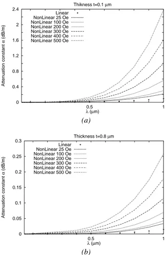
same parameter versus the penetration depth, using the nonlinearity model proposed in Section 2.2.1. In particu-lar, the following cases are considered: (a) t= 0.1 µm; (b) t= 0.2 µm; (c) t = 0.3 µm; (d) t = 0.4 µm; (e) t = 0.8 µm. The peak value of H is assumed in the range 25-500 Oe. It is worth notice that, for low values of the penetration depth, the attenuation constant is similar to that of the linear case and exhibits limited changes in the considered range of H values, for all the t considered. On the con-trary, when the penetration depth increases, the effect of the nonlinearity is rather significant for all t. As expected, the attenuation constant decreases when the thickness of

the superconductors increases. Figure 6.

Figure 6 shows the plot of the attenuation constant ver-sus the penetration depth, which has been obtained by using the model described in Section 2.2.3. In particu-lar, two values of t were assumed: (a) t= 0.1 µm and (b) t= 0.8 µm. The differences between the results of Figure 5 and Figure 6 are very small (less than 0.1% for anyλ and H). The nonlinearity ofλwith respect to H is not very

(10)

significant on the attenuation constant. This confirms the considerations pointed out in [Oates et al., 1991]. The

nonlinearity effects onσ1are much more evident. Fig- Figure 7. ure 7 shows the results for the second-order model

(Sec-tion 2.2.2). In this case, too, we considered (a) t= 0.1 µm and (b) t= 0.8 µm. As expected, the two models predict analogous results for low values of H, whereas for high H levels, notable changes can be noticed and the second-order nonlinearity predicts higher attenuation.

In the second example, a microstrip line made of Y BCO was considered (Figure 2 (b)). The dielectric substrate was made of LaAlO3 (εr = 25) with a thickness d =

500 µm; the width of the signal line was Ws = 150 µm

and the width of the return line was Wgd= 5000 µm. The

above structure is the same as considered in [Liu and Itoh, 1993]. The analysis is performed for different values of the thickness of the superconducting films in the range between 0.002 µm and 0.02 µm. The results are provided

in Figure 8 and correspond to those provided in [Liu and Figure 8.

Itoh, 1993] (Figure 6). Figure 8 shows the values of the attenuation constant for different values of the films thick-ness, and the nonlinearity is modeled as described in Sec-tions (a) 2.2.1 (quadratic nonlinearity), (b) 2.2.2 (cubic nonlinearity), and (c) 2.2.3 (nonlinearity of the penetra-tion depth ), for temperature values of 4K and 77K and assumingλ(0) (linear) = 0.22 µm. As can be seen, for low H, the obtained values are in good agreement with those in [Liu and Itoh, 1993], which have been calcu-lated in the linear case. In the third example, a parallel-plane transmission line (Figure 2 (c)) was considered. As in the previous examples, the superconductor used was Y BCO and the dielectric substrate was made of LaAlO3 (εr= 25). The thickness of the signal and return lines was

t= 0.1µm; the distance was d = 0.1µm and the widths of

the superconductors were Wgd= 150µm. Figure 9.

Figure 9 shows the plots of the attenuation constant versus the penetration depthλ, using the models devel-oped in Sections (a) 2.2.1, (b) 2.2.2. In order to have an idea of the differences in the behaviors predicted by the

two models, Figure 10 shows the attenuation constant Figure 10.

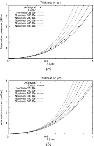
for different values of the penetration depth (in the range 0.1-1 µm) and for two values of the peak H: (a) 25 Oe and (b) 500 Oe. When computed by using the nonlinear model in Section 2.2.3, very small differences (less than 0.05%), have been obtained with respect to the results re-ported in Figure 10 (a). Finally, the same configuration was analyzed, but assuming t= 1µm and d = 1µm. The

results are provided in Figure 11, where, for a consis- Figure 11.

tency check, the values obtained by applying the analyt-ical formulation in [Van Duzer and Turner, 1981] (linear case) are also reported.

(11)

4. Conclusion

The attenuation constant of several superconducting transmission lines widely used in microwave applications has been calculated.

In particular, the experimentally-verified nonlinear be-haviors of superconducting materials at microwave fre-quency has been taken into account. Quadratic and cubic expressions have been used to model the behavior of the superconducting material versus the magnetic field. The significant effect of the nonlinearity on the attenuation constant has been evaluated with reference to a number of configurations and propagation conditions. The im-portance of the modeling of the nonlinear effect clearly resulted from the reported computer simulations.

References

Caorsi, S, A. Massa, and M. Pastorino, Iterative numer-ical computation of the electromagnetic fields inside weakly nonlinear infinite dielectric cylinders of arbi-trary cross sections using the distorted-wave Born ap-proximation, IEEE Trans. Microwave Theory Tech, 44, 3, 400-412, 1993.

Caorsi, S., A. Massa, and M. Pastorino, Numerical Computation of the Interaction Between Electromag-netic Waves and Nonlinear Superconducting Material s, IEEE Trans. Microwave Theory Tech., 2001, in press.

Censor, D., Waveguide and cavity oscillations in the pres-ence of nonlinear media, IEEE Trans. Microwave The-ory Tech., 33, 296-301, 1985.

Censor, D., Harmonic and transient scattering from weakly nonlinear objects, Radio Sci. 22(2), 227-233, 1987.

Choudhury, D. P., B. A. Willemsen, J. S. Derov, and S. Sridhar, Nonlinear response of HTSC thin film mi-crowave resonators in an applied DC magnetic field, IEEE Trans. Appl. Superconduct., 7, 1260-1263, 1997. El-Ghazaly, S., R. Hammond, and T. Itoh, Analysis of superconducting microwave structures: Application to microstrip lines, IEEE Trans. Microwave Theory Tech., 40, 499-508, 1992.

Gupta, K. C., R. Garg, and I. J. Bahl, Microstrip lines and slotlines, Norwood, MA: Arthech House, 1979. Hein, M., et al., Fundamental limits of the linear

mi-crowave power response of epitaxial Y-Ba-Cu-O films, IEEE Trans. Appl. Superconduct., 7, 1236-1239, 1997. Lee, L. H., S. M. Ali, and W. Gregory Lyons, Full-wave characterization of high Tcsuperconducting

transmis-sion lines, IEEE Trans. Appl. Superconduct., 2, 49-57, 1992.

(12)

Lee, H. Y., and T. Itoh, Phenomenological loss equiva-lence method for planar quasi-TEM transmission lines with a thin normal conductor or superconductor, IEEE Trans. Microwave Theory Tech., 37, 1904-1909, 1989. Liu, Y., and Tatsuo I., Characterization of power-dependent hight-Tc superconducting microstrip line by modified spectral domain method, Radio Sci, 28, 913-918, 1993.

Ma, J.-G., and I. Wolff, Electromagnetics in high-Tc su-perconductors, IEEE Trans. Microwave Theory Tech., 44, 537-542, 1996.

Ma, J.-G., and I. Wolff, Electromagnetic behaviour of high-Tcsuperconductors, IEEE Trans. Magnetics., 32,

1160-1163, 1996.

Mei, K. K., and G. Liang, Electromagnetics of super-conductors, IEEE Trans. Microwave Theory Tech., 39, 1522-1529, 1991.

Nguyen, P. P., D. E. Oates, G. Dresselhaus, and M. S. Dresselhaus, Nonlinear surface impedance for Y Ba2Cu3O7−x thin films: Measurements and a coupled-grain model, Phys. Rev. B, vol. 48, 9, 6400-6412, 1993.

Oates, D. E., A. C. Anderson, D. M. Sheen, and S. M. Ali, Stripline resonator measurement of Zsversus Hr f

in Y Ba2Cu3O7−xthin films, IEEE Trans. Microwave Theory Tech., 39, 1522-1529, 1991.

Sheen, D. M., Sami M. Ali, D. Oates, R. S. Withers and J. A. Kong, Current distribution, resistance, and in-ductance for superconducting strip transmission lines, IEEE Trans. Appl. Superconduct., 1, 108-115, 1991. Talanov, V. V., L. V. Mercaldo, and S. M. Anlage,

Mea-surement of the absolute penetration depth and surface resistance of superconductors using the variable spac-ing parallel plate resonator, IEEE Trans. Appl. Super-conduct., 9, 2179-2182, 1999.

Tsuk, M. J., and J. A. Kong, A hybrid method for the cal-culation of the resistance and inductance of transmis-sion lines with arbitrary cross sections, IEEE Trans. Microwave Theory Tech, 39, 8, 1338-1347,1991. Van Duzer, T., and C. W. Turner, Principle of

Super-conductive Devices and Circuits, New York: Elsevier, 1981.

Weeks, W. T., L. L. Wu, M. F. McAllister, and A. Singh, “Resistive and inductive skin effect in rectangular con-ductors,” IBM J. Res. Develop., 23, 6, 652-660, 1979.

(13)

S. Caorsi, Dept. of Electronics, University of Pavia, Via Ferrata 1, 27100 Pavia Italy. (e-mail: caorsi@ele.unipv.it)

M. Donelli, A. Massa, and M. Pastorino, Department Biophysical and Electronic Engeneering, University of Genoa, Via Opera Pia 11A, 16145 Genova Italy. (e-mail: donelli@dibe.unige.it; massa@dibe.unige.it; pas-torino@dibe.unige.it)

(Received January 3, 2001; revised February 27, 2001; accepted March 31, 2001.)

Paper number 01RS2625. 0148-0227/98/98JA-00000$09.00

(14)

CAORSI ET AL.: NONLINEAR EFFECTS IN SUPERCONDUCTING TRANSMISSION LINES

(15)

Figure Captions

Figure 1. Problem geometry. Cross section of the

multi-conducting transmission line.

Figure 1. Problem geometry. Cross section of the multiconducting transmission line.

Figure 2. Nonlinear surface resistance. Experimental

data [Nguyen et al, 1993] and least-square fitting with a second-order nonlinearity (equation (13)).

Figure 2. Nonlinear surface resistance. Experimental data [Nguyen et al, 1993] and least-square

fitting with a second-order nonlinearity (equation (13)).

Figure 3. Superconducting stripline (a),

superconduct-ing microstripline (b) and superconductsuperconduct-ing parallel-plate transmission line (c)

Figure 3. Superconducting stripline (a), superconducting microstripline (b) and superconducting

parallel-plate transmission line (c)

Figure 4. Superconducting stripline. Attenuation

con-stant versus the penetration depthλfor various film thick-ness t (linear case).

Figure 4. Superconducting stripline. Attenuation constant versus the penetration depthλfor various film thickness t (linear case).

con-stant versus the penetration depthλfor various peak val-ues of H and various films thickness t: (a) t= 0.1 µm; (b) t= 0.2 µm; (c) t = 0.3 µm; (d) t = 0.4 µm; (e) t = 0.8 µm (Quadratic nonlinearity (Section 2.2.1)).

Figure 5. Superconducting stripline. Attenuation constant versus the penetration depthλfor various peak values of H and various films thickness t: (a) t= 0.1 µm; (b) t = 0.2 µm; (c) t = 0.3 µm; (d) t= 0.4 µm; (e) t = 0.8 µm (Quadratic nonlinearity (Section 2.2.1)).

(16)

con-stant versus the penetration depthλfor various peak val-ues of H and various films thickness t: (a) t= 0.1 µm; (b) t= 0.8 µm (Quadratic nonlinearity and nonlinearity in the penetration depth (Section 2.2.3)).

Figure 6. Superconducting stripline. Attenuation constant versus the penetration depthλfor various peak values of H and various films thickness t: (a) t= 0.1 µm; (b) t = 0.8 µm (Quadratic nonlinearity and nonlinearity in the penetration depth (Section 2.2.3)).

con-stant versus the penetration depthλfor various peak val-ues of H and various films thickness t: (a) t= 0.1 µm; (b) t= 0.8 µm (Cubic nonlinearity (Section 2.2.2)).

Figure 7. Superconducting stripline. Attenuation constant versus the penetration depthλfor various peak values of H and various films thickness t: (a) t= 0.1 µm; (b) t = 0.8 µm (Cubic nonlinearity (Section 2.2.2)).

Figure 8. Microstrip line. Normalized attenuation

con-stant _ω√α_µ0_ε

0 versus the films thickness t for various peak

values of H and for temperature values of 4K and 77K. Nonlinear cases, modeled as in Sections (a) 2.2.1, (b) 2.2.2, (c) 2.2.3.

Figure 8. Microstrip line. Normalized attenuation constant _ω√α_µ0_ε

0 versus the films thickness t for

various peak values of H and for temperature values of 4K and 77K. Nonlinear cases, modeled as in Sections (a) 2.2.1, (b) 2.2.2, (c) 2.2.3.

Figure 9. Parallel-plane superconducting transmission

line. Attenuation constant versus the penetration depthλ for various peak values of H. Films thickness t= 0.1µm. (a) Quadratic and (b) cubic nonlinearities.

Figure 9. Parallel-plane superconducting transmission line. Attenuation constant versus the

pene-tration depthλfor various peak values of H. Films thickness t= 0.1µm. (a) Quadratic and (b) cubic nonlinearities.

line. Attenuation constant versus the penetration depthλ for the two nonlinear models considered (quadratic and cubic nonlinearities). Film thickness t= 0.1 mum. Peak values of H: (a) 25 Oe and (b) 500 Oe.

pene-tration depthλfor the two nonlinear models considered (quadratic and cubic nonlinearities). Film thickness t= 0.1 mum. Peak values of H: (a) 25 Oe and (b) 500 Oe.

(17)

line. Attenuation constant versus the penetration depthλ for various peak values of H. Films thickness t= 1µm. (a) Quadratic and (b) cubic nonlinearities.

pene-tration depthλfor various peak values of H. Films thickness t= 1µm. (a) Quadratic and (b) cubic nonlinearities.

(18)

Figures

Reference conductor #0 Reference segment Conductor #1 Conductor #M N1i N_1f Nmi N_mf N_0f N0i

Figure 1. Problem geometry. Cross section of the

multi-conducting transmission line.

0 0.1 0.2 0.3 0.4 0 100 200 300 400 500

Surface Resistance Rs (mOhm)

Magnetic Field H (Oe) Experimental T=4.3K Experimental T=46.9K Experimental T=65.6K Calculated T=4.3K Calculated T=46.9K Calculated T=65.6K

Figure 2. Nonlinear surface resistance. Experimental

data [Nguyen et al, 1993] and least-square fitting with a second-order nonlinearity (equation (13)).

(19)

00000000000000000000000 00000000000000000000000 00000000000000000000000 00000000000000000000000 00000000000000000000000 11111111111111111111111 11111111111111111111111 11111111111111111111111 11111111111111111111111 11111111111111111111111 000000000 000000000 000000000 000000000 111111111 111111111 111111111 111111111 00000000000000000000000 00000000000000000000000 00000000000000000000000 00000000000000000000000 11111111111111111111111 11111111111111111111111 11111111111111111111111 11111111111111111111111 x y t d Ws Wgd t (a) 00000000000000000000000 00000000000000000000000 00000000000000000000000 00000000000000000000000 00000000000000000000000 11111111111111111111111 11111111111111111111111 11111111111111111111111 11111111111111111111111 11111111111111111111111 00000000000000000000000 00000000000000000000000 00000000000000000000000 00000000000000000000000 11111111111111111111111 11111111111111111111111 11111111111111111111111 11111111111111111111111000000000000000000 000000000 000000000 111111111 111111111 111111111 111111111 y Ws Wgd d x t (b) 00000000000000000000000 00000000000000000000000 00000000000000000000000 00000000000000000000000 00000000000000000000000 00000000000000000000000 00000000000000000000000 00000000000000000000000 11111111111111111111111 11111111111111111111111 11111111111111111111111 11111111111111111111111 11111111111111111111111 11111111111111111111111 11111111111111111111111 11111111111111111111111 00000000000000000000000 00000000000000000000000 00000000000000000000000 00000000000000000000000 11111111111111111111111 11111111111111111111111 11111111111111111111111 11111111111111111111111 00000000000000000000000 00000000000000000000000 00000000000000000000000 00000000000000000000000 11111111111111111111111 11111111111111111111111 11111111111111111111111 11111111111111111111111 y x Wgd d t (c)

Figure 3. Superconducting stripline (a),

superconduct-ing microstripline (b) and superconductsuperconduct-ing parallel-plate transmission line (c) 0 0.02 0.04 0.06 0.08 0.1 0.1 0.5 1 Attenuation constant α (dB/m) λ (µm) t=0.1 µm t=0.2 µm t=0.3 µm t=0.4 µm t=0.8 µm

con-stant versus the penetration depthλfor various film thick-ness t (linear case).

(20)

0 0.5 1 1.5 2 2.5 0.5 1 Attenuation constant α (dB/m) λ (µm) Thickness t=0.1µm Linear NonLinear 25 Oe NonLinear 100 Oe NonLinear 200 Oe NonLinear 300 Oe NonLinear 400 Oe NonLinear 500 Oe 0 0.5 1 1.5 2 2.5 0.5 1 Attenuation constant α (dB/m) λ (µm) Thickness t=0.2 µm Linear NonLinear 25 Oe NonLinear 100 Oe NonLinear 200 Oe NonLinear 300 Oe NonLinear 400 Oe NonLinear 500 Oe (a) (b) 0 0.1 0.2 0.3 0.4 0.5 0.6 0.7 0.5 1 Attenuation constant α (dB/m) λ (µm) Thickness t=0.3 µm Linear NonLinear 25 Oe NonLinear 100 Oe NonLinear 200 Oe NonLinear 300 Oe NonLinear 400 Oe NonLinear 500 Oe 0 0.1 0.2 0.3 0.4 0.5 0.6 0.5 1 Attenuation constant α (dB/m) λ (µm) Thickness t=0.4 µm Linear NonLinear 25 Oe NonLinear 100 Oe NonLinear 200 Oe NonLinear 300 Oe NonLinear 400 Oe NonLinear 500 Oe (c) (d) 0 0.05 0.1 0.15 0.2 0.25 0.3 0.5 1 Attenuation constant α (dB/m) λ (µm) Thickness t=0.8 µm Linear NonLinear 25 Oe NonLinear 100 Oe NonLinear 200 Oe NonLinear 300 Oe NonLinear 400 Oe NonLinear 500 Oe (e)

con-stant versus the penetration depthλfor various peak val-ues of H and various films thickness t: (a) t= 0.1 µm; (b) t= 0.2 µm; (c) t = 0.3 µm; (d) t = 0.4 µm; (e) t = 0.8 µm (Quadratic nonlinearity (Section 2.2.1)).

(21)

0 0.4 0.8 1.2 1.6 2 2.4 0.5 1 Attenuation constant α (dB/m) λ (µm) Thikness t=0.1 µm Linear NonLinear 25 Oe NonLinear 100 Oe NonLinear 200 Oe NonLinear 300 Oe NonLinear 400 Oe NonLinear 500 Oe (a) 0 0.05 0.1 0.15 0.2 0.25 0.3 0.5 1 Attenuation constant α (dB/m) λ (µm) Thickness t=0.8 µm Linear NonLinear 25 Oe NonLinear 100 Oe NonLinear 200 Oe NonLinear 300 Oe NonLinear 400 Oe NonLinear 500 Oe (b)

con-stant versus the penetration depthλfor various peak val-ues of H and various films thickness t: (a) t= 0.1 µm; (b) t= 0.8 µm (Quadratic nonlinearity and nonlinearity in the penetration depth (Section 2.2.3)).

(22)

0 0.5 1 1.5 2 2.5 3 3.5 0.5 1 Attenuation constant α (dB/m) λ (µm) Thickness t=0.1 µm Linear NonLinear 25 Oe NonLinear 100 Oe NonLinear 200 Oe NonLinear 300 Oe NonLinear 400 Oe NonLinear 500 Oe (a) 0 0.1 0.2 0.3 0.4 0.5 0.5 1 Attenuation constant α (dB/m) λ (µm) Thickness t=0.8 µm Linear NonLinear 25 Oe NonLinear 100 Oe NonLinear 200 Oe NonLinear 300 Oe NonLinear 400 Oe NonLinear 500 Oe (b)

con-stant versus the penetration depthλfor various peak val-ues of H and various films thickness t: (a) t= 0.1 µm; (b) t= 0.8 µm (Cubic nonlinearity (Section 2.2.2)).

(23)

0.0001 0.001 0.01

0 0.01 0.02

Normalized Attenuation Constant

Thikness of thin film t (µm) Linear T=4K NonLinear 25 Oe T=4K NonLinear 100 Oe T=4K NonLinear 300 Oe T=4K NonLinear 500 Oe T=4K Linear T=77K NonLinear 25 Oe T=77K NonLinear 100 Oe T=77K NonLinear 300 Oe T=77K NonLinear 500 Oe T=77K (a) 0.0001 0.001 0.01 0 0.01 0.02

Thikness of thin film t (µm) Linear T=4K NonLinear 25 Oe T=4K NonLinear 100 Oe T=4K NonLinear 300 Oe T=4K NonLinear 500 Oe T=4K Linear T=77K NonLinear 25 Oe T=77K NonLinear 100 Oe T=77K NonLinear 300 Oe T=77K NonLinear 500 Oe T=77K (b) 0.0001 0.001 0.01 0 0.01 0.02

Thikness of thin film t (µm) Linear T=4K NonLinear 25 Oe T=4K NonLinear 100 Oe T=4K NonLinear 300 Oe T=4K NonLinear 500 Oe T=4K Linear T=77K NonLinear 25 Oe T=77K NonLinear 100 Oe T=77K NonLinear 300 Oe T=77K NonLinear 500 Oe T=77K (c)

Figure 8. Microstrip line. Normalized attenuation

con-stant _ω√α_µ

0ε0 versus the films thickness t for various peak

values of H and for temperature values of 4K and 77K. Nonlinear cases, modeled as in Sections (a) 2.2.1, (b) 2.2.2, (c) 2.2.3.

(24)

0 2 4 6 8 10 12 14 16 0.5 1 Attenuation constant α (dB/m) λ (µm) Thickness t=0.1 µm Linear NonLinear 25 Oe NonLinear 100 Oe NonLinear 200 Oe NonLinear 300 Oe NonLinear 400 Oe NonLinear 500 Oe (a) 0 2 4 6 8 10 12 14 16 18 0.5 1 Attenuation constant α (dB/m) λ (µm) Thickness t=0.1 µm Linear NonLinear 25 Oe NonLinear 100 Oe NonLinear 200 Oe NonLinear 300 Oe NonLinear 400 Oe NonLinear 500 Oe (b)

line. Attenuation constant versus the penetration depthλ for various peak values of H. Films thickness t= 0.1µm. (a) Quadratic and (b) cubic nonlinearities.

(25)

0 1 2 3 4 5 6 7 8 9 0.5 1 Attenuation constant α (dB/m) λ (µm) Thickness t=0.1 µm Linear Quadratic nonlinearity Cubic nonlinearity (a) 0 2 4 6 8 10 12 14 16 18 0.5 1 Attenuation constant α (dB/m) λ (µm) Thickness t=0.1 µm Linear Quadratic nonlinearity Cubic nonlinearity (b)

line. Attenuation constant versus the penetration depthλ for the two nonlinear models considered (quadratic and cubic nonlinearities). Film thickness t= 0.1 mum. Peak values of H: (a) 25 Oe and (b) 500 Oe.

(26)

1 2 3 4 5 0.1 0.5 1 Attenuation constant α (dB/m) λ (µm) Thickness t=1 µm Analitycal Linear Nonlinear 25 Oe Nonlinear 100 Oe Nonlinear 200 Oe Nonlinear 300 Oe Nonlinear 400 Oe Nonlinear 500 Oe (a) 1 2 3 4 5 0.1 0.5 1 Attenuation constant α (dB/m) λ (µm) Thickness t=1 µm Analitycal Linear Nonlinear 25 Oe Nonlinear 100 Oe Nonlinear 200 Oe Nonlinear 300 Oe Nonlinear 400 Oe Nonlinear 500 Oe (b)

line. Attenuation constant versus the penetration depthλ for various peak values of H. Films thickness t= 1µm. (a) Quadratic and (b) cubic nonlinearities.