Modelling analysis and implementation of distributed probabilistic timed actors using theatre

Universit´

a della Calabria

DIPARTIMENTO DI INGEGNERIA INFORMATICA, MODELLISTICA, ELETTRONICA E

SISTEMISTICA

Dottorato di Ricerca in

Information and Communication Technologies XXXI ciclo

Modelling Analysis and Implementation of

Distributed Probabilistic Timed Actors

using Theatre

Candidato:

Paolo Francesco Sciammarella

Relatore:

Prof. Libero Nigro

Correlatore:

“That Every long lost dream led me to where you are Others who broke my heart they were like northern stars Pointing me on my way into your loving arms This much I know is true That God blessed the broken road That led me straight to you” Melodie Crittenden - Broken Road

Contents

Preface . . . 7

I Formal Modelling and Verification

9

1.2 Timed Automata Theory . . . 13

1.2.1 Introduction . . . 13

1.2.2 Formal syntax . . . 14

1.2.3 Labelled Transition System semantics . . . 14

1.2.4 Bisimulation . . . 16

1.2.5 Symbolic semantics and Verification . . . 17

1.3 Some Available Model Checking Environments . . . 21

1.3.1 Java PathFinder . . . 21

1.3.2 SPIN and PROMELA . . . 22

2 The Uppaal Symbolic Model Checker 24 2.1 Modelling language . . . 25

2.1.1 Normal, urgent and committed locations . . . 25

2.1.2 Guarded commands . . . 26

2.1.3 Progress conditions . . . 27

2.1.4 Global time and clocks . . . 27

2.2 Query language . . . 28

2.3 Advanced features . . . 29

3 Probabilistic and Statistical Model Checking 32 3.1 Probabilistic Models . . . 33

3.1.1 Discrete-Time Markov Chains (DTMC) . . . 33

3.1.2 Markov Decision Processes (MDPs) . . . 35

3.1.3 Probabilistic Automata (PAs) . . . 36

3.1.4 Continuous-Time Markov Chains (CTMCs) . . . 36

3.1.5 Probabilistic Timed Automata (PTAs) . . . 37

3.2 The Prism probabilistic model checker . . . 38

3.3 Statistical Model Checking . . . 39

3.3.2 Monte Carlo simulations . . . 40

3.3.3 Hypothesis testing . . . 41

3.4 Plasma Lab statistical model checker . . . 46

3.5 VeStA and PVeStA . . . 47

4 The Uppaal Statistical Model Checker 48 4.1 Network of Stochastic Timed Automata . . . 48

4.2 Query language . . . 49

4.2.1 Bound and number of runs . . . 50

4.2.2 Simulation . . . 50

4.2.3 Statistical algorithms . . . 50

4.2.4 Probability Estimation . . . 51

4.2.5 Hypothesis testing . . . 51

4.2.6 Probability comparison . . . 51

4.2.7 Value bound determination . . . 51

4.2.8 Support for WMITL . . . 52

4.2.9 Additional queries . . . 52

4.3 SMC options . . . 53

4.4 Dynamic template processes . . . 53

4.5 Custom probability distribution functions . . . 54

4.6 Non-deterministic vs. stochastic interpretation . . . 55

II Distributed Probabilistic Timed Actors

56

5.2 Timed actors . . . 59

5.3 Actor Extensions for Real Time Modelling and Analysis . . . 61

5.4 The Theatre infrastructure . . . 65

5.4.1 Basic Concepts . . . 65

5.4.2 Programming in-the-small concepts . . . 66

5.4.3 Programming in-the-large concepts . . . 67

5.4.4 Simulation applications . . . 68

5.4.5 Development methodology and model-continuity . . . 68

5.4.6 Implementation status . . . 69

5.4.7 Contributions of this dissertation . . . 69

III Theatre in Action

71

6.2 Related Work . . . 74

6.3 From Modelling to Implementation of a CPS . . . 77

6.3.1 The proposed methodology . . . 77

6.3.2 Control machines and time management . . . 80

6.3.3 Actions and processing units . . . 81

6.3.5 Specializing the envGateway to work with Arduino . . . . 82

6.4 A case study using power management . . . 83

6.4.1 Modelling the system . . . 85

6.4.2 Data configuration . . . 85

6.4.3 Analysis phase . . . 86

6.4.4 Preliminary execution . . . 87

6.4.5 Prototype implementation and real execution . . . 89

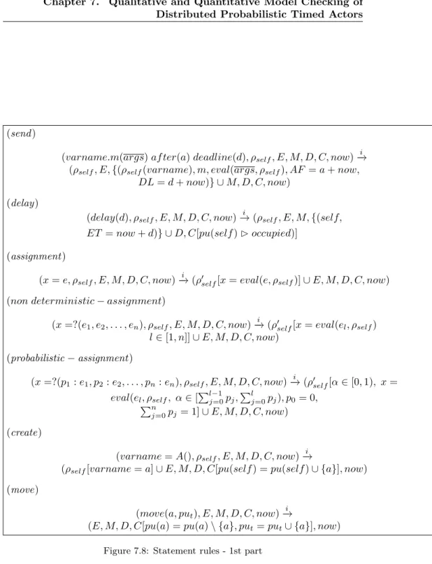
7 Qualitative and Quantitative Model Checking of Distributed Probabilistic Timed Actors 93 7.1 Introduction . . . 93

7.2 THEATRE concepts . . . 96

7.2.1 Architectural view . . . 96

7.2.2 Abstract modelling language . . . 97

7.2.3 A modelling example . . . 98

7.3 An operational semantics of THEATRE . . . 102

7.3.1 Transition rules i ! and! . . . 103d 7.4 A reduction of THEATRE onto UPPAAL . . . 107

7.4.1 Scenario parameters . . . 107

7.4.2 Entity naming . . . 108

7.4.3 Message and delay pools . . . 109

7.4.4 Asynchronous message passing and delay setting . . . 109

7.4.5 Message delivery and arguments . . . 110

7.4.6 The Message automaton . . . 110

7.4.7 Delay automaton . . . 111

7.4.8 An actor automaton . . . 112

7.4.9 Preservation of THEATRE semantics . . . 113

7.4.10 Translated UPPAAL model of the toxic gas sensing system114 7.5 Analysis of a THEATRE model reduced into UPPAAL . . . 116

7.5.1 Qualitative non-deterministic model checking . . . 116

7.5.2 Quantitative statistical model checking . . . 118

7.5.3 Partitioning . . . 124

8 Seamless Development in Java of Distributed Real-Time Sys-tems using Actors 125 8.1 Introduction . . . 125

8.2 An overview of Theatre . . . 125

8.2.1 Basic Java Framework . . . 126

8.2.2 Development Phases And Control Machines . . . 127

8.3 A modelling example . . . 129

8.4 Analysis of the toxic gas system . . . 135

8.4.1 Qualitative Experiments . . . 135

8.4.2 First Scenario: 2 Sensors and Scientist Deadline set to 10 136 8.4.3 Second Scenario: 2 Sensors and Scientist Deadline set to 13137 8.4.4 Third Scenario: 3 Sensors vs. 1 Sensor, 95% Working . . 137

8.4.5 Fourth Scenario: Scientist Die Probability vs. Number of Sensors . . . 138

8.5 Preliminary Execution of the TGS Model . . . 138

8.6 Real time execution . . . 141

8.7.1 Configuration and Bootstrap of a Distributed System . . 143

8.7.2 Actor Migration . . . 145

9 Case Studies 146 9.1 Asynchronous Leader Election . . . 146

9.1.1 Experimental results . . . 148

9.2 A Time Synchronization Algorithm . . . 148

9.2.1 Modelling the Time-Synch algorithm using Theatre . . 151

9.2.2 Experimental results . . . 153

9.3 Actor-based NetBill Protocol . . . 159

9.3.1 Modelling the NetBill protocol into Uppaal SMC . . . . 161

9.3.2 Experimental results . . . 162

10 Modelling and Analysis of Multi-Agent Systems Using Uppaal168 10.1 Introduction . . . 168

10.2 Modelling the Iterated Prisoner’s Dilemma . . . 169

10.2.1 Case study description . . . 170

10.2.2 An IPD actor-based model . . . 171

10.3 A structural translation from actors to Uppaal SMC . . . 172

10.3.1 Actor and message naming . . . 173

10.3.2 Dynamic messages . . . 173

10.3.3 Actor automata . . . 175

10.3.4 Other global declaration . . . 176

10.4 Experimental work . . . 178

10.4.1 Debugging queries . . . 178

10.4.2 Transient behavior . . . 179

10.4.3 Emergence of cooperation in the scenario-1 . . . 180

10.4.4 Emergence of cooperation in the scenario-2 . . . 181

10.4.5 Model validation . . . 184

11 Conclusions 186 12 List of publications and bibliography 188

IV Appendixes

212

A.2 The formalism of Stochastic Time Petri Nets . . . 214

A.2.1 Basic Concepts . . . 214

A.2.2 Syntax . . . 214

A.2.3 Semantics . . . 215

A.3 Mapping sTPN onto Uppaal . . . 216

A.3.1 Timed Automata For Transitions . . . 217

A.4 First Example . . . 219

A.5 Experimental analysis . . . 221

A.5.1 Non-deterministic analysis . . . 221

A.6 Second Example . . . 226

A.7 Analysis of the Fisher’s protocol . . . 227

A.7.1 Non-deterministic analysis . . . 229

A.7.2 Stochastic Analysis . . . 230

A.8 Conclusions . . . 232

B A layered IoT-based architecture for distributed SHM 234 B.1 Introduction . . . 234

B.2 SHM Based On Multi-Agent IoT . . . 235

B.2.1 Sensing layer . . . 237

B.2.2 Signal Processing Layer . . . 239

B.2.3 Event Detection Layer . . . 239

B.2.4 Application Layer . . . 240

B.2.5 Remote Transmission Protocol . . . 241

B.2.6 Experimentation validation . . . 242

C Acknowledgements 246

Preface

Nowadays, the technological advances introduced e.g. by the Internet-of-Things, motivate the development of complex software systems, which can exploit the growing connection flexibility among different computational units and devices. Smart objects, embedded systems and cyber-physical systems are just a few examples of design techniques and applications fueled by this ongoing techno-logical revolution.

From a software engineering point of view, systems that follow these design methods and operation logic, are best known as reactive systems. Reactive systems are computer systems that continuously react to the external stimuli generated by the user or by a controlled environment, producing an answer as soon as the request arrives. Such systems cover different safety and business critical areas such as e-commerce, e-banking, air traffic control, mechanical de-vices control for train operation or nuclear reactors and many others.

Correctness and reliability are project requirements of paramount importance in the design of many of the above mentioned systems. In fact, an application failure or malfunction can have severe consequences from the practical point of view.

Traditional software validation techniques are simulation and testing. Unfortu-nately, they are insufficient because not exhaustive. They are often manually constructed and typically can explore only a small fraction of all the possible computational paths. Therefore, they cannot guarantee the absence of bugs in the left unexplored state trajectories, particularly in the presence of complex concurrent interleavings.

In the last few decades, the alternative approach of formal verification emerged, which is based on the exhaustive exploration of all the possible system behav-iors. Using e.g. the model checking technique, it is possible to determine if a (not large) system satisfies a specific behavioral property, by examining all its reachable states. However, with not trivial systems, model checking can incur into the state explosion problem which limits its practical applicability. A more approximate solution to infer properties and ensure system correctness, is based on the concept of statistical model checking. It uses a finite number of system executions and hypothesis testing, to judge if collected samples provide a sta-tistical evidence for the specification satisfaction or violation.

This thesis is devoted to developing methods and tools of software engineer-ing, supporting modellengineer-ing, analysis and implementation of reactive systems.

What makes the development of such systems very challenging is the neces-sity of handling in combination such issues as distribution, non-determinism, probabilistic/stochastic behavior, concurrency, timing constraints, heterogene-ity, synchronicity and asynchronicheterogene-ity, which can render systems undecidable. The Actors computational model is widely recognized as a reference point for building reactive systems. It relies on highly modular encapsulated entities which interact to one another by asynchronous message passing. Extensions have been proposed to actors so as for them to be more adapt for distributed probabilistic real-time systems. A notable project on timed and probabilistic actors is represented by the family of Rebeca modelling languages and related analysis tools based on McErlang, PRISM and recently IMCA.

Starting from some previous research carried out in the Software Engineering Laboratory (www.lis.dimes.unical.it), directed by Prof. Libero Nigro, the pro-posed work consists in enhancing a lightweight actor system called Theatre, so as to provide a formal modelling language in the light of the inspiring Re-beca work, together with some supporting tools for property assessment which in a case are based on the Uppaal model checkers (qualitative analysis - detect-ing that an event can occur - based on the non-deterministic exhaustive model checker, and quantitative analysis - finding a quantitative measure of the prob-ability for an event to actually occur- based on the statistical model checker). An important part of the work consists in experimenting the use of Theatre according to the concept of model continuity, namely transitioning, without dis-tortions, a same model from early analysis down to design, prototyping and final implementation in Java. The goal is trying to ensure faithfulness of a synthe-sized system to the analyzed model.

The accomplished work on Theatre is accompanied by several concrete appli-cations and case studies aimed at demonstrating the flexibility and potential of Theatre features.

The thesis is structured in three parts. In the first part (chapters from 1 to 4), the concepts of formal modelling and verification are summarized. In partic-ular, the automated techniques of exhaustive symbolic model checking, based on timed automata, and of probabilistic and statistical model checking are dis-cussed. As a notable example, the Uppaal model checkers, used in this thesis, are outlined. In the second part (chapter 5), the development issues of dis-tributed probabilistic and timed actor systems are reviewed, together with some relevant related works. All of this provides context for the Theatre actor sys-tem which is the goal of this thesis. Moreover, the contributions of this work are highlighted. In the third part (chapters from 6 to 10), the main developments and achievements concerning the extended version of Theatre, its implemen-tation in Java and its application to modelling and verification of selected case studies are described. The thesis terminates by presenting conclusions and by furnishing directions of future works. Two appendixes complete the dissertation which refer to some additional accomplished work: that of experimenting with modelling and analysis of Stochastic Time Petri Nets and showing a further ap-plication of our actors to a prototypical structural health monitoring and control system.

Part I

Formal Modelling and

Verification

Chapter

1

Concepts of Model Verification

The development of reliable hardware and software systems is a well-known critical and crucial issue [83]. In the last decades, several tools have been devel-oped to help to identify defects and implementation problems. Although very often used, simulation and testing techniques [28, 133, 169] prove inadequate for correctness assessment [94]. As shown in Fig. 1.1, testing normally works by comparing results obtained at run-time, with the expected ones computed on a finite set of test-cases [176]. Only a small fraction of all the computational paths is investigated. Moreover, by using a few runs, problems such as dead-locks or concurrency errors due to complex thread interleavings, are not easily reproducible or detectable [261].

Figure 1.1: Schematic view of the testing workflow

Formal verifications methods [125], based on mathematical techniques, aim to prove the correctness of a system by reasoning on an abstract model and carrying an exhaustive exploration of all the possible reachable configurations [166](see Fig. 1.2. Such methods combine three main components [171], that are:

• an abstract model, that is in charge of emulating the system behaviour; • a specification language, used to formally express system requirements and

properties of interest;

• an analysis method, that is in charge to verify the fulfilment of the require-ments.

Modelling is a creative yet difficult activity [162] which involves experience and abstraction, that is introducing only relevant details while omitting non-essential

Chapter 1. Concepts of Model Verification others. This work claims, though, that a model should facilitate subsequent transitioning of a model toward the design and final implementation phases. In other words, modelling should be not so much abstract but it should admit such issues as distribution/concurrency, probabilistic and timing aspects. By reducing the semantic gap between modelling and synthesis, the goal is to ensure to the large extent “faithfulness” of an implementation to its analyzed model [235].

Several approaches to formal verification are nowadays available such as model checking [25], that is a widespread and mostly studied technique to automate properties verification. It differs, e.g., from theorem provers [40], which require first a (possibly complex) mathematical formalization of the problem but not always offer the possibility of checking timing properties.

Figure 1.2: Correctness verification by using testing or exhaustive exploration, taken from [172]

1.1 Model Checking

Model checking was independently developed by Clarke and Emerson [81] and Queille and Sifakis [214]. As shown in Fig 1.3 the starting points to perform this procedure relies on two components:

• a formal description M of the model under analysis;

• a logical property ' associated with a requirement that has to be evaluated, written in a specification language, like classical computational tree logic (CTL) [81], linear temporal logic (LTL) [211] and their extensions. If the given model satisfies the logical property, we write that M |= ', on the contrary we write M 6|= ', and the model checker suggests a diagnostic trace (counterexample), practically a path of event occurrences, where the violation takes place.

During verification the model checker compiles the model under investigation into a directed state-transition graph, called Kripke structure [139], consisting of:

Chapter 1. Concepts of Model Verification

Figure 1.3: Schematic view of the model checking workflow

• edges, which represent transitions between states, i.e., events that are in charge of changing the system status.

More formally, a Kripke structure over a set A of atomic propositions (i.e. boolean expressions), is a triple K = hS, R, Li where:

• S is the state-space that includes all the possible states as a set of true atomic propositions, where s0 is the initial state;

• R ✓ S ⇥ S is the transitions set;

• L : S ! 2A _{is the labelling function that associates a set of valid atomic}

propositions to each state. In particular, the notation L(s) groups together the true propositions for the system, when it is in the state s [84].

Figure 1.4: Example of a state graph

A model checker can explore the entire state space of a system, evaluating all the possible computational paths in order to verify if a property is satisfied. The model checking theory, though, has a computational limit due to resources needed in terms of time and memory for verification. When analyzing non-trivial medium-large sized systems, in fact, the number of computational paths tends to increase exponentially, even after adding a single variable. This leads to the construction of a huge state graph, which cannot possibly be completed. The problem, known as the state-space explosion, limits the use of model check-ers and has committed researchcheck-ers to an attempt to identify alternatives or optimizations, such as symmetry reduction [99] or partial order reduction [83].

Chapter 1. Concepts of Model Verification

Figure 1.5: Timed Automata and Location Invariants, taken from [31]

1.2 Timed Automata Theory

Among the different modelling languages available to design systems, such as Time Petri Nets [35], timed process algebras [219] [182], and real-time logics [262], in this work the timed automata formalism was chosen, because it con-stitutes the core of the input language used by Uppaal, that is the symbolic model checker exploited for the verification.

1.2.1 Introduction

Timed automata (TA) [16] are an extension of the finite-state Büchi automata, enriched with a set C of real number variables called clocks [27]. Intuitively, TA are finite-state machines with clocks used to model the time elapse, accord-ing to a dense-time notion. All the clocks values are initialized to zero, and increased synchronously with the same rate. They and may be reset during an execution path. A transition edge may be labelled with a guard, consisting of a time-constraint belonging to the set B(C) of all the possible constraints built over the clocks C, and a set of actions ranging over a finite alphabet ⌃. A guard has the form x ⇠ k or x y ⇠ k, where x, y 2 C are clock variables, k is a non-negative integer and the operator ⇠2 {, <, ==, >, }, and its fulfilment enables the edge and, if the transition is taken, the corresponding action is car-ried out.

Figure 1.5 a) depicts an example of timed automaton, taken from [31]. Its timed behavior depends on the value of two clocks: x, that is used to control the self-loop in the location loop, and y, that is used to control the time elapse of the overall model. The dynamic progress is as follow. At the beginning, the automaton may leave the location start at any time when the y value is in the interval [10, 20]. Then it may evolve towards the loop place, along with the self-loop if x==1, and finally it can move to end when y is in [40, 50]. After that, since the y value is reset, the automaton may return to start when the y is in [10, 20]. In the TA, satisfaction of a guard on an edge is a necessary but not sufficient condition for moving from one location to another. In the example in figure 1.5 a), the automaton may stay forever in any location.

Chapter 1. Concepts of Model Verification To ensure progress, in [16] the Büchi acceptance condition was introduced, that is marking a set of locations as accepting, and having that the only admissi-ble automaton executions are those that include an infinite transit from them. Marking in figure 1.5 a) the location end as accepting, it would imply that all the automaton executions must visit that location infinitely times, thus ensur-ing progress. As a consequence, the location start will be left at most when y == 20; would this not happen, the acceptance condition would be violated, because after 20 the guard on the edge becomes invalid and the automaton will be blocked in that location. A similar argument could be applied to the loop location.

A simpler and more intuitive notion of progress was introduced in the Timed Safety Automata [31]. Clock constraints in the form x ⇠ k, called invariants, are used to label locations and give them a local view of time behaviour. An au-tomaton can remain in a location as long as its invariant is satisfied, and forced to exit when the invariant is up to be violated. Would no output transition be enabled, a deadlock will occur. In figure 1.5 b) an example is shown.

In literature, Timed Automata and Timed Safety Automata most often denote the same concept.

1.2.2 Formal syntax

Formally, a timed automaton is a tuple (L, l0, C, A, E, I), where:

• L is a finite set of locations; • l02 L is the initial location;

• C is the set of clocks;

• A is a set of actions (i.e. the alphabet ⌃);

• E ✓ L ⇥ A ⇥ B(C) ⇥ 2c_{⇥ L is a set of edges between locations with an}

action, a guard and a set of clocks to be reset;

• I : L ! B(C) is a function that assigns invariants to locations.

An edge is also indicated as l g,a,r! l0_{2 E where g is a guard, a is an action, r}

is a set of clocks to reset.

To analyze concurrentcy systems modelled as a network of interacting TA, TA theory rests on the product automaton built using the CCS parallel composi-tion operator [177]. Although this operacomposi-tion is entirely syntactical and allows interleaving of actions as well as hand-shake synchronizations, it has a com-putationally expensive cost. For this reason tools such as Uppaal, generate on-the-fly the product automaton during verification. Figure 1.6 depicts some examples of timed automata composition. The notation associated to the case c), i.e., the symbols ! and ? modelling hand-shake synchronization, will be clar-ified below.

1.2.3 Labelled Transition System semantics

For verification of a single timed automaton, the model checker works on a state-graph which is a labelled transition system (LTS), directly corresponding

Chapter 1. Concepts of Model Verification

Figure 1.6: Examples of product automaton: a) sychronous composition, b) asyn-chronous composition, c) explicit synchronization composition

to the operational semantics of the automaton. A LTS consists of a collection of states and transitions. A state is a pair (l, u) 2 L ⇥ RC_{, where l is a location id}

and u is a clock valuation (u 2 R+). A state represents a specific configuration

of the model in which a set of predicates pi 2 P hold. The initial state s0 of a

LTS is (l0, 0|C|). Transitions denote all the possible ways an LTS state has to

evolve. They are labelled with actions ai2 A, executed when the transition is

taken [247].

Formally, let A and P be sets of actions and predicates respectively. A LTS over A and P is a triple (S, !, |=), where:

• S is a set of states;

• ! is a set of transitions !✓ S ⇥ ⌃ ⇥ S, where ⌃ = Ra +

[ {d} is the set of moves [213];

• |=✓ S ⇥ P , indicates that a predicate p 2 P holds in state s 2 S.

To infer properties, all the possible LTS reachable paths need to be explored and evaluated.

The transitions of a LTS can be of two types:

• a delay transition, labelled with a real number, which expresses the possi-bility for an automaton to stay for a certain time d in a state, as long as ddoes not violate the invariant:

(l, u)_{! (l, u + d) if (u + d) 2 I(l) for any d 2 R}d +

• an action transition, labelled with elements of ⌃, which expresses the possibility for an automaton to evolve towards another state, following an enabled edge and possibly resetting a subset of clocks:

(l, u)! (la 0_{, u}0_{)if l} g,a,r_{! l}0_{, u 2 g, u}0_{= [r7! 0]u and u}0_{2 I(l}0₎

A timed action is a pair (t, a), representing an action a 2 ⌃ executed by an automaton after t 2 R+time units since the beginning of the run, where t is the

absolute time, or time-stamp of the action a. A sequence (possibly infinite) of timed actions of an automaton ⇠ = (t1, a1)(t2, a2) . . . (ti, ai) . . ., where ti ti+1

Chapter 1. Concepts of Model Verification for all i 1, is a timed trace. A run of an automaton in the corresponding LTS, with initial state (l0, u0)and over a timed trace ⇠ = (t1, a1)(t2, a2)(t3, a3) . . ., is

defined as a sequence of transitions: (l0, u0) d1 !a1 ! (l1, u1) d2 !a2 ! (l2, u2) d3 !a3 ! . . . where ti= ti 1+ di for all i 1.

The semantics of a network of TA is the associated LTS generated from the product automaton, and it is similar to that a single automaton. To model hand-shake synchronizations (see Figure 1.6), the action alphabet ⌃ is assumed to consist of symbols for input actions denoted a?, output actions denoted a!, and internal actions represented by the distinct symbol a.

The state of a LTS associated to a network of TA is a pair (l, u), where l = l1, l2, . . . ,n is a vector constituted by the current locations of each automaton of

the network and u is a clock array that summarizes the current values of clocks of the system. The rule for delay transitions is similar to the case of a single automaton, where the invariant of a location vector is the conjunction of the location invariants of the processes.

Let listand for the i th element of a location vector l and l[l0i/li]for the vector

l with li being substituted with li0. The transition rules are defined as follows:

• (l, u)! (l, u + d) if u 2 I(l) and (u + d) 2 I(l), where I(l) = ^I(ld i)

• (l, u)! (l[la 0 i/li], u0)if li g,a,r ! l0 i,u 2 g, u0 = [r7! 0]u, u02 I(l[l0i/li]) • (l, u)! (l[la 0

i/li][lj0/lj], u0)if there exist i 6= j such that:

– li gi,a?,ri ! l0 i, lj gj,a!,rj ! l0 j and u 2 gi^ gj, and – u0_{= [r}

i[ rj 7! 0]u and u02 I(l[l0i/li][l0j/lj])

where u0 _{is obtained by resetting a subset of clocks.}

It is important to note that a network is a closed system, which may not perform any external action [31].

1.2.4 Bisimulation

The set of the all finite timed traces of a LTS A is denoted by L(A) and is called the timed language of A. Two different LTSs A1 and A2 are

timed-language equivalent if and only if L(A1) =L(A2). In order to check behavioural

equality among processes, language equivalence is not the most suitable notion to consider. Bisimulation equality, called bisimilarity, among different states within a LTS or different LTSs, is the most used technique to determine and check behavioural similarities [226].

Let (S, !, |=) be an LTS over A and P . A bisimulation is a binary relation R ✓ S ⇥ S over the set of states, satisfying:

• if s1R s2 then s1|= p , s2|= p for all p 2 P ,

• if s1R s2 and s1! sa 01with a 2 A, then there exists a transition s2 ! sa 02

such that s0 1R s02,

Chapter 1. Concepts of Model Verification • if s1R s2 and s2

a

! s0

2with a 2 A, then there exists a transition s1 a

! s0 1

such that s0 1R s02.

Two states s and s0 _{are timed bisimilar, written as s ⇠ s}0_{, if and only if there is}

a timed bisimulation that relates them.

Let g = (S, I, !, |=) and h = (S0_{, I}0_,!0_,|=0_{)be process graphs over A and P . A}

bisimulation between g and h is a binary relation R ✓ S ⇥ S0_{, satisfying I R I}0

and the same three clauses above. g and h are bisimilar, written as g ⇠ h if there exists a bisimulation between them [247].

Figure 1.7: Example of two processes not bisimulation equivalent, taken from [247] Figure 1.7 shows an example of two not bisimulation equivalent processes, taken from [247]. They accept the same language, but the choice between b and c is made at different moment, because the two systems have different branching structure.

Intuitively two systems are considered bisimilar if they match each other’s moves, becoming indistinguishable from an observer. More details can be found in [208] and [167].

1.2.5 Symbolic semantics and Verification

The reachability analysis, performed on the LTS generated from a network of TA, is a key problem in verification, because the correctness of a model can be verified starting from a question: a given desirable or undesirable state of the model is reachable from its initial state [181]? Two class of algorithms can be applied to answer this question, performing:

• the forward analysis, that consists of computing iteratively the successors of the initial states and checking if the state we want to reach is eventually computed or not;

• the backward analysis, that consists of computing iteratively the predeces-sors of the states we want to reach and of checking that the initial state is eventually computed or not.

Since to medium-sized network of TA, can be associated LTSs containing an uncountable set of reachable states, such analysis can be difficult or not decid-able. This is due to the fact that in a state (l, u), u represents an instantaneous evaluation clocks. Such time granularity originates a potentially infinite state-space, because locations with a same data part, will be included in several states which are distinguished each other only by the potentially different infinite in-stantaneous clock values. This limit can be overcome by partitioning the clocks evaluations by a finitely equivalence relation. Exploiting the concept of time abstract bisimulation, by which two configurations s and s0 _{are equivalent when}

Chapter 1. Concepts of Model Verification any action transition a (or any delay transition d) enabled by s, can be simu-lated from s0_{by an action transition a (or a delay transition d}0_{), it is possible to}

compact the representation [181]. In a LTS two configuration states (l, u) and (l0, u0), can be considered equivalent if l = l0 and if u ⌘M u0, i.e., if:

• they exactly satisfy the same clock constraints of the TA;

• in both automata the time elapse, will lead to same integer values for the clocks, in the same order [181].

where M is the maximal constant value appearing in the guards of the automa-ton associated to the specific clock. Using the notation u ⌘M u0 holds whenever

for each clock x 2 X,

• u(x) > M , u0_{(x) > M,}

• if u(x)  M, then bu(x)c = bu0_{(x)c, and ({u(x)} = 0 , {u}0_{(x)} = 0),}

where the operator b↵c indicates the integer part of ↵, while {↵} the fractional part,

and for each pair of clocks (x, y),

• if u(x)  M and u(y)  M, then {u(x)}  {u(y)} , {u0_{(x)}  {u}0_(y)}.

The relation ⌘M is called region equivalence and the associated equivalence class

is called a region [15]. States placed within the same region will always evolve into states belonging to the same region and this feature enables to characterize (and reduce) the state-space of a LTS in terms of a finite region automaton or region graph RA. The RAcan be built starting from the initial LTS A and the

equivalence relation, following this formal semantics:

• states of the graph are pairs (l, R) where l is a location of LTS and R is a region;

• the transitions are expressed by (l, R)! (la 0_{, R}0_{)if there exists a transition}

l g,a,r_{! l}0 _{in A, a valuation v 2 R and d 0 such that u + d |= I(l),}

u + d_{|= g, [r 0](u + d) |= I(l}0_{)and [r 0](u + d) 2 R}0_.

The region graph size depends exponentially from the number of the involved clocks and the maximal constant parameter value appearing in the guards. This means that these parameters may lead to state explosions, because a large num-ber of configurations (arising from all the possible regions), needs to be checked. As reported in [31], figure 1.8 depicts an example of all the admissible regions for an automaton with two clocks x and y, where the x maximum value is 3, while the y maximum value is 2. All corner points (intersections), line segments, and open areas are regions. Doing maths, the number of possible regions in each location is 60. The fundamental property of RA is that it recognizes exactly

the set of words a1a2. . . if exists a corresponding timed word (a1, t1)(a2, t2) . . .

recognized by A. This allows to check a reachability property of a location in A, by resolving a reachability problem in its RA.

In figure 1.9 it is showed an example of a LTS A and of its own region automa-ton RAtaken from [17]. As one can see, the location l3 of A is reachable if and

only if one of the states (l3, R) with a region R is also reachable in RA. By

Chapter 1. Concepts of Model Verification

Figure 1.8: Example of regions

(l3, 0 < y < x < 1) leads to l3. Consequently, this implies that in A exists an

execution, given by (l0, u0) t1 ! (l0, u0+ t1) a ! (l1, u1) t2 ! (l1, u1+ t2) c ! (l3, u2),

that leads to l3, identifiable for some value of t1and t2.

Figure 1.9: a) A labelled transition system A b) The corresponding region graph RA. Example taken from [17]

In practice, model checker tools avoid the construction of the region automaton, because the region partition is too refined and not efficient to be manipulated. To provide a more efficient representation of the symbolic state-space, in [41] the concept of zone and zone-graph was introduced, that rely on the concept of on-the-fly algorithms. A zone is defined as the solution set of a conjunction of atomic clock constraints, among inequalities of the form:

xi xj  uij, li xi ui

where i, j 2 {1, . . . , n} and uij, li, ui 2 R. Compared with regions, zones offer

a more coarse and reduced representation of the state-space [96]. In fact, the symbolic states of a zone graph that would be manipulated by the forward and backward analysis algorithms, are defined by (l, Z), where Z 2 B(C) is a zone defined through the union of clock constraints, that incorporates several

Chapter 1. Concepts of Model Verification

Figure 1.10: Example DBM taken from chapter 4 of [181]

symbolic states of the region graph, having the same data part and satisfying the same time constraints.

Many operations can be performed using this representation [181], that simplify the implementation of algorithms useful for testing reachability.

Zones are efficiently represented and stored in memory by Difference Bound Matrices (DBMs) [30], that are (n + 1)-square matrices, where n is the number of clocks. Coefficients (mi,j)0i,jnof a DBM M are pair of values (k, ), where

kis an integer and is either < or , representing the constraint xi xj ki,j,

involving the set of clocks {xi| 1  i  n}. Moreover, to represent a constraint

in the form xi k a fictitious clock x0is introduced, whose value is always 0; so

it is possible to write mi,0= kwith the associated constraint xi x0 k. Using

an example taken from chapter 4 of [181], in figure 1.10 the zone defined by the constraint (x1 3)^ (x2 5) ^ (x1 x2 4) can be represented through the

matrix of the coefficients M. The presence in a cell of the +1 value indicates that there is no constraint between the clocks associated to the specified row and column, while a negative coefficient is used to model a constraint, in fact, considering m0,1 = 3, the original constraint x1 3 can be modelled

equivalently as x0 x1 3.

Despite every DBM represents a zone, and every zone can be represented by a DBM, the correspondence is not unique and a same zone can be represented by several DBMs.

In order to reduce the computing cost of a DBM, alternative solutions known in literature are minimization algorithm for DBMs [156], federations [87] that are in charge to merge efficiently DBMs or clock difference diagrams (CDDs) [155].

Zones are also related to regions through the following properties: • each region is a zone;

• if Z is a zone, then Z =Siri, where each ri is a region;

• if W =SiZi is convex and each Zi is a zone, then W is a zone.

To better understand the concept of zone, an example taken from [75] is shown in figure 1.11. The model describes a simply timed automaton of a periodic task, whose period is 6 time units. Each task instance consists of two sequential actions, having a not deterministic duration in the range [1, 3] and [2, 3] respec-tively. Locations L0 and L1 model action execution, while L2 is used to model

the waiting period of the next task activation. Two clock variables are used: x that is in charge to measure actions duration and y that is used to measure the periodic behaviour. In order to ensure the non-deterministic attendance, invari-ant conditions coupled with appropriate guards are introduced such as x  3 attached to L0 and x 1 on the output edge from L0 to L1. Some edges are

Chapter 1. Concepts of Model Verification

Figure 1.11: a) A simple of periodic timed automaton b) Associated zone state graph equipped with clocks resetting actions, needed to allow the correct measure of the sojourn time. For example, on the edge from L2 to L0 the values of both

clocks are set to zero, to indicate the beginning of a new instance of the task and to count the flow of other 6 time units, while on the edge from L0 and L1

x, is reset to measure the duration of the second action.

While the zones for the locations L0 and L1 are identifiable in an easy way, the

clock constraints on L2 are not obvious and need to be clarified. On L2 the

constraints are 2  x  5 and 3  y  6, because in the best case L2 can be

reached after the sum of 1tu needed to leave L0 and 2tu to exit from L1 on y,

but after 2tu on x due to the x reset from L0 to L1, while the upper bounds

can be immediately calculated. Considering the difference y x, doing maths, it is deduced that 1  y x_{ 3, where 1 = y} x and y x = 3, that are respectively the remaining lines used to delimit the zone.

1.3 Some Available Model Checking Environments

Besides Uppaal, several tools are currently available (and constantly evolving), useful for making model checking. In this section, a few of them are summarized.

1.3.1 Java PathFinder

Java PathFinder (JPF) is a model checker that has been developed as a verifica-tion and testing environment for Java multithreaded programs [172]. It is open source and online available and consists of a custom-made Java Virtual Machine (JVM) that is in charge to execute a program (Java bytecode) not only once as a normal VM, but theoretically in all the possible ways, exploring thread inter-leaving and non-deterministic assignments, for checking property violations like deadlocks or unhandled exceptions. For properties specification JPF uses:

• Java assertions inside the application under analysis (in this case any violation is captured and notified to the user);

• instance of gov.nasa.jpf.Property, gov.nasa.jpf.GenericProperty, or through the implementation of two listener classes gov.nasa.jpf.SearchListener and

Chapter 1. Concepts of Model Verification

Figure 1.12: Java PathFinder architecture, taken from [172] gov.nasa.jpf.VMListener.

JPF cannot analyze Java native methods and if the system under test calls such methods, these have to be provided within peer classes or intercepted by listeners.

The two main features of JPF are:

• backtracking, which indicates the ability to restore previous execution states, to see if there are unexplored choices left;

• state matching, during the execution a match is made between a new reached status and any other previously examined. JPF can then back-track to the nearest non-explored non-deterministic choice.

Like other model checkers, also JPF is prone to state-explosion problems. Since concurrent actions can be executed in any arbitrary order, all their possible interleavings can lead to a very large state space. In particular, for n threads with m statements each, the number of possible scheduling sequences is equal to:

K = (nm)!

m!n (1.1)

JPF model checking can purposely exploit two techniques:

• state abstraction, which eliminates details irrelevant to a property, obtain-ing a simple finite model sufficient to verify the property. It can produce false positives/negatives due to the loss of precision;

• Partial Order Reduction (POR) which basically groups all instructions in a thread, that do not have any effects outside the thread, into a single transition.

Other detail can be found in [42], [172] and [207].

1.3.2 SPIN and PROMELA

SPIN is a popular open-source model checker, that can be used for formal veri-fication of multi-threaded applications and for analyzing the logical consistency of concurrent and distributed systems [123].

Chapter 1. Concepts of Model Verification The tool supports a high-level modelling language called PROMELA (PROcess MEta LAnguage), which allows the creation of processes by using classical data types, control flow instructions, loop structure, atomic statements, complex data structures, and process communication through the use of shared memory or message channels that can be synchronous (i.e., rendezvous), or asynchronous (i.e., buffered).

SPIN has been used to trace logical design errors in distributed systems design, such as operating systems, communications protocols, switching systems, con-current algorithms, railway signalling protocols, control software for spacecraft, nuclear power plants, etc. highlighting the presence of deadlocks, race condi-tions, different types of incompleteness, and unwarranted assumptions about the relative speeds of processes. Moreover, that tool directly supports the use of embedded C code as part of model specifications and using the model extractor modex, it is also possible to automatically generate a PROMELA model from a concurrent C code.

SPIN enables the use of multi-core computers for model checking, supporting the verification of both safety and liveness properties. It works on-the-fly, avoid-ing the need to preconstruct a global state graph, thus makavoid-ing it possible the checking of large system models. Property specification can be based on LTL, but other alternative and efficient on-the-fly ways, for safety and liveness verifi-cation exist. Correctness properties can also be specified as a system or process invariants (using assertions) and as formal Büchi automata.

Spin can be used in four modalities:

• as a simulator, that allows a rapid prototyping of the model under inves-tigation;

• as an exhaustive verifier, to demonstrate the validity of user-defined re-quirements (using partial order reduction to optimize the search); • as proof approximation system, that can validate very large system models,

covering the maximum state space available;

• as a driver for swarm verification, which can make optimal use of large numbers of computing cores, to detect defects in large models.

All Spin software is written in ISO-standard C, and is portable across all versions of Unix, Linux, cygwin, Plan9, Inferno, Solaris, Mac, and Windows.

Chapter

2

The Uppaal Symbolic Model

Checker

Uppaal is a popular, online available, continuously evolved, symbolic model checker jointly developed by the Uppsala University and the Aalborg University. It runs on the most common operating environments: Windows, Linux, Mac OS. It is designed for the exhaustive verification of real-time systems modelled as networks of timed automata (TA) [27]. Compared to similar tools, such as HyTech [117] and Kronos [266], Uppaal is characterized by the adoption of compact data structures to represent the state graph of a model, and efficient traversal algorithms.

The main features of Uppaal which motivated its use in this work are: • its high expressive and simplicity of modeling, through the use of a

user-friendly GUI;

• its faster verification engine;

• its extension with a statistical model checker.

In the past, Uppaal was successfully exploited for off-line verification of in-dustrial protocols, such as the collision handling in the Philips Audio Control Protocol (PACP) [38]. More recently, it was applied, e.g., to the on-line op-timization of home automation and traffic control systems [157], such as the Intelligent Control of Traffic Light (ICTL) [100], or the CASSTING project, where the tool is used to synthesize an improved controller for a floor heating system of a single family house [154].

The toolkit is composed by three sub-environments:

• an intuitive graphical front-end editor, written in Java, used to design a TA model;

• a simulator, which allows to animate a model in order to observe graphi-cally its execution;

• a verifier or server, written in C++, that implements the model checking engine which generates the state-graph of a model and verifies the satisfac-tion of the property queries of interest. The verifier is able to analyze all

Chapter 2. The Uppaal Symbolic Model Checker the possible interleavings among the actions of the concurrent component processes.

This chapter briefly reviews the Uppaal symbolic model checker by focusing on the modelling capabilities and the query specification language.

2.1 Modelling language

The Uppaal modelling language extends the classical timed automata formal-ism with the following features:

• availability of integer and boolean primitive data, together with high-level data structures (arrays and structs);

• instantiation of parametric automata, called template processes, with pos-sible local declarations (of integers, boolean, clock etc.);

• global declarations of integer (possibly bounded), boolean and arrays vari-ables (of integers, boolean, clock and channels);

• two-way synchronization between processes, that is rendezvous as in CSP [177], [122]) based on unicast channels, where ! indicates an output and ? an input operation. As in classical TA, synchronization does not carry any data. However, any transmitted data can be simulated using global variables;

• broadcast (multicast) channels where a single sender can synchronize with a group of 0, 1 or multiple receivers; broadcast synchronization is always non-blocking;

• support of C-like syntax with the possibility of introducing user-defined functions either globally or locally to a template process.

2.1.1 Normal, urgent and committed locations

In Uppaal the term state represents a state of the whole system, obtained through the composition of multiple automata; the term location refers to the local state of a single automaton.

Three types of locations are recognized:

• normal, in which a TA can stay an arbitrary, possibly infinite, time; • urgent (U) and committed (C), where no delay is allowed and from which

an automaton has to go out with no time passing.

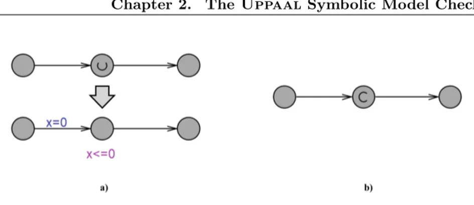
As shown in Fig. 2.1 a) an urgent location semantically corresponds to a location labelled with the invariant x  0. A committed location, depicted in figure 2.1 b), introduces a more restrictive constraint. In a network of TA, the state of the overall system is marked as committed if at least one of its TA is in a committed location. Since delay for this configuration is not allowed, the committed location must be left in the successor state, so only action transi-tions starting from a committed location are allowed. This means that although urgent and committed locations both guarantee a zero sojourn time, committed locations have priority over the urgent ones.

Chapter 2. The Uppaal Symbolic Model Checker

Figure 2.1: a) Urgent semantics b) Committed Location

2.1.2 Guarded commands

A transition, (referred as an edge in Uppaal), can be labelled with an action which, in general, consists of four optional fields, that are select, guard, synchro-nization and update, as follows:

[select][guard][synch i/o][update]

Each edge is enabled if the associated guard is true. If the guard is omitted, it evaluates to true. If an edge has no label, as shown in figure 2.2 a), the transition is said spontaneous.

The select component is useful for realizing a non-deterministic assignment, where the value is chosen in an interval of values. In addition, the select can be exploited for choosing a synchronization would multiple ones be ready.

The synchronization part of a command specifies one channel and an input/out-put operation on it. As indicated in Fig. 2.3, when a synchronization over a unicast channel is ready, with one sender and multiple receivers (or vice versa), one receiver is chosen non-deterministically by Uppaal. However, during veri-fication, all the possible choices are examined.

The update component is a comma-separated list of assignments, clock reset, or function calls. The operations in an update are executed from left to right. A guarded command constitutes the fundamental element for modelling con-current systems in Uppaal. It represents a basic atomic action. Semantics of Uppaal establishes that the update of the sender of a synchronization (ch!) is executed before that of the receiver(s) (ch?). This way the transmission of some arguments can be easily organized. In the case of a broadcast synchronization, the order of execution of the updates of the various engaged receivers, are car-ried out in the order in which the TA are listed in the system configuration statement which specifies the TA to be parallel composed.

Chapter 2. The Uppaal Symbolic Model Checker

2.1.3 Progress conditions

Besides the use of urgent and committed locations, the dwell-time in a normal location can be bounded through an invariant, which typically consists of a clock constraint (or conjunction of clock constraints). However, there are cir-cumstances where it cannot be possibly anticipated the amount of staying time in a location, but when a condition states the location should be abandoned, the exiting should be realized without delay. Toward this, the notion of an urgent channel (unicast or broadcast) can be exploited. If a synchronization is ready on an urgent channel, it must be taken immediately. In particular, the use of an urgent and broadcast channel can sometimes be preferable where, for instance, an output operation which is heard by no other process can be used for forcing the exit from a normal location. However, for implementation/efficiency rea-sons, Uppaal does not allow to check clocks on a guard in combination with a synchronization of an urgent channel. All of this, in turn, is related to the requirement that zones of a state graph be always convex.

Figure 2.3: Unicast synchonization: a) deterministic b) non-deterministic

2.1.4 Global time and clocks

Uppaal uses a continuous time model, in which the global time value is not directly accessible, but it can be checked through the use of clock variables. Clocks allow to measure relative time amounts, such as the elapsed time from a given global instant when the clock was last reset. The value of a clock varies in dense intervals. It can be reset and compared exclusively using natural constants. After being reset, all the clocks of a model automatically advance with the same rate (first derivative equals to 1).

The example in figure 2.4, taken from [27], shows typical clock behavior. The overall system is the composition of two automata, which model a user and a lamp respectively. The user can press a button to switch on a lamp. The first press puts the lamp in a moderate light. A subsequent press, which occurs within 5 time units from the previous one (two consecutive close presses) causes the lamp to bright. A next press will put off the lamp. From the low location, if 5 or more time units elapse, the lamp gets switched off. The behavior is regulated through setting and checking a clock variable y.

Chapter 2. The Uppaal Symbolic Model Checker

Figure 2.4: A simple lamp example taken from [27]

2.2 Query language

A network of TA can be inspected (i.e., tested) using the simulator component, by launching a single execution with a random choice of the next transition to be performed, or, it can be verified against some properties through the model checker engine, i.e. the verifyta kernel (see Fig. 2.5).

The properties to be verified are to be formally expressed using a subset of the Timed Computation Tree Logic (TCTL) [14]. Each query returns true when the property is satisfied, false otherwise. Like in TCTL, the query language consists of path formulae, that are in charge to infer properties over path or traces of the model, and state formulae, that describe what happens in individual states. Uppaal, though, does not allow nesting of path formulae [27]. A state formulae

Figure 2.5: Example of how in the Uppaal toolkit GUI is possible to select a sub-environment

is an expression that can be evaluated for a state, without considering the overall behaviour of the model. The syntax of state formulae is a superset of that of guards, which provides for the use of logical connectors (&&, and, ||,or, !, not, imply) and it includes:

• logical conditions on data or clock variables; • testing if an automaton is in a particular location; • or a logical combination of the conditions above.

A default property, which is not strictly a state formula, is expressed by the keyword deadlock, used for checking for the possible presence of deadlocked states.

Path formulae can be classified into three categories:

• reachability: which has the task of verifying if a certain state can be achieved;

• safety: who is responsible for ensuring that the system does not come into a dangerous state (such as deadlock);

Chapter 2. The Uppaal Symbolic Model Checker

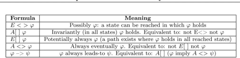
Formula Meaning

E < > ' Possibly ': a state can be reached in which ' holds A[ ] ' Invariantly (in all states) ' holds. Equivalent to: not E<> not ' E[ ] ' Potentially always ' (a path exists where ' holds in all reached states) A <> ' Always eventually '. Equivalent to: not E[ ] not '

'–> 'always leads-to . Equivalent to: A[ ] (' imply A <> ) Table 2.1: Path formulae supported in Uppaal

• (bounded) liveness: whose task is to test if the system evolves towards some state (possibly within a given finite time);

that can are always investigated in terms of reachability on the state-graph. Reachability properties can be used to validate a model, by checking the occur-rence of expected or unexpected behaviour. Given a state formula ', they are in charge to verify if ' can be satisfied by any reachable state (even after an infinite time), i.e., if there exists a path starting from the initial state, such that 'is eventually satisfied along that path. The path formula used to check these kinds of properties is in the form E ⇧ ', while in Uppaal it can be expressed using the syntax E<> '.

Safety properties are used to ensure that the system does not have unwanted behaviours. In Uppaal these properties are formulated positively, i.e., in terms of something good is invariantly true. Let ' be a state formula, it is possible to express by using:

• A⇤' that ' should be true in all reachable states;

• E⇤' that should exist a maximal path (that is an infinite path or where the last state has no outgoing transitions) such that ' is always true; In Uppaal these formulae can be written as A[ ] ' and E[ ] ' respectively. Live-ness properties aim to guarantee that the desired state will be finally reached in the system. In its simple form, liveness is expressed with the path formula A⇧', meaning that ' is eventually satisfied. The more useful form is the leads to property, written as ' which is read as whenever ' is satisfied, then inevitably will be satisfied. In Uppaal these properties are written as A<>' and ' - - > . Note that the liveness property cannot be verified from normal locations, where on the exit edges there are at the most normal channels, be-cause the process can stay there for an unbounded time.

Figure 2.6 and Table 2.1 summarizes the operational meaning of the basic queries.

When a property is not satisfied, Uppaal (if requested) can generate a counter-example, called diagnostic trace, automatically loaded in the simulator, which allows to see step-by-step the sequence of transitions that lead to the problem. A diagnostic trace can also be created when an existential query gets satisfied.

2.3 Advanced features

In latest versions of Uppaal, new features were introduced which enable the modelling of hybrid systems, that combine discrete and continuous behaviors.

Chapter 2. The Uppaal Symbolic Model Checker

Figure 2.6: Path formulae supported in Uppaal, taken from [27]

Figure 2.7: Example of over-approximation

Toward these clock variables are allowed to have different rates of advancement, regulated by putting into locations, as invariants, a first derivative of the clock different from the 1 default value. In addition, clocks are allowed to be stopped (stopwatches), thus retaining their values, and subsequently restarted from the value they were last stopped. These features are, for example, of interest when modelling preemptive real-time tasks [68, 88]. A preempted task, caused by the arrival of a greater priority one, has the need to frozen its clock which is measuring the execution time of the task body. All of this can be achieved by entering a location where the invariant states the first derivative of the clock variable is equals to zero. When the scheduler decides that a preempted task can again be released on the cpu, it is sufficient to force the exiting from the frozen clock location.

Unfortunately, the use of stopwatches does not come without problems. On the other hand, hybrid systems in most cases tend to be undecidable. It can be shown that a model with stopwatches generates not convex zones thus com-plicating the model checking (which sometimes cannot possibly terminate). In these cases, Uppaal resort to using the Over Approximation (OA) technique

Chapter 2. The Uppaal Symbolic Model Checker [31] which is not always capable of furnishing certain results. Under OA a not convex zone is enlarged so as to cover the original zone and become convex (see the example in Fig. 2.7 taken from [] for the general concept of how a not con-vex zone can be transformed into a concon-vex one). Obviously, an enlarged zone includes states which do not exist in the original model. Therefore, the issue of some queries can be inconclusive. In particular, properties which are invariably true (safety A[ ] queries) on the OA based model, are certainly true also on the original model. An existential property which is satisfied on the OA based model, can be true on states introduced by the OA which do not belong to the modelled system. As a consequence, the concept of a property which might be or not satisfied arises.

Chapter

3

Probabilistic and Statistical

Model Checking

Distributed probabilistic/stochastic timed systems represent a grand challenge for modelling and analysis. Symbolic model checkers like Uppaal can only evalu-ate some logical/temporal properties of these systems. In fact, when faced with a probabilistic and timed model, Uppaal ignores probabilistic aspects and turn probabilistic execution paths into non-deterministic paths. All of this is impor-tant but a full characterization of the behavior of these system models requires deriving a probability measure of event occurrences. On the other hand, exhaus-tive verification can incur into state explosion problems. Nowadays, Probabilistic and Statistic Model Checking represent two automated formal verification meth-ods, that given a stochastic model M and a logical property ', can perform two kind of analysis (possibly approximate) [153]:

• qualitative: is the probability for M to satisfy ' greater than or equal a certain threshold k (P (') k)?

• quantitative: what is the probability for M to satisfy ' (P=?('))?

Analysis can exploit numerical or statistical techniques. The numerical ap-proach checks the system using symbolic methods based on boolean formulas, or numerical methods [230]. Although accurate, this approach does not scale well and can be computationally expensive, being centred on the construction of a probabilistic timed system based on Markov chains and related timed vari-ants [204], it can also be affected by state-space explosions [164]. The statis-tical approach, instead, although potentially less accurate, does not suffer of state-explosions, because it relies on Monte Carlo simulations. It provides a quantitative measure (p-value) of confidence of its answer using first a sampling phase, in which the system is simulated for a finite number of runs, e.g., estab-lished by Wald’s hypotheses [255]. Then statistical inference is applied either according to the hypothesis testing phase, used to infer whether the samples provide statistical evidence for the satisfaction or violation of the specification [263], or with an estimation phase whose aim is to determine likely values of parameters, based on the assumption that the data are randomly drawn from

Chapter 3. Probabilistic and Statistical Model Checking a specified type of distribution [9]. Intuitively, since this technique rests on a proportion of the results extracted from the various runs (with the amount of required memory which is linear with the model size), to obtain more accurate results the number of samples needs to be increased, thus implying a longer computation time.

In this chapter, first concepts of Probabilistic Model Checking are discussed, then the operation of Statistical Model Checking (SMC) is reviewed. SMC is chosen in this work for quantitative evaluation of distributed probabilistic and timed systems.

3.1 Probabilistic Models

Probabilistic model checking is an extension of model checking, applied to sition systems augmented with information about the likelihood that each tran-sition will occur [141]. The behavior of a model with a set of states S is not specified by a transition relation on S, but through a transition function. In order to carry out their operations, probabilistic model checkers require as input:

• a probabilistic model of the system;

• a temporal logic specification language, used to express qualitative and quantitative properties under investigation.

Table 3.1 summarizes some probabilistic models often used to build a formal description of a system with stochastic behavior, whose concepts are then briefly summarized.

Time Non Deterministic Probabilistic Models Discrete no Discrete-time Markov Chains (DTMCs)

yes Markov Decision Processes (MDPs)_{Probabilistic Automata (PAs)} Continuous no Continuous-time Markov Chains (CTMCs)

yes _{Priced Probabilistic Timed Automata (PPTAs)}Probabilistic Timed Automata (PTAs) Table 3.1: Types of probabilistic models

3.1.1 Discrete-Time Markov Chains (DTMC)

Discrete-Time Markov Chains (DTMCs) are fully probabilistic transition sys-tems, in which the successor state of a process does not depend on the satis-faction of a guard, but it is chosen probabilistically within a set of admissible states. In a DTMC, transitions can occur at discrete time-step n = 0, 1, 2, . . . , so if the system enters a state s at time n, it stays there for one time unit and then moves to s0 _{at time n + 1 [204].}

DMTCs are well suited for modelling, for example, simple random algorithms or synchronous probabilistic systems where components evolve in lock-step. Formally, a DTMC is a tuple M = (S, s0, M, L)where:

Chapter 3. Probabilistic and Statistical Model Checking • s02 S is the initial state;

• M : S⇥S ! [0, 1] is a transition probability function, that assigns probabil-ities to successor states, with the requirement: s 2 S,Ps0_2SM (s, s0) = 1; • L : S ! 2AP _{is a labelling function, which assigns to each state s 2 S a}

set L(s) of atomic propositions a 2 AP ;

A DTMC satisfies the Markovian property (absence of memory): the probabilis-tic description of the system at time n + 1, only depends on the current state at time n, and not on the previous history; this implies that the sojourn time in a state is distributed according to a geometric distribution.

Graphically, a DMTC is represented:

• by an direct graph, in which states, labelled with atomic propositions, indi-cate a specific execution circumstance of the system, and edges, weighted with probability values, represent the eligible transitions with non-zero probabilities;

• by a transition probability matrix, in which rows and columns are labelled with states and the element at (i, j) represents the probabilistic weight associated to the transition from the status si to sj.

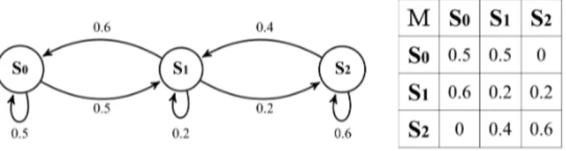
Figure 3.1: Example of a Discrete Time Markov Chain and its transition probability matrix

Figure 3.1 shows an example of the two ways of representing the so called ho-mogeneous DMTC, in which the probability values associated with transitions are costant and do not depend on the time-step n.

A run or path ⇡ in a DMTC M is defined as a sequence of states and transi-tions s0 p0 ! s1 p1 ! . . . pi! s1 i pi ! . . . with i 2 N, si 2 S, and pi 2 R(0,1]

such that pi > 0 ^ pi = M (si, si+1) for all i 0. It is indicated with

⇡:n _{= s}

0, s1, . . . , sn 1, sn [212]. Due to the Markovian property, transitions

between states are selected independently from each other, and the probability of reaching a given state, following a path ⇡, is given by:

PM(⇡) = n 1_Y i=0

M (si, si+ 1) si, si+12 ⇡

Considering the DMTC M in figure 3.1 and the path ⇡ = s0, s0, s1, s0, s1, s2,

the probability of ⇡ is PM(⇡) = 0.5· 0.5 · 0.6 · 0.5 · 0.2 = 0.015.

In order to carry out performance analysis on discrete-time and stochastic model, classical Computation Tree Logic (CTL), introduced by [82], has been

Chapter 3. Probabilistic and Statistical Model Checking enriched to handle and formulate probabilistic queries. The Probabilistic Com-putation Tree Logic (PCTL) proposed by [116], provides the following syntax for query formulation [166]:

::= true | a | 1 ^ 2 | ¬ | P⇠p[ ]

::= X _| 1Uk 2 | 1U 2 | F | G

where a is an arbitrary atomic proposition, p 2 [0, 1] a path probability value, ⇠2 {<, , , >} one of the possible inequality operators, and k 2 N an arbi-trary natural number. The formula is used to verify properties on a specific state of the model, whereas formula is used to investigate the satisfaction of constraints over a path.

Compared to the basic CTL version, two new expressions are added:

• the formula P⇠p[ ], that is true in a state s 2 S when the probability that

holds on paths starting from s exceeds a certain threshold (⇠ p);

• the bounded until operator 1Uk 2, that is true for a path ⇡ = s0, s1, . . . , sk, . . .

whenever there is a state sn+1with n + 1  k where 2holds, and for all

states up to including sn, 1 holds (see equation 3.1) [9].

s0 s1 . . . sn sn+1 . . .

1 1 . . . 1 2 . . . (3.1)

3.1.2 Markov Decision Processes (MDPs)

Some aspects of a system which may not be modelled probabilistically, include: • concurrency in the scheduling of parallel components;

• unknown environments;

• underspecification, i.e., unknown model parameters.

To model these aspects, the concept of Labelled Transition System (LTS) where the choice of the next state is nondeterministic, can be combined with that of DTMC where the next state is chosen probabilistically.

A Markov Decision Process (MDP) is a discrete-time state-transition system with both nondeterministic and probabilistic behavior. As in a DTMC, tran-sitions between states occur in discrete time-steps and a discrete set of states represent possible configurations of the modelled system. Formally, it can be described as a tuple M = (S, so,A, T, R(s)) where:

• S is a finite set of states; • soare the initial states;

• A is a set of actions used to control the system state. The set of ations that can be applied in s 2 S are labelled as A(s), where A(s) ✓ A; • T is the transition probability function T : S ⇥ A ⇥ S ! [0, 1] that

de-scribes the probability of reaching state s0 _{after doing an action a in}

state s: T (s, a, s0_{) = P r(s}0

t+1|st, at). For all states s and actions a,

P

s0_2ST (s, a, s0) = 1, i.e. T defines a probability distribution over possible next states.