Are Regional Inequalities Decreasing with Public Investment? Evidence from Mexico

Testo completo

(1)Robert Schuman Centre for Advanced Studies. Are Regional Inequalities Decreasing with Public Investment? Evidence from Mexico. Eduardo Rodríguez-Oreggia and Joan Costa-i-Font. RSC No. 2002/19. EUI WORKING PAPERS. EUROPEAN UNIVERSITY INSTITUTE RSC 2002/19 © 2002 Eduardo Rodríguez-Oreggia and Joan Costa-i-Font.

(2) All rights reserved. No part of this paper may be reproduced in any form without permission of the authors.. © 2002 Eduardo Rodríguez-Oreggia and Joan Costa-i-Font Printed in Italy in March 2002 European University Institute Badia Fiesolana I – 50016 San Domenico (FI) Italy. RSC 2002/19 © 2002 Eduardo Rodríguez-Oreggia and Joan Costa-i-Font.

(3) ABSTRACT Traditional economic theory predicted in the past that public investment may reduce regional inequalities improving growth in poorer areas. However, recent theoretical and empirical contributions suggest an opposite causality, especially when countries are involved in regional and trade integration arrangements. Under the former context, public investment may be widening the gap between regions. This paper empirically investigates how the assessment of public investment at the central influences regional inequalities. We use data on Mexican regions we test the extent to which public investment is associated with regional inequalities. Empirical methods used are standard regression and quantile regression models allowing the measurement of regional income at different quatiles of the income distribution. Findings suggest that public investment had a negative influence on reducing regional inequalities and inequality reduction was more prominent between the set of richest regions. Keywords: regional inequalities, public investment, and quantile regression..

(4) INTRODUCTION Regional policies in occidental countries have been largely influenced by a tendency to invest in infrastructure under the logic that public investment may have a positive impact on regional productivity and thus may lead to reduce regional inequalities. Accordingly, public investment is conceived as a regional policy instrument to influence both economic growth (Aschauer,1989; Costa et al, 1987; Munnell, 1990a, 1990b; Gramlich, 1994; De la Fuente,1996a) and the distribution of economic activity (De la Fuente,1996b; Cuadrado-Roura, 1988). However, under an economic integration setting, public investment may lead to unequal gains to regions. In particular, benefits may be larger for border regions when a free trade agreement is set up, and those regions with previous advantages from economic agglomeration or natural resource endowments may benefit the most from integration processes. In Mexico these would refer to the northern regions, the oil producing regions, and surrounding areas of Mexico City. Consequently, public policy in Mexico may show two main alternatives. First, investing in poor regions may envisage a public policy to counteract differentials in economic activity derived from differentials trade intensities, encouraging a process of convergence in which poor regions are intended to grow more than richer ones or alternatively, may lead to investing in those regions that can benefit the most from trade with, leading to a higher country growth rate although increasing regional inequalities. Evidence form the EU shows that regional disparities do not diminish under trade integration settings as regions with the lowest output levels have not grown faster that regions with higher levels of output (Cuadrado-Roura,1994). There are strong reasons to argue that public investment may increase regional inequalities. The most comprehensive research in this regard is Martin and Rogers (1995) and Martin (1999) provide a comprehensive argument. Martin sets out a model that shows how improvements in infrastructures, by reducing transaction costs inside the poorest region, provide incentives to firms not to localise in poor areas, which in itself may increase the regional income gap. The aim of this paper is to examine the impact of the current allocation of central public investment in reducing regional inequalities. Previous empirical literature is not conclusive in this matter. Moreover, to our knowledge, this is the first empirical research focused on measuring the impact of public investment on regional application in Mexico differentiating according to the income position. A key aspect of this paper is the original empirical method used: the quantile regression models. The application to Mexico is especially relevant as has a federal structure with well known large regional differences. Further,.

(5) although decisions for the use of public investment are taken locally, the amounts are centrally allocated and thus a regional analysis is especially interesting. We use quantile regressions that allow us to investigate the contribution of public investment at different points within the regional income distribution function. This is a relative innovation in the empirical techniques used until now. A database collected from public sources was used to describe the implication of our results for the design of public policy aiming to reduce the regional income gap. The structure of the paper is as follows. Section two present a context for the Mexican situation. Section three deals with the theoretical framework and previous literature on the issue. Section four describes the model and data. Section five the results. Finally, some concluding remarks are outlined. THE MEXICAN MACRO ENVIRONMENT AND RECENT REFORMS The year 1970 ca be seen as the end of the "stabilising development period" that lasted from the 1950s to the ends of the 1960s. In this period the Mexican economy grew at rates of 10% what leads to an opening period of populism in the Mexican government. During the 1970s and beginning of the 1980s the Mexican economy grew at a rate of 6.7%. Motors of growth during this period can be partially explained by public investment. Public investment was mainly financed through public deficits and debt. A good part of this can be attributed to the oil boom, when new oil fields were found and the prices were high in the international market, creating good expectations for the next years. Long term expectations of high oil prices were the genesis of a considerable external debt to finance public investment. At the beginning of the 1980s oil prices decreased leading to a debt crisis in 1982 and 1985 and international finance organisations closed credit lines to Mexico. The reschedule of the debt led to an economic adjustment to set conditions for a new period of economic growth and financial solvency. The economic adjustment implemented during the period 1983-1988 was directed towards two main objectives (CARDENAS, 1996). The first was the reduction in the size of the public sector, through the sell of public enterprises, deregulation of markets and cuts in public budgets. The second was the trade liberalisation to open the Mexican economy, decreasing the number of tariff and trade barriers, and specially to become a member of the GATT. A main characteristic of the structural adjustment was the necessity of the government to extract from the society all the resources to transfer as debt payments. These resources were extracted from real wages, using the inflationary tax, leading of course to a drop in real wages during the whole period. 5.

(6) With the government initiated in 1988 a new plan launched a far reaching process of deregulation of economic sectors, privatisation of public enterprises and reductions in budget expenditures leading to a drop in inflation and reductions in the public debt and budget deficit. There was also a new confidence of the international investment due to the restructuring of international debt through the Plan Brady, and the signing of the North America Free Trade Agreement with Canada and the US. Short-term financial markets made vulnerable external fluctuations. In addition, the decision to continue fighting against inflation with a highly undervalued exchange rate, plus the political instability generated in 1994 led to a interruption of foreign capital flows, halting the financial system and guiding to a devaluation of the peso and the decision to let it to float. International investors withdrew their funds not only from Mexico but also from all Latin America stocks markets, originating the "Tequila effect". The new government authorities (1994-2000) implemented a new plan with tight fiscal settings, control of inflation, anticipation of debt maturities that immediately restored credibility of international investors in the government policy. If this crisis led to a fall of 6.2% of the GDP in 1995, the new adjustment plan brought an increase of 5.1% of GDP in 1996 (respect to 1995), led essentially by a surge in Mexican exports and investment, mainly in the export oriented sectors (OECD, 1997). Table 1 Coefficient of Variation of per capita GDP Year 1970 1980 1985 1988 1993 1996. All Regions* 0.43 0.38 0.34 0.43 0.47 0.48. Centre. North. South*. 0.49 0.49 0.44 0.52 0.62 0.63. 0.20 0.20 0.18 0.18 0.17 0.15. 0.41 0.42 0.31 0.56 0.70 0.64. *Excluding Campeche and Tabasco. All these macroeconomic issues have implied an effect on regional disparities. To assess to what extent disparities among regions in Mexico have grown we calculated the coefficient of variation of per capita GDP for different years and grouping by geographical zones, as is depicted in Table 1. These results show 6.

(7) that the disparities of per capita GDP reduced during the period from 1970 to 1985. As we have remarked, 1985 is the year in which Mexico started its trade opening with other countries. The big leap in the income dispersion between states occurred in the period 1985-1988, and since then has remained almost constant. Disparities in the second half of the 1990s are higher than levels in 1970. Northern states have the lower and decreasing disparities, while states in the South show higher disparities of income. In this context of macroeconomic imbalances and increasing regional disparities, the allocation of public investment has been supposedly to increase its focus and efficient allocation at the regional level, in opposition to previous period with discretional allocation of public investment (Bazdresch and Levy, 1991). A point of reference of planning in this issue is the National Development Plan, which is elaborated as a guideline for every government for 6 years. The National Development Plan 1989-1994 (Poder Ejecutivo Federal, 1989) aims to influence the economic growth process through the direction of public investment. It declares that one of the main purposes of this kind of policy is to move forward decentralisation and co-ordination in budget assignment, and together with local governments participation achieve financial autonomy, while at the same time they are increasing their sharing in resources and its making. This plan emphasises the importance of infrastructure in communication and transport for sustained growth, suggesting that private investment should complement the state's activity. It also remarks that one of the main objectives is to develop and improve this kind of infrastructure in order to support growth policy as well as regional development and integration. The plan sets as priority to invest in infrastructure facilitating the communication and transport services supply for low-income areas. The National Development Plan for the period 1995-2000 (Poder Ejecutivo Federal, 1995) sets poverty eradication as the main concern when deciding where to allocate public investment, focusing on areas with great economic and social disadvantages. It has as purpose to give shape to a new social, integral and decentralised policy, concentrating efficiently and effectively on less developed groups and regions. In the regional development section, this plan states that development policy will look to close gaps between regions and specific areas on the country through the channelling of more resources and the creation of sufficient conditions for productive investment in zones with notable disadvantages. The plan remarks as a key factor investment in infrastructure, which in a parallel. 7.

(8) direction with local development capacities could link less developed regions with the more developed ones. In tackling disparities between regions, the plan sets that definition of regions and co-ordination procedures will be decided on priorities established by local governments, and also in the context of the social and productive integration incorporating the lagged groups to development. A crucial point for regional development in the plan is the allocation of public and private investment. In so doing, economic diversification will take place, fostering more links between rural and urban economies, and strengthening economic and administrative capacity in local governments. The purpose of the paper is to analyse, in this context of growing inequalities among regions in Mexico, the role of public investment in closing the differences in per capita GDP among them as mentioned in the National Development Plans. More specifically, we seek to measure the extent of the impact of public investment in regional disparities according to the respective position of regions on the income distribution scale. In order to analyse this, we first will review the theoretical effects of public investment on disparities in such a way that we can outline a model for the analysis in the following sections. THE ROLE OF PUBLIC INVESTMENT ON DISPARITIES In reviewing the role of public investment on growth and disparities it is necessary to consider two issues: how public investment is allocated, and to what extent there is an impact of this allocation on regional disparities. Public investment1 allocation and growth In middle income countries there is an observed pattern of scattering funds among a large number of small projects dispersed through the nation (Hirschman, 1958). One reason for spatial scattering of investment is the political support for the government in all regions of the country. Then, there is an incentive to scatter the investment extensively. Another incentive is the belief that economic progress is a force affecting equally all regions. In addition, governments are unprepared and unwilling to take decisions about spatial priorities and sequences for investment. Nevertheless, Hirschman's argument of leaves to the planners the criteria to switch the direction of public investment, which could be manipulated in electoral terms.. 8.

(9) The time for switching the allocation of investment was modelled by RAHMAN (1963). The central assumption of his model is that central planning investment is intended to maximise the national rate of growth, also that there are regional demands for an economic process without wide disparities in regional living standards. These findings seem to be reinforced by Intriligator (1964), who found that the optimal allocation of regional investment is very sensitive to the objectives settled by the planner. His model suggests that the maximisation of terminal income leads to switching investment from regions with high growth to regions with high output-capital ratio. It also implies that the maximisation of per capita consumption during the planned period leads to a switching from high output-capital ration regions to high growth regions. Beyond these findings, Okuno and Yagi (1990) examine those aspects of public investment that tend to balance interregional income equality and efficiency of the economy as a whole. Including private investment in the model, they found that the public investment switch from rural to urban is an optimal policy, while ignoring private investment the switching is not optimal. They found regional income inequality affected by public investment, showing that this allocation aimed at reducing regional output inequality does not always produce the desired effect. Martin and Rogers (1995) and Martin (1999) suggest that public infrastructure may play a role in attracting industries from other regions. They state that there is an increase in local welfare because of the relocation of industry originated in the enhancement of public infrastructure, while there is a decrease in foreign welfare. Furthermore, given the consumption of real resources to improve public infrastructure, the characteristic of a non cooperative equilibrium may be characterised by a sub-optimally high level of domestic infrastructure. Although the issues related to the regional allocation of public investment began with Hirschman (1958), its role on growth models was taken into account with the Aschauer (1989) and Munnell (1990a, 1990b) works. Public investment is intended to generate benefits through economic growth, mitigation of poverty and other issues, given that it involves goods and activities increasing the productivity of private factors. However, this process has been subject to criticism as results are mixed in the empirical evidence. There are more problems related to the common trends in public investment (Munnell, 1992), to methodological limitations when evaluating and understanding the returns to investment (Morrison and Schwartz, 1996; Gramlich, 1994). Despite this, conclusions in most cases point towards an important role of public investment in shaping growth.. 9.

(10) Growth and disparities Following the work of Barro and Sala-I-Martin (1991, 1992) on the pattern of growth at regional levels there have been a number of works interested in investigating the common speed at which economies converge to their own steady state. These ideas are supported by neo-classical growth theory, supposing a downward sloping saving curve, meaning diminishing returns to capital. The implication behind diminishing returns to capital in neo-classical models is that each addition to capital will generate a huge addition in output when the capital is small, and small addition when the capital is large. Consequently, if there is only one difference across economies, the initial capital stock, poor regions (with small capital stock) will grow faster than rich regions (with large capital stock), creating a convergence effect. What is obtained from the analysis is the b convergence coefficient. This coefficient quantifies the mobility of income within the same distribution, and there is b convergence if poor regions are growing more than rich regions. When including some variables in the analysis it turns to be a conditional beta convergence. However, this approach has been consistently criticised. In particular, one point is labelled against it, which is that a cross section regression to explain time averaged growth rates is inappropriate, therefore, the signs of the initial levels coefficients do not reflect the process of divergence or convergence, and also produces the apparent 2% rate of convergence (Quah, 1993b) through what is called the Galton’s fallacy. The convergence approach also fails to provide information about permanent movements in income through time trends (Quah, 1993a). In this sense, Markov chains are proposed in the regional context to measure the connections between aggregate fluctuations and regional dynamics. This process allows the analysis of intra distribution movements of income, and the income transformation from one year to another between groups. Nevertheless alternative statistical models can differ strikingly, although is not easy to differentiate, with typical data available, between these models (Fingleton, 1997). Moreover this method does not allow us to measure to what extent other policy variables are affecting growth among groups of incomes. Other alternatives have been sought. De la Fuente (1996c) uses a conditioned regional convergence model with technological diffusion and capital accumulation, finding an important contribution to regional disparities, although there is a large component unexplained in the long term. CuadradoRoura et al. (1998, 2000), using panel data, add to the analyses of convergence a 10.

(11) set of variables including the regional productive structure, and open the model to more variables such as infrastructure, education, regional dummies, etc., calling these effects "fixed factors". Moreover, it is not possible to analyse to what extent these variables are impacting growth according to regions positioned in different levels of the income distribution. However, even though the literature used refers to income differences, most of them use growth. To what extent can we imply that growth reduces disparities? As Robinson (1972, pp 7) states: " a growth in wealth is not at all the same thing as reducing poverty". Evidence that growth does not necessarily reduce inequalities can be found in Cuadrado-Roura (1994). Furthermore, Chatterji (1992), using a set of countries for analysis, found a group of countries converging towards the US per capita income, while another group were converging towards a thirtieth of the US per capita income. Then, the division between poor and rich could be deepening, while the aggregate measure for convergence can show a process for convergence. All these problems suggest that additional ways of testing growth and disparities should be carried out (Cheshire and Carbonaro, 1995). In this paper, we go further and identify how the process of regional convergence is evolving according to the position of the regions in the income distribution. However, as has been remarked the main aim of the paper is to identify the role of public investment in increasing or reducing regional disparities. In doing so, we will analyse the impact of public investment on GDP per capita by quantiles of income and establishing two sets of analysis. The first based on growth, and the second based on regional inequalities. THE MODEL AND EMPIRICAL APPLICATION The empirical Model The empirical strategy used in this study is based on first analysing the role of public investment (PUBINV) in regional inequalities of income (I) and growth (Y). To do so we have included a set of control variables. First, a variable of initial per capita GDP (INGDP) in order to capture the effect of previous regional differences as has been noted in the theoretical section. The variable employed is the logarithm of 1993 GDP per capita. Second, we use a set of dummy variable to isolate the effect of being an oil producer (OIL), a region in the (NORTH) or in the (CENTRE) of the country2. The reference then is the SOUTH, the less developed area in the country. To some extent, this allows us to compare with the "fixed effects" introduced by Cuadrado-Roura et al. (1998) through dummies for specific regions. Finally, we introduce the variables for public investment (PUBINV). Nevertheless, in order to avoid to some extent the 11.

(12) problem of possible simultaneous bias between regional GDP per capita and public investment, we introduce lags in the variable of public investment. The index for regional inequality in per capita GDP is defined as: I it = y DFt - y it. (1). Where i is the state and t the period of time, yit is the log of per capita GDP for each state in the period t, yDF is the log of per capita GDP corresponding to Mexico City, the region with the highest per capita GDP in the sample during the period to analyse. This index was used by Chatterji (1992) to determine the pattern of income gap in a sample of countries, and the gap is measured strictly with positive numbers for every region (except Mexico City for which the gap is zero). The index was first proposed by Abramovitz (1986) as an indicator for the catch-up of any region or country. a) The OLS model The models to estimate are the following: Yit = a + b1 INGDPit + b 2 OIL + b 3 NORTH + b 4 CENTRE + b 5 PUBINVit + b 6 PUBINVit -1 + b 7 PUBINVit - 2 + m it. (2) and I it = a + b 1 INGDPit + b 2 OIL + b 3 NORTH + b 4 CENTRE + b 5 PUBINVit + b 6 PUBINVit -1 + b 7 PUBINVit - 2 + m it. (3) Where m denotes the error term. The coefficients of public investment will be informative of the relationship between public investment and regional inequalities. In the inequality equation a positive sign is expected according to Martin (1999), a negative sign would indicate a redistributive process, while in the growth equation we should expect a positive sign according to the theory. Initial per capita GDP is to show a negative sign in the growth equation if there is a process of convergence, then in the inequality equation we should expect a positive sign if the catch–up assumption in growth models applies. Finally, dummy variables may show ambiguous signs.. 12.

(13) These results, although informative, provide little information on the effects of public investment and other related determinants on income inequality as they may hide differential effects within groups of regions. An alternative way of looking at this issue is using quantile regression analysis, which enables us to distinguish between those regions situated in the extremes of the inequality and growth distribution such as those situated in the median distribution. a) The quantile model In ordinary regression models, we cannot distinguish if growth and inequalities are appearing in the whole spectrum of distribution or are concentrated in some quantiles of the distribution. In order to elucidate this issue, we estimate a quantile regression model. Quantile regression models are based on the work of Koenker and Basset (1978), and have been extensively used in labour economics to study wage inequalities (Garcia et al, 1999). We use this method to analyse changes in regional inequalities at different points of the income distribution. Let ( I it , PUBINVit ) be a sample of two main explanatory variables for a given period. The relation between these two variables may be formulated as: I it = b o PUBINVit + m 0i. (4) Then the quantile regression can be expressed as: Quantq ( I it / PUBINVit ) = b 0 PUBINVq. (4) Where the Quant denotes the conditional quantile (q ) of I it and the regressor vector PUBINVit assuming that Quantq (U oi / PUBINVit ) = 0 , where Uqi is the error term. The estimation results Quantˆ( I it / PUBINVit ) = bˆq PUBINV indicate how inequality will vary as q increases in the distribution. Therefore the quantile coefficients informs us about the marginal change in the conditional quantile due to a marginal change in PUBINV. The data The data used for the Mexican regions was collected from public sources to form a panel of data for the period 1993-1998, which coincides with a great trade openness with other countries. We are using the state level unit as data is available for longer periods and gathered more consistent and frequently. Data for GDP was gathered from the Instituto Nacional de Estadistica, Geografia e Informatica (INEGI) from 1993 to 1996a period in which the country has been immersed in a deep process of trade liberalisation. To calculate per capita GDP 13.

(14) we are using population data from the Population Census by INEGI and figures from the Statistical Annexes of the Presidential Address to the Nation many years. Data on public investment was collected from 1993 to 1998 from the same Statistical Annexes. The dataset was used to calculate the per capita public investment channelled to the region i, as a share of the national average of per capita public investment. We are considering for Mexico as public investment concepts such as education, health, housing, labour, regional and urban development, ecology, social supply, the Solidarity programme and transport and communication concepts, that is we include the social and economic concepts of public investment. As we can expect a differentiated effect of public investment according to the region inequality, we determine some dummy variables. The dummy variable for oil states comprises Campeche and Tabasco states, in which there was a high proportion of public resources channelled into exploration and exploitation of oil fields. There are also dummy variables for the Northern states, including states with borders to the US, and a dummy for Centre states comprising all the states around Mexico City (see note 2). RESULTS Using panel data for the Mexican regions Table 2 shows results for the growth equation, Table 3 depicts results for inequalities. Table 4 shows the coefficients for variance inflation factors (VIF) to test for multicollinearity, and the low factor values suggest that there are no problems with multicollinearity. The first column in Table 2 and 3 show results for OLS regression, while the other columns show outcomes for the quantile regression. The quantiles regressions for growth comprise regions with more growth in the higher quantile (0.75), and in the lower quantile (0.25) regions with low growth. In the inequality Table, the higher quantile (0.75) comprises regions more unequal, that is, those with a greater distance from the leader, while the lower quantile (0.25) includes regions with lower indices of inequality, that is, the richest regions. Tests for heteroscedasticity were made through the Cook-Weisberg test and when necessary the standard errors were corrected with the White-Hubert-Sandwich method. In the OLS results in Table 2 the initial GDP per capita (INGDP) has a significant and positive coefficient, suggesting a divergent process rather than convergence, although at a very slow rate. This finding is consistent with the evidence on convergence and divergence among Mexican regions found by Juan-Ramon and Rivera-Batiz (1996), who found a process of divergence 14.

(15) occurring since the end of the 1980s. If we look at the quantile regressions, the process of divergence is repeated in the lowest growth regions, while in the highest the coefficient is no significant. Thus, we cannot find formation of convergence clubs according to income distribution group of regions. Table 2 Growth in per capita GDP in the Mexican regions, 1993-1998 Variable PUBINV PUBINV(1) PUBINV(2) INGDP OIL NORTH CENTRE INTERCEPT R2. +. OLS 0.1696* (0.0407) 0.0918* (0.0296) 0.0356 (0.0305) 0.0042* (0.0011) -0.0100 (0.0062) 0.009* (0.0035) 0.0067 (0.0043) -0.003 (0.0025) 0.2554. Quantiles 0.25 0.5 0.1523* 0.1264* (0.0663) (0.0172) 0.0540 0.1011* (0.0479) (0.0178) -0.0173 0.0551* (0.0481) (0.0146) 0.0062* 0.0021* (0.0031) (0.0009) -0.0034 -0.0181* (0.0127) (0.0039) 0.0146 0.0010 (0.0085) (0.0025) 0.0112 0.0055* (0.0091) (0.0027) -0.0189* 0.0031* (0.0045) (0.0013) 0.1828 0.1294. 0.75 0.0604* (0.0255) 0.0882* (0.0261) 0.0667* (0.0241) 0.0020 (0.0013) -0.0202* (0.0057) -0.0021 (0.0037) 0.0021 (0.0042) 0.0146 (0.0020) 0.1196. Standard errors in parentheses. + Standard errors corrected for heteroscedasticity. ** Significant at a 5%. *Significant at 1% The effect of public investment is positive and significant in the OLS growth regression in Table 2, finding a positive and significant effect also for the first lag of public investment, but none significant for the second lag. The effect of the public investment for the year is significant in the quantiles, being higher for the lower growth regions. The first and second lags become relevant for the higher quantiles. The dummy variables are relevant only in the case of the oil producers in the higher quantile, although with a negative sign, more likely to occur due to the fall of impact of oil on the economy in the last years originated in the increase of the importance of other non-oil activities. The fact that public investment is impacting positively on growth is an interesting finding given that 15.

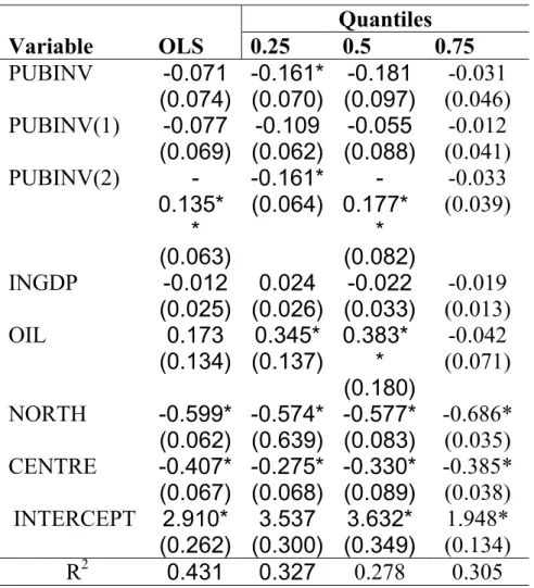
(16) as consequence of the recursive economic crises, public investment was cut in order to clear public finances (CARDENAS, 1996). Nevertheless, there is greater impact on the higher growth quantiles. To what extent does this imply there is an effect of public investment in closing differences among regions? This is what we analyse next with the inequality as dependent variable. Table 3 depicts results for the same regression but changing the dependent variable to inequality measured as in Equation (1). In this set of regressions it is important to note that the lower quantile comprises the richest states, as inequality is the distance to the leader in GDP per capita at the national level, while the highest quantiles include the states with higher distance to the leader, the poor states. This variable cannot only be read as inequality but it would also help to know the impact of the catching-up (Abramovitz, 1986) of the regions according to their distance from the leader and measuring the impact of public investment. Table 3 Inequality in the Mexican regions, 1993-1998 Variable PUBINV PUBINV(1) PUBINV(2). INGDP OIL. OLS -0.071 (0.074) -0.077 (0.069) 0.135* * (0.063) -0.012 (0.025) 0.173 (0.134). 0.25 -0.161* (0.070) -0.109 (0.062) -0.161* (0.064) 0.024 (0.026) 0.345* (0.137). NORTH. Quantiles 0.5 0.75 -0.031 -0.181 (0.097) (0.046) -0.012 -0.055 (0.088) (0.041) -0.033 (0.039) 0.177* * (0.082) -0.019 -0.022 (0.033) (0.013) -0.042 0.383* (0.071) * (0.180) -0.577* -0.686* (0.083) (0.035) -0.330* -0.385* (0.089) (0.038) 3.632* 1.948* (0.349) (0.134) 0.278 0.305. -0.599* -0.574* (0.062) (0.639) CENTRE -0.407* -0.275* (0.067) (0.068) INTERCEPT 2.910* 3.537 (0.262) (0.300) 2 R 0.431 0.327 Standard errors in parentheses ** Significant at a 5%. *Significant at 1% 16.

(17) The first column in Table 3 depicts results for the OLS regression. Although the initial per capita GDP is negative, there is no significant difference from zero. Public investment exerts a negative effect, suggesting that it has a redistributive component, although only the second lag is significant. Location around the leader and also locations next to the US market help to close differences. Now, focusing in the quantiles of inequality the initial per capita GDP is relevant although negative only for the higher quantiles, that is for the poor regions. This means that inside groups of poor regions, the ones with higher initial advantages are catching up faster than those with lower per capita GDP in the same group. In the lower quantile there is no evidence of any effect given that it is no different from zero. The effect of the public investment variables is relevant and negative only in the lower quantile of the inequality distribution, while the second lag is only relevant for the medium quantile. The variables are negative although not significant for the higher quantile of inequality. This suggests that public investment among the Mexican regions is playing a role of redistribution only among the richest regions, helping them to catch-up with the leader, while the effect is null in the needed regions. This is an interesting finding given that in the last decade public investment has been supposed to be more efficiently allocated compared to former periods (specifically 1970s and beginning of 1980s), when was allocated with no economic sense (Bazdresch and Levy, 1991). This finding is also opposed to the objectives of the National Development Plans of using public investment to reduce differences among regions. If the central government want to integrate lagged regions to development, as mentioned in the National development Plan, it need to readdress in a effective manner its policy for allocation of investment among regions, establishing more clear mechanism of allocation and redistribution. We must also note that dummy variables for distance are becoming relevant in all the quantiles and with high coefficients, suggesting that location around the leader (Mexico City) and to the US market helps to catch-up and close difference among the groups of regions. The oil producer states, although still rich are exerting a positive impact on inequality, suggesting the inverse process of catching-up, probably for the same reasons argued in the growth regressions. Finally, Table 4 shows the Variance Inflation factor (VIF) to the regressions in Table 2 and 3.. 17.

(18) Table 4 Variance Inflation Factor (VIF) for regressions in Tables 1 and 2 Variable PUBINV PUBINV(1) PUBINV(2) INGDP OIL NORTH CENTRE Mean. VIF 5.50 5.05 4.25 1.89 1.07 1.07 1.04 2.84. The findings can be interpreted under the ideas of Hirschman (1958), who stated that regional allocation of public investment is the most evident method through which policy influence rates of growth of different parts of a country. He distinguishes three patterns of allocation: concentration in more developed regions, concentration on potential growing areas, and promotion of backward regions. In consequence, disparities increase in the first phase, and decrease in the second. Examining the evidence, it appears that public investment has been allocated according to the first phase of Hirschman. Martin (1999) proposes that investment should be allocated in regions where transaction costs can be reduced due to concentration of industry. Investment in poor regions will lead then to increase in prices because of dispersion of industry as a decrease in welfare. In a future, the decrease in prices due to concentration will lead to a higher welfare and benefits for poor regions. This idea reinforces the first stage of Hirschman, although there is no switching to other regions. And also in this case, the findings in this work seems to confirm that allocation of public investment is done in more concentrated and rich regions, although to what extent this is increasing the welfare of other regions through price reduction is beyond the scope of this paper. The introduction of the quantile regression in the analysis of disparities has shown interesting insights, however more work has to be done in order to elucidate the effect and direction that disparities are taking place especially to elucidate the time for switching allocation of investment in specific regions.. 18.

(19) CONCLUSIONS Although some theoretical work has been undertaken to examine forms and times of investment allocation between regions, there is no clear-cut method developed yet. This paper has sought to analyse the influence of public investment in regional income disparities. The quantile regression technique used in this paper permits us to go further than a simple decomposition of income inequality in within or between groups. The main advance employing this technique is that we can isolate the impact of public investment on different sets of regions according to the position in the income and inequality distribution. Using data for the Mexican regions and looking to the determinants of regional growth we find that a process of divergence occurs among the lower groups of regions, while public investment has a clearly positive impact on growth in all the groups of regions. In the analysis of inequality we find that public investment has smoothed regional inequalities among regions within the richest group. Dummy variables for regions located around the leader and next to the US border show a positive and higher effect of catching-up. The strategy of the allocation of public investment may have followed a set of phases, which explains differences between the north and the south of the country, such as between oil producers or not. However, public investment is strongly associated with a reduction of regional inequality within the richest group of regions. The explanation for this phenomenon can be best understood under the Hirschman (1958) and Martin (1999) framework. This would predict that public investment should increase inequality especially within the regions located in the lowest quantile of the inequality distribution. As empirical results show, public investment has no relevant effects on those regions that are located in the top quantile of the inequality distribution. However, more empirical analysis should be undertaken to provide some insights to this issue. Eduardo Rodriguez-Oreggia London School of Economics Email: e.oreggia@lse.ac.uk Joan Costa-i-Font Universitat de Barcelona.. 19.

(20) NOTES 1. Two definitions of what public investment should comprise are most used in the empirical works. The first is infrastructure defined basically as public utilities (WORLD BANK, 1994). The second is social infrastructure comprising education, health care, etc. The first can be defined as economic capital, while the second as social capital (HANSEN, 1965). In this paper we will including both concept in public investment. 2. States included in the dummy variables are as follow: OIL: Campeche and Tabasco. NORTH: Baja California, Coahuila, Chihuahua, Nuevo Leon, Sonora and Tamaulipas. CENTRE: Distrito Federal (Mexico City), Mexico, Morelos, Puebla, and Queretaro.. 20.

(21) REFERENCES Abramovitz M. (1986) Catching-up, forging ahead, and falling behind, The Journal of Economic History XLVI, 385-406. Aschauer D. A. (1989) Is public expenditure productive? Journal of Monetary Economics 23, 177-200. Barro R. and Sala-I-Martin X. (1991) Convergence across states and regions, Brooking Papers on Economic Activity 1, 107-182. Barro R. and Sala-I-Martin X. (1992) Convergence, Journal of Political Economy 100, 223-251. Bazdresch C. and Levy S. (1991) Populism and economic policy in Mexico, 1970-1982, in Dornbusch R. and Edwards S. (Eds) The macroeconomic of populism in Latin America, The University of Chicago Press, London. Cardenas E. (1996) La política económica en México, 1950-1994, Fondo de Cultura Económica, Mexico. Chatterij M. (1992) Convergence clubs and endogenous growth, Oxford Review of Economic Policy 8, 57-69. Cheshire P. and Carbonaro G. (1995) Convergence-divergence in regional growth rates: an empty black box?, in Armstrong H. W. and Vickerman R. W. (Eds), Convergence and divergence among European regions, Pion, London. Costa J., Ellson R.W. and Martin R. (1987). Public capital, regional output and Development: some empirical evidence, Journal of Regional Science 276, 419437. Cuadrado-Roura J. R. (1988) Políticas regionales: hacia un nuevo enfoque, Papeles de Economía Española 35, 151-171. Cuadrado-Roura J. R. (1994) Regional disparities and territorial competition in the EC, in CUADRADO-ROURA J. R., NIJKAMP P., and SALVA P. (Eds), Moving frontiers: economic restructuring, regional development and emerging regions, Averbury, Hant. Cuadrado-Roura J. R., Mancha-Navarro T. and Garrido-Yserte R. (1998) Convergencia regional en España, Edic. F. Argentaria and Visor, Madrid. Cuadrado-Roura J. R., Mancha-Navarro T. and Garrido-Yserte R. (2000) Convergence and regional mobility in the European Union, Paper presented at the 40th Congress of the European Regional Science Association, Barcelona. De la Fuente A. (1996a) Inversión pública y redistribución regional: el caso de España en la década de los ochenta, Papeles de Economía Española 67, 238-56.. 21.

(22) De la Fuente A. (1996b) Infraestructuras y productividad, un panorama de la evidencia empírica, Información Comercial Española 757, 25-40. De la Fuente A. (1996c) On the sources of convergence: a close look at the Spanish regions, CEPR Working Paper 1543, London. Fingleton B. (1997) Specification and testing of Markov chain models: an application to convergence in the European Union, Oxford Bulletin of Economics and Statistics 59, 385-403. Garcia J., Lopez A. and Hernandez E. (1999) How wide is the Gap?, Economic Working Paper No. 287, Universitat Pompeu Fabra, Barcelona. Gramlich E. (1994) Infrastructure investment: a review essay, Journal of Economic Literature 32, 1176-1196. Hansen N. M. (1965) The structure and determinants of local public investment expenditures, Review of Economics and Statistics 47, 150-162. Hirschman A. (1958) The strategy of economics development, Yale University Press, New Haven. Inegi. Banco de información económica. Available at http://www.inegi.gob.mx Intriligator M. (1964) Regional allocation of investment: comment, Quarterly Journal of Economics 78, 659-662. Juan-Ramon V. H. and Rivera-Batiz L. A. (1996) Regional growth in Mexico: 1973-93, IMF Working Paper WP/96/92, Washington. Koenker R. and Bassett G. (1978) Regressions quantiles, Econometrica 46, 3350. Martin P. (1999) Public policies, regional inequalities and growth, Journal of Public Economics 73, 85-105. Martin P. and Rogers C. A. (1995) Industrial location and public infrastructure, Journal of International Economics 39, 335-351. Morrison B. and Schwatz A. E. (1996) State infrastructure and productive performance, American Economic Review 86, 1095-1111. Munnell A. (1990a) Why has productivity growth declined? Productivity and public investment, New England Economic Review January/February, 3-22. Munnell A. (1990b) How does public infrastructure affect regional economic performance? New England Economic Review September/October, 11-32. Munnell A. (1992) Infrastructure investment and economic growth, Journal of Economic Perspectives 6, 189-198. OECD. 1997. Economic survey: Mexico. Paris: OECD.. 22.

(23) Okuno N. AND Yagi T. (1990) Public investment and interregional outputincome inequalities, Regional Science and Urban Economics 20, 377-393. PODER EJECUTIVO FEDERAL. 1989. Plan nacional de desarrollo 19891994. Secretaria de Programacion y Presupuesto: Mexico. PODER EJECUTIVO FEDERAL 1995. Plan nacional de desarrollo 19952000. Secretaria de Hacienda y Credito Publico: Mexico. PRESIDENCIA DE LA REPUBLICA. Presidential Address to the Nation. Many years. Rahman M. A. (1963) Regional allocation of investment, Quarterly Journal of Economics 77, 26-39. Robinson J. (1972) The second crisis of economic theory, American Economic Review 62, 1-10. Quah D. (1993a) Empirical cross-section dynamics in economic growth, European Economic Review 37, 426-434. Quah D. (1993b) Galton's fallacy and the convergence hypothesis, Scandinavian Journal of Economics 95, 427-443. WORLD BANK (1994) World development report 1994: infrastructure and development, Oxford University Press, New York.. 23.

(24)