Modeling habitat suitability accounting for forest structure and dynamics: Apennine brown bear as case study

DOTTORATODIRICERCAINBIOLOGIAAMBIENTALEEDEVOLUZIONISTICA XXXIICICLO

M

STRUCTURE AND DYNAMICS

:

A

P

D

C

:

M

F

T

:

P

.

P

C

C

-

:

P

.

L

M

F

,

D

“C

D

”

3

Tables of contents

INTRODUCTION ... 7

AIMS OF THE THESIS ... 8

EXECUTIVE SUMMARY ... 10

Chapter I - Unveiling differences in scale-dependent habitat selection of the Apennine brown bear using multi-grain, multi-order resource selection functions ... 10

Chapter II - Combining forest inventory data and remote sensing to map forest structure using an ensemble modelling approach ... 11

Chapter III – The importance of forest management strategies in wildlife conservation: Apennine brown bear’s habitat selection ... 12

Chapter IV – Forecasting habitat suitability for Apennine brown bear under climate change and alternative forest management scenarios ...13

References ...15

CHAPTER I ... 19

UNVEILING DIFFERENCES IN SCALE-DEPENDENT HABITAT SELECTION OF THE APENNINE BROWN BEAR USING MULTI-GRAIN, MULTI-ORDER RESOURCE SELECTION FUNCTIONS ...19

INTRODUCTION ... 20

METHODS ...23

Study Area ... ...23

Data collection ... 24

Habitat variables ... 25

Multi-grain Resource Selection Functions ... 26

Optimized multi-grain analysis ... 28

Habitat selection at the landscape scale (second-order selection) ... 29

Habitat selection within the home range scale (third-order selection) ... 29

Functional response in habitat selection ... 30

RESULTS ...30

Habitat selection at the landscape scale ... 30

Habitat selection within the home range ... 31

Functional responses towards anthropogenic features ... 32

DISCUSSION ... 33

References ... 40

Tables and figures ... 48

Supplementary Material ... 58

References ... 90

CHAPTER II ... 91

COMBINING FOREST INVENTORY DATA AND REMOTE SENSING TO MAP FOREST STRUCTURE USING AN ENSEMBLE MODELLING APPROACH... 91

4

INTRODUCTION ...92

METHODS ...94

Study area and data collection ... 94

Predictor variables ... 95

Modeling procedure ... 96

Multi-scale variables preparation and selection ... 96

Model calibration and evaluation ... 97

Independent spatial evaluation ... 97

RESULTS ...98

Multi-scale variables selection ... 98

Variables multicollinearity ... 98

Models calibration and evaluation ... 99

Independent spatial validation of forest maps ... 99

DISCUSSION…... ... 99

References ...103

Tables and figures ... 109

Supplementary Material ... 122

Forest inventory data collection ... 122

CHAPTER III ... 143

THE IMPORTANCE OF FOREST MANAGEMENT STRATEGIES IN WILDLIFE CONSERVATION: APENNINE BROWN BEAR’S HABITAT SELECTION ... 143

INTRODUCTION ... 144

METHODS ...147

Study area and data collection ... 147

Habitat variables ... 148

Home range scale ... 148

Forest patch scale ... 149

Multi-grain Resource Selection Functions ... 150

Optimized multi-grain analysis ... 152

Habitat selection within the home range scale (third-order selection) ... 153

Habitat selection within the forest patch scale (fourth-order selection) ... 153

RESULTS ...153

Habitat selection within the home range scale ... 154

Habitat selection within the forest patch ... 154

DISCUSSION ...155

References ...160

Tables and figures ... 164

Supplementary Material ... 181

References ...192

CHAPTER IV ... 193

FORECASTING HABITAT SUITABILITY FOR APENNINE BROWN BEAR UNDER CLIMATE CHANGE AND ALTERNATIVE FOREST MANAGEMENT SCENARIOS ... 193

5 INTRODUCTION ... 194 METHODS………. ... 197 Study landscape ... 197 LandClim functioning ... 197 LandClim design ... 197

Defining forest current state ... 198

LandClim topographic and climatic input data ... 199

Forest management scenarios ... 200

Forest harvesting strategies ... 200

Forest-edge treatments ... 201

Climate change ... 202

Forecasting habitat suitability of brown bear ... 202

Creating future set of predictor variables ... 202

Comparing alternative forest harvesting scenarios ... 203

RESULTS…………. ... 204

Changes in biomass and species composition ... 204

Projections of bear habitat suitability under alternative forest harvesting regimes ... 205

DISCUSSION ...205

References……… ... 210

Tables and figures ... 217

Supplementary Material ... 232

Bioclimatic parameters ... 232

LandClim functioning: forest stand scale processes ... 232

Creating the current state of forest ... 234

References ...241

CONCLUSIONS ... 244

7

Introduction

Globally, human encroachment is recognized as the major risk for wildlife persistence (Di Marco and Santini 2015), particularly for those animals able to cover a large distances, needed wide home ranges, and characterized by low reproductive rates such as large carnivores. Accordingly, the coexistence between human and large carnivore populations is becoming one of the major wildlife conservation challenges, especially in highly human dominated landscapes, like the European continent (Chapron et al. 2014). In this context, as large carnivore populations increase, also overlap and conflicts between animals and human population are likely to increase (Ordiz et al. 2014). Despite many studies suggest that large carnivores can modify their behaviors as a response to human daily and seasonal habits (e.g. Mace et al. 1996; Dickson et al. 2005; Abrahms et al. 2016), their fitness is affected by direct (e.g., road kills, poaching) and indirect (e.g., barriers for dispersal, habitat fragmentation and loss) effects of human activities that can lead to the extinction of local populations. As other large carnivores living in Europe (i.e., wolf, lynx and wolverine), brown bears (Ursus arctos) need wide spaces, large distances for dispersing and high permeability landscape matrix. Despite the high level of urbanization, Europe maintains a few tens of uncontaminated natural areas that host several large and stable bear populations (i.e., Carpathian, Scandinavian, Dynairc-Pindus and Karenian populations), but also endemic (i.e., Apennines population) and reintroduced (i.e., Alps and Pyrenean populations) populations with a few tens of individuals (Chapron et al. 2014). Apennines brown bears (Ursus arctos marsicanus; Altobello 1921), isolated from the other European bear populations for at least 1500 years (Benazzo et al. 2017), are critically endangered and confined to a restricted range (Abruzzo-Lazio-Molise National Park, PNALM, and surrounding areas) in Italy. In light of the persistent small size of the Apennine brown bear population (Ciucci and Boitani 2008, Ciucci et al. 2015, Gervasi et al. 2017) and its high human-caused mortality rates reported during the past decades (Zunino and Herrero 1972, Boscagli 1987, Lorenzini et al. 2004), a renewed effort for conservation of this population is critically and urgently needed. Its long-term isolation from other

8 brown bear populations also makes brown bear a unique evolutionary and conservation unit, based on genetic (Randi et al. 1994, Lorenzini et al. 2004, Benazzo et al. 2017), morphological (Loy et al. 2008, Colangelo et al. 2012) and perhaps behavioral traits. Although many studies on brown bear’s food habits (Ciucci et al. 2014), demography and dynamics (Ciucci et al. 2015, Gervasi et al. 2017, Tosoni et al. 2017) have been carried out, a formal investigation on factors limiting population growth within the core of the Apennine bear population range (Ciucci and Boitani 2008) has not yet been conducted. In addition, whereas previous habitat selection studies focused on predicting the potential species distribution to evaluate the effectiveness of the national and regional networks of protected areas (Posillico et al. 2004), and the detection of ecological traps (Falcucci et al. 2009) and structural connectivity linking the critical habitat patches at landscape scale (Maiorano et al. 2019), in this thesis I performed fine scale analysis to develop habitat management schemes that enhance the conservation of this unique brown bear population. Specifically, I investigated all those environmental and ecological drivers that can affect resource selection by bears, accounting for the hierarchical nature of resource selection (i.e., landscape, home range, and single forest patch scales), and the behavioral responses related to seasonal and circadian effects. Moreover, in collaboration with national (i.e., Forest Service of Abruzzo-Lazio-Molise National Park, PNALM, and Forest Service of the “Unità territoriale per la Biodiversità”, UTB, of Castel di Sangro) and international (i.e., Swiss Federal Research Institute WSL, and Forest Research and Management Institute, ICAS, Romania) partners, I also investigated the impact of climate change and forest harvesting management, forecasting future forest species composition and tridimensional structure to quantify changes in habitat suitability for bears, in the next 100 years.

Aims of the Thesis

To conduct my research, I focused on the following three research questions:

9 2. How does forest structure affect habitat selection by bears?

3. How natural succession and human-driven habitat changes will affect habitat suitability for bears in the future?

Using a modelling approach closely linked to the biological requirements of the species and explicitly incorporating the landscape structure as perceived by the animals, the main purposes of this PhD project can be represented by four main points: (i) modeling landscape habitat selection patterns by bears at different spatial and temporal scales (Chapter I), (ii) modeling forest structure combining remote sensing techniques and forest field-data inventory (Chapter II), (iii) modeling habitat selection patterns accounting for the horizontal and tridimensional structure of the forest habitat (Chapter III), and (iv) simulating future dynamic forest scenarios to evaluate the effects of climate change and human forest management on bear’s habitat suitability (Chapter IV).

10

Executive Summary

Chapter I – Unveiling differences in scale-dependent habitat

selection of the Apennine brown bear using multi-grain, multi-order

resource selection functions

Habitat selection is a dynamic, scale-sensitive process responding to the spatial and temporal scales of the environment (Levin 1992, Mayor et al. 2009, McGarigal et al. 2016). Detecting the most informative scale(s) of analysis is therefore critical to correctly understand habitat selection and provide ecologically based management strategies in wildlife conservation policy. Resource selection functions (RSFs; Manly et al. 2002) are commonly used to support conservation decision making, focusing on the animal responses to habitat features, and testing which is the best explicative model for animal resource selection (i.e., proportional to the probability of use of a certain resource unit). In this study, I used Global Positioning System (GPS) locations recorded from 11 adult female bears (Ursus arctos marsicanus; 2006-2010) to unveil differences in habitat selection according to different scale domains, investigating which environmental drivers affect bear’s resource selection. I compared habitat features within bears’ home range and the study area (i.e., second-order of selection; sensu Johnson 1980), and the habitat features at bear GPS locations and seasonal home ranges (i.e., third-order of selection; Johnson 1980). At both third-orders of selection, I used mixed-effects logistic regression models (Generalized Linear Mixed Models, GLMMs), using the ‘lme4’ R package (Bates et al. 2015), treating individual bears as random intercepts, to take into account differences in sample size among individuals and autocorrelation of data within individual bears (Gillies et al. 2006). Finally, to investigate the circadian effects on seasonal habitat selection at the home range scale (third-order selection), I carried out direct comparisons of habitat resources use between two groups of interest (i.e., day vs night), producing quantifiable measurements of the relationships’ strength (i.e., Latent Selection Differences, LSD; Czetwertynski et al. 2007). At the landscape scale (second-order of

11 selection), I detected relevant seasonal and circadian effects in habitat selection by adult female bears at the home range extent; consistently across seasons, adult female bears selected proxies of food and cover (agriculture and forest cover) or of inaccessibility by humans (i.e., steeper slopes, rough terrain, and greater distance from dirt roads), while avoiding less exposed sites. At the contrary, at the individual level, adult female bears expectedly showed high variability in their third-order, seasonal habitat selection; specifically, selection patterns shared by all or most adult female bears consistently reflected (a) avoidance of areas closer to dirt roads (spring and late-summer), and (b) selection for forest cover (spring and early-summer), agricultural fields (early-summer, late-summer and autumn), shrub lands (late-summer), steeper slopes (spring and late-summer), rough terrain (late-summer), and sites less exposed to sunlight (spring). I also detected functional responses by adult female bears toward anthropogenic features at the third-order selection, in particular paved and unpaved roads, both in spring and late-summer, and settlements in autumn.

Chapter II – Combining forest inventory data and remote sensing

to map forest structure using an ensemble modelling approach

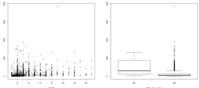
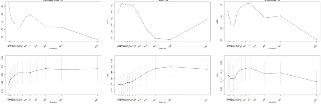
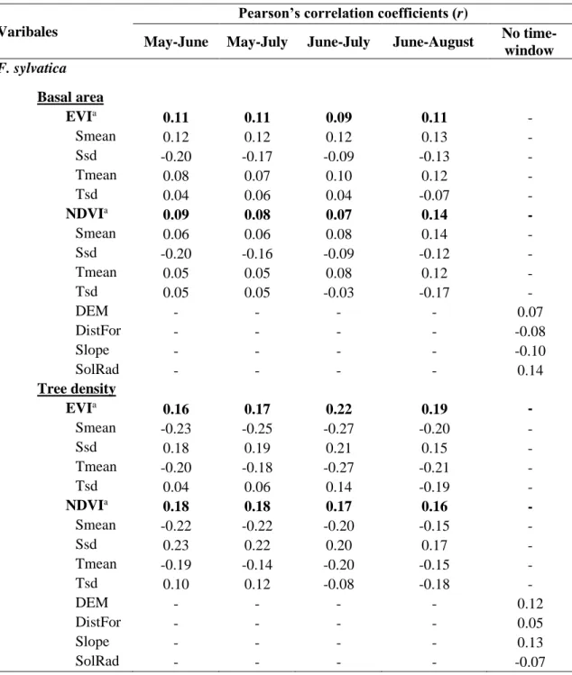
Forest inventories are the raw material providing structural information at the level of the forest plots being investigated, and subsequently data can be summarized to the stand (or higher) level using standard statistical procedures (Brosofske et al. 2014). National forest inventories (NFIs) are designed to acquire information about nationwide forest resources, with the aim of supporting national-level strategic planning and policy development (White et al. 2016). However, given detailed knowledge on forest structure can be also useful to investigate habitat selection by animals deeply related to forest habitat, such as brown bear (Ursus arctos). In this chapter, I aimed to outline a novel and feasible framework to produce spatially explicit forest structural maps, by modeling NFIs stands information, and using time series vegetation indices (i.e., Landsat 5/7 TM/ETM+ satellite images) and environmental characteristic as model predictors. Specifically, I carried out a multi-scale modelling design, accounting for different temporal and spatial scale, under an ensemble modeling

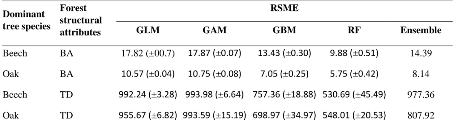
12 approach (Elith and Leathwick 2009, Thuiller et al. 2009). In this framework, I used different statistical algorithms, such as generalize linear model (GLM), generalized additive model (GAM), boosted regression trees (GBM), and random forest (RF), to model trees’ basal area (G; m2_{/ha) and}

number of stems (N; trees/ha), for two target species which dominate the forest in the study area, beech (Fagus sylvatica) and oak (Quercus spp.). Although passive remote sensing images (e.g., Landsat) are generally considered to be poor predictors for tridimensional structure measurements (e.g., Foody et al. 2001) compared to active remote sensing (e.g., LiDAR) images, in this chapter I we described a novel modeling framework that account for multiple scales (spatial and temporal) of analysis to spatially predict tridimensional forest structure with good level of predictive performance, by using easy-to-acquire remote sensing and point-based inventory data.

Chapter III – The importance of forest management strategies in

wildlife conservation: Apennine brown bear’s habitat selection

Forest structural composition largely determines habitat quality for animals, because they may influence the availability and accessibility of resources under many aspects, like selection for rest sites and food (e.g., Hayes and Loeb 2007), exposure to predators (e.g., Baxter et al. 2006) and microclimatic conditions (e.g., Chen et al. 1999). For instance, mature forests characterized by old trees (i.e., higher log’s diameter or basal area) likely provide more resources of food (e.g., hard mast), compared to younger forest characterized instead by smaller trees (i.e., lower log’s diameter and basal area); otherwise, the number of trees (i.e., tree density) of the forest can profoundly affects animal movement (e.g., Caras and Korine 2009), which is especially important not only for flying animals such as birds and bats, but also for larger animals like ungulates (e.g., deer, moose, and wild boars) and carnivores (e.g., wolves, bears and lynxes), which may prefer different forest structures depending on their daily and seasonal activities (i.e., foraging, sheltering, moving to escape from predation or defend the territory). In this chapter, I considered forest horizontal and vertical structure (obtained in Chapter 2) to investigate bear’s space use patterns at two order of selection (Johnson

13 1980), home range (third-order selection) and single forest patch level (fourth-order selection), testing different spatial (i.e., multi-grain analysis; Laforge et al. 2015) and temporal (i.e., seasonal and circadian) scales. At both orders of selection, I used mixed effects logistic regression models (Generalized Linear Mixed Models, GLMMs), treating individual bears as random intercepts, to consider differences in sample size among individuals and autocorrelation of data within individual bears (Gillies et al. 2006). This study confirmed that brown bear is a species related to the forest ecosystem and not limited only to the forest. Looking at the main results, at the home range scale (third-order of selection) the results confirmed the importance of forest like fundamental resource for this brown bear population, related to two main causes: (i) covering by anthropogenic disturbance, highlighted by the selection of continuous forest patch, especially during daily hours in summer (early-summer and late-summer), and (ii) foraging within the forest, highlighted by the increasingly selection for these continuous forested areas mainly in autumn, when there is the peak of hard mast production in the forests. At the single forest patch scale (fourth-order of selection), more evident circadian effects highlight that oak forest selection respect to the beech forest is mainly nocturnal and never diurnal, and this may suggest a trophic rather than covering effect, probably linked to a higher diversity and availability of food.

Chapter IV – Forecasting habitat suitability for Apennine brown

bear under climate change and alternative forest management

scenarios

Forest landscape dynamics result from the complex interaction of driving forces and ecological processes operating on various scales, including large-scale natural disturbances (e.g., wildfires, windthrow), forest management (e.g., trees harvesting), physical environment (e.g., temperature, precipitation and soil), and stand-scale succession and competition processes (e.g., growth, reproduction, seed dispersal and death of the trees). Dynamic landscape-scale models enable us to investigate these complex systems in a quantitative and structured manner (Mladenoff and Baker

14 1999). In this chapter, I investigate how climate change and human forest management can influence the habitat quality and bears-forest habitat relationship. I simulated forest succession dynamics under climate change conditions using spatially explicit landscape-scale vegetation models (i.e., LandClim software; Schumacher et al. 2004; Schumacher and Bugmann 2006) over 50,686-ha study landscape (i.e., Abruzzo-Lazio-Molise National Park, PNALM), using 5 alternatives forest harvesting scenarios. These scenarios were obtained by the combination of different harvesting strategies, and forest-edge treatments, namely S0, S1a, S1b, S2a, and S2b. To forecast future habitat suitability by bears, I used the coefficients estimated in the current habitat selection models at both home range and forest patch-level scales (third and fourth order of Johnson; Chapter 3) in combination with the respective tridimensional structure, composition, and spatial configuration of forest predicted by LandClim’s after 100 years of simulations. In the PNALM, these results suggested that climate change have a substantial impact on forest vegetation: in the next 100 years, LandClim simulations evidenced substantial changes related to the biomass and species composition distribution along altitudinal range, with a gradually conversion of beech dominated forest to oaks domination in all scenarios evaluated. At both orders of selection, I evidenced a general increase of habitat suitability in all the scenarios contemplated compared to the current levels of bear’s habitat suitability. Specifically, at the home range scale (third-order of selection), climate change had a considerable impact on forest species composition compared to the effects of forest harvesting strategies adopted; this trend changes at the forest patch scale (fourth-order of selection), where the different forest strategy adopted increase (or decrease) bear’s habitat suitability.

15

REFERENCES

Abrahms, B., N. R. Jordan, K. A. Golabek, J. W. McNutt, A. M. Wilson, and J. S. Brashares. 2016. Lessons from integrating behaviour and resource selection: Activity-specific responses of African wild dogs to roads. Animal Conservation 19:247–255.

Bates, D., M. Mächler, B. Bolker, and S. Walker. 2015. Fitting linear mixed-effects models using lme4. Journal of Statistical Software 67:1–48.

Baxter, D. J. M., J. M. Psyllakis, M. P. Gillingham, and E. L. O’Brien. 2006. Behavioural response of bats to perceived predation risk while foraging. Ethology 112:977–983.

Benazzo, A., E. Trucchi, J. A. Cahill, P. M. Delser, S. Mona, M. Fumagalli, L. Bunnefeld, L. Cornetti, S. Ghirotto, M. Girardi, L. Ometto, A. Panziera, O. Rota-Stabelli, E. Zanetti, A. Karamanlidis, C. Groff, L. Paule, L. Gentile, C. Vilà, S. Vicario, L. Boitani, L. Orlando, S. Fuselli, C. Vernesi, B. Shapiro, P. Ciucci, and G. Bertorelle. 2017. Survival and divergence in a small group: The extraordinary genomic history of the endangered Apennine brown bear stragglers. Proceedings of the National Academy of Sciences of the United States of America 114:E9589–E9597. Boscagli, G. 1987. Brown bear mortality in central Italy from 1970 to 1984. International Conference

Research and Management 7:97–98.

Brosofske, K. D., R. E. Froese, M. J. Falkowski, and A. Banskota. 2014. A review of methods for mapping and prediction of inventory attributes for operational forest management. Forest Science 60:733–756.

Caras, T., and C. Korine. 2009. Effect of vegetation density on the use of trails by bats in a secondary tropical rain forest. Journal of Tropical Ecology 25:97–101.

Chapron, G., P. Kaczensky, J. D. C. Linnell, M. von Arx, D. Huber, H. Andrén, J. V. López-Bao, M. Adamec, F. Álvares, O. Anders, L. Balčiauskas, V. Balys, P. Bedő, F. Bego, J. C. Blanco, U. Breitenmoser, H. Brøseth, L. Bufka, R. Bunikyte, P. Ciucci, A. Dutsov, T. Engleder, C. Fuxjäger, C. Groff, K. Holmala, B. Hoxha, Y. Iliopoulos, O. Ionescu, J. Jeremić, K. Jerina, G. Kluth, F. Knauer, I. Kojola, I. Kos, M. Krofel, J. Kubala, S. Kunovac, J. Kusak, M. Kutal, O. Liberg, A. Majić, P. Männil, R. Manz, E. Marboutin, F. Marucco, D. Melovski, K. Mersini, Y. Mertzanis, R. W. Mysłajek, S. Nowak, J. Odden, J. Ozolins, G. Palomero, M. Paunović, J. Persson, H. Potočnik, P.-Y. Quenette, G. Rauer, I. Reinhardt, R. Rigg, A. Ryser, V. Salvatori, T. Skrbinšek, A. Stojanov, J. E. Swenson, L. Szemethy, A. Trajçe, E. Tsingarska-Sedefcheva, M. Váňa, R. Veeroja, P. Wabakken, M. Wölfl, S. Wölfl, F. Zimmermann, D. Zlatanova, and L. Boitani. 2014. Recovery of large carnivores in Europe’s modern human-dominated landscapes. Science 346:1517–1519.

Chen, J., S. C. Saunders, K. D. Brosofske, G. D. Mroz, T. R. Crow, R. J. Naiman, J. F. Franklin, and B. L. Brookshire. 1999. Microclimate in forest ecosystem and landscape ecology: Variations in local climate can be used to monitor and compare the effects of different management regimes. BioScience 49:288–297.

Ciucci, P., and L. Boitani. 2008. The Apennine brown bear: A critical review of its status and conservation problems. Ursus 19:130–145.

16 abundance of the remnant Apennine brown bear population using multiple non invasive genetic data sources. Journal of Mammalogy 96:206–220.

Ciucci, P., E. Tosoni, G. Di Domenico, F. Quattrociocchi, and L. Boitani. 2014. Seasonal and annual variation in the food habits of Apennine brown bears, central Italy. Journal of Mammalogy 95:572–586.

Colangelo, P., A. Loy, D. Huber, T. Gomerčić, A. Vigna Taglianti, and P. Ciucci. 2012. Cranial distinctiveness in the Apennine brown bear: Genetic drift effect or ecophenotypic adaptation? Biological Journal of the Linnean Society 107:15–26.

Czetwertynski, S. M., M. S. Boyce, and F. K. Schmiegelow. 2007. Effects of hunting on demographic parameters of American black bears. Ursus 18:1–18.

Dickson, B. G., J. S. Jenness, and P. Beier. 2005. Influence of vegetation, topography, and roads on cougar movement in southern California. Journal of Wildlife Management 69:264–276.

Elith, J., and J. R. Leathwick. 2009. Species distribution models: ecological explanation and prediction across space and time. Annual Review of Ecology, Evolution, and Systematics 40:677–697.

Falcucci, A., P. Ciucci, L. Maiorano, L. Gentile, and L. Boitani. 2009. Assessing habitat quality for conservation using an integrated occurrence-mortality model. Journal of Applied Ecology 46:600–609.

Foody, G. M., M. E. Cutler, J. McMorrow, D. Pelz, H. Tangki, D. S. Boyd, and I. Douglas. 2001. Mapping the biomass of Bornean tropical rain forest from remotely sensed data. Global Ecology and Biogeography 10:379–387.

Gervasi, V., L. Boitani, D. Paetkau, M. Posillico, E. Randi, and P. Ciucci. 2017. Estimating survival in the Apennine brown bear accounting for uncertainty in age classification. Population Ecology 59:119–130. Springer Japan.

Gillies, C. S., M. Hebblewhite, S. E. Nielsen, M. A. Krawchuk, C. L. Aldridge, J. L. Frair, D. J. Saher, C. E. Stevens, and C. L. Jerde. 2006. Application of random effects to the study of resource selection by animals. Journal of Animal Ecology 75:887–898.

Hayes, J. P., and S. C. Loeb. 2007. The influences of forest management on bats in North America. Pages 207–236 in. Bats in Forests: Conservation and Management. eds M.J. L. John Hopkins University Press, Baltimore, MD.

Johnson, D. H. 1980. The comparison of usage and availability measurements for evaluating resource preference. Ecology 61:65–71.

Laforge, M. P., E. Vander Wal, R. K. Brook, E. M. Bayne, and P. D. McLoughlin. 2015. Process-focussed, multi-grain resource selection functions. Ecological Modelling 305:10–21.

Levin, S. A. 1992. The problem of pattern and scale in ecology: The Robert H. MacArthur award lecture. Ecology 73:1943–1967.

Lorenzini, R., M. Posillico, S. Lovari, and A. Petrella. 2004. Non-invasive genotyping of the endangered Apennine brown bear: A case study not to let one’s hair down. Animal Conservation 7:199–209.

17 Loy, A., P. Genov, M. Galfo, M. G. Jacobone, A. V. Taglianti, P. Genov, M. Galfo, M. G. Jacobone, and A. V. Taglianti. 2008. Cranial morphometrics of the Apennine brown bear (Ursus arctos

marsicanus) and preliminary notes on the relationships with other southern European

populations. Italian Journal of Zoology 75:67–75.

Mace, R. D., J. S. Waller, T. L. Manley, L. J. Lyon, and H. Zuuring. 1996. Relationships among grizzly bears, roads and habitat in the Swan Mountains Montana. The Journal of Applied Ecology 33:1395–1404.

Maiorano, L., L. Chiaverini, M. Falco, and P. Ciucci. 2019. Combining multi-state species distribution models, mortality estimates, and landscape connectivity to model potential species distribution for endangered species in human dominated landscapes. Biological Conservation 237:19–27.

Manly, B. F. J., L. Mcdonald, D. Thomas, T. L. McDonald, and W. P. Erickson. 2002. Resource selection by animals: Statistical design and analysis for field studies. 2nd ed. Volume 1. Kluwer Academic Publishers, Dordrecht, Netherlands. Merkle.

Di Marco, M., and L. Santini. 2015. Human pressures predict species’ geographic range size better than biological traits. Global Change Biology 21:2169–2178.

Mayor, S. J., D. C. Schneider, J. A. Schaefer, and S. P. Mahoney. 2009. Habitat selection at multiple scales. Écoscience 16:238–247.

McGarigal, K., H. Y. Wan, K. A. Zeller, B. C. Timm, and S. A. Cushman. 2016. Multi-scale habitat selection modeling: A review and outlook. Landscape Ecology 31:1161–1175.

Mladenoff, D. J., and W. L. Baker. 1999. Development of forest and landscape modeling approaches. Pages 1–13 in. Mladenoff, D.J., Baker, W.L. (Eds.), Spatial Modeling of Forest Landscape Change: Approaches and Applications. Cambridge University Press, Cambridge, UK.

Ordiz, A., J. Kindberg, S. Sæbø, J. E. Swenson, and O. G. Støen. 2014. Brown bear circadian behavior reveals human environmental encroachment. Biological Conservation 173:1–9.

Posillico, M., A. Meriggi, E. Pagnin, S. Lovari, and L. Russo. 2004. A habitat model for brown bear conservation and land use planning in the central Apennines. Biological Conservation 118:141– 150.

Randi, E., L. Gentile, G. Boscagli, D. Huber, and H. U. Roth. 1994. Mitochondrial DNA sequence divergence among some west European brown bear (Ursus arctos L.) populations. Lessons for conservation. Heredity 73:480–489.

Schumacher, S., and H. Bugmann. 2006. The relative importance of climatic effects, wildfires and management for future forest landscape dynamics in the Swiss Alps. Global Change Biology 12:1435–1450.

Schumacher, S., H. Bugmann, and D. J. Mladenoff. 2004. Improving the formulation of tree growth and succession in a spatially explicit landscape model. Ecological Modelling 180:175–194. Thuiller, W., B. Lafourcade, R. Engler, and M. B. Araújo. 2009. BIOMOD - a platform for ensemble

forecasting of species distributions. Ecography 32:369–373.

18 reproductive traits in the Apennine brown bear population. Ursus 28:105–116.

White, J. C., N. C. Coops, M. A. Wulder, M. Vastaranta, T. Hilker, and P. Tompalski. 2016. Remote sensing technologies for enhancing forest inventories: A review. Canadian Journal of Remote Sensing 42:619–641.

Zunino, F., and S. Herrero. 1972. The status of the brown bear (Ursus arctos) in Abruzzo National Park, Italy, 1971. Biological Conservation 4:263–272.

19

Chapter I

Unveiling differences in scale-dependent habitat selection of

the Apennine brown bear using multi-grain, multi-order

resource selection functions

Matteo Falco, Luigi Maiorano, and Paolo Ciucci

Sapienza University of Rome, Dept. of Biology and Biotechnology “Charles Darwin”, Viale dell’Università 32, Roma 00185, Italy

20

INTRODUCTION

Habitat selection is a dynamic process that depends on the different spatial and temporal scales of the environment in which the species live (Levin 1992; Mayor et al. 2009; McGarigal et al. 2016). Habitat is characterized by a multidimensional structure in which species perceive and respond to their surroundings across a range of spatial scales, also defined as scales of domain (Wiens 1989, Kotliar and Wiens 1990, Levin 1992). Identifying the scale of domain at which habitat selection operates is therefore fundamental to understand unambiguously the relative risk or rewards animals obtain by selecting a given resource at an adequate scale of investigation (Roland and Taylor 1997; Holland et al. 2004). In this context, multiscale habitat analysis provides important theoretical insight into ecological patterns and processes, and facilitates effective conservation and management (Benítez-López et al. 2017; Pimenta et al. 2018). The concept of scale in ecology has been widely used to describe a variety of related concepts (Wiens 1989, Levin 1992, Schneider 2001, McGarigal et al. 2016b), among which both extent and grain are of particular operational value (Levin 1992, Hall et al. 1997, Morrison and Hall 2002, Mayor et al. 2009, McGarigal et al. 2016b). While the former refers to the geographic and temporal constraint in which resources are effectively available to animals, the latter refers to the resolution at which an animal responds to the environmental heterogeneity, generally measured as the radius within which animals perceive and respond to environmental predictors [also referred as ‘grain response’ or ‘characteristic scale’ (Addicott et al. 1987; Holland et al. 2004)]. Nevertheless, even though habitat selection is increasingly recognized as a multi-scale process (Holland et al. 2004, Mayor et al. 2009, Laforge et al. 2015, McGarigal et al. 2016a), habitat selection studies still very often consider a single extent and a fixed grain (Mayor et al. 2009), thereby failing to identify changes in habitat selection across ecological domains (Wiens 1989). A multi-scale approach involves the explicit consideration of explanatory variables measured at more than one spatial and/or temporal scale, with variations on how to choose and analyze relationships across scales (McGarigal et al. 2016a). In this context, Johnson's (1980) hierarchical framework to investigate habitat selection, though potentially confused with a multi-scale approach

21 (Wheatley and Johnson 2009), can been conveniently adopted to define given spatial and temporal extents when adopting use vs availability study designs to assess habitat selection (Mayor et al. 2009, Gaillard et al. 2010). In some circumstances, temporal scale may be more important than spatial scale (Fahrig 1992), because differences between seasonal and daily decisions can affect spatial decisions in choosing the home range within landscape (i.e., second-order of selection; Johnson 1980), and high-suitable patches within home range (i.e., third-order of selection; Johnson 1980).

There are numerous analytical approaches and statistical modelling methods available for developing multiscale habitat selection modeling. In this sense, RSFs framework can be easily adapted for modeling different spatial scales both in terms of extent and grain, and temporal scales (i.e., the duration and resolution of observations in time). Similar to other statistical methods, such as species distribution models (SDMs; Guisan and Zimmermann 2000) and Ecological Niche factor Analysis (ENFA; Hirzel et al. 2002), RSFs have been widely used in studies of wildlife habitat selection (Boyce and McDonald 1999, Manly et al. 2002), and they serve an applied role of converting ecological niche relationships in environmental space into gradients of predicted habitat suitability across geographic space (Hirzel and Le Lay 2008).

Large carnivores with their wide movement ranges and large spatial requirements are a good model for understanding how scales influence resources selection and space use of animal populations, particularly in human dominated landscapes. A large carnivore species recognized for its remarkable plasticity to persist in human-altered landscapes is brown bear (Ursus arctos) (Cozzi et al. 2016). Brown bear distribution encompass the majority habitats of the Holarctic region (North America and Eurasia), but its optimal habitat is considered to be human-less areas with a mosaic of early-seral staged forests and natural openings in proximity to forest stands that provide day beds and hiding cover (Herrero 1972, Blanchard 1983, Hamer and Herrero 1987) located in dense vegetation and steeper terrain (Moe et al. 2007, Elfström et al. 2008, Ordiz et al. 2011). Nonetheless, different factors could influence spatial or temporal habitat segregation among bears, such as innate sexual differences, age classes, and individual temperament (Martin and Réale 2008, Ellenberg et al. 2009);

22 for instance, female bears with small cubs mast prioritize offspring security and frequently select lower-quality habitat characterized by a more human dominated landscapes in order to avoid males (Elfström et al. 2014b, Lamb et al. 2016). This bear’s capacity to adapt its spatiotemporal niche to human presence becomes a fundamental trait for its persistence in human dominated environments, and knowledge on such adaptations is essential for effective and long-term conservation planning (Ordiz et al. 2012).

Living surrounded by a very high human-dominated landscape in central Italy, Apennine brown bear (Ursus arctos marsicanus; Altobello 1921) represent the last remnant of an autochthonous population, isolated from other European bear populations for at least 1,500 years (Benazzo et al. 2017). Most of the current core distribution of Apennine brown bear is constituted by the Abruzzo-Lazio-Molise National Park (PNALM), which comprises relatively ideal habitat conditions for bears compared to other regions of Italy. Human infrastructures, including settlements and roads, have been historically present in the area at low densities, and multiple use practices (e.g. tourism, livestock husbandry, silvicultural activities) have been traditionally allowed in the park (Mancinelli et al. 2019). This bear population is facing serious risks of extinction due to its persistent small size and reduced genetic variability (Ciucci et al. 2015, Benazzo et al. 2017, Gervasi and Ciucci 2018), and needed immediate proactive conservation measures (Ciucci and Boitani 2008).

To achieve this goal, previous habitat-modelling applications were conducted at landscape scale to evaluate, for instance, the effectiveness of the national and regional networks of protected areas (Posillico et al. 2004), potential ecological traps (Falcucci et al. 2009) and corridors linking the core distribution (i.e., distribution range of female bears producing cubs; Ciucci et al. 2017) with the other surrounding suitable areas within its historical distribution range (Maiorano et al. 2019). Nonetheless, habitat selection analysis developed using a multi-scale approach to evidence bears-habitat relationships within its core distribution is not yet conducted. Assessing new ecological information over this population accounting for multiple spatial and temporal scales become critical for achieving

23 evidenced-base habitat management schemes, and enhancing conservation efforts for the demographic expansion of this unique brown bear population.

In this study, I used Global Positioning System (GPS) locations recorded from 11 adult females (2006-2010) to model bears’ habitat selection based on multi-grain resource selection functions (MRSF) study design. My objectives are to model the home range space-use pattern by bears associated to available resources at landscape scale (e.g. second-order of selection; Johnson 1980) and within home range (e.g. third-order of selection; Johnson 1980), contemplating a set of environmental and anthropogenic predictors, and investigate bears’ behavioral responses to seasonal and circadian effects, at both population and individual level. My working hypotheses are that (i) resource selection by female bears is related to factors describing human inaccessible habitats, and (or) attraction of foods available in the forest ecosystem. In addition, (ii) habitat selection by female bears could be spatial scale-dependent, and changes in habitat selection across ecological domains (Wiens 1989) may be revealed by accounting for multiple observational scales (including extent and grain; Wheatley and Johnson 2009); accordingly, I expect that human-risk perceived by female bears is greater in choosing home ranges in the landscape (second-order), compared to patch-level habitat selection within home range (third-order); nonetheless, at the third-order, temporal scale may highlight differences in anthropogenic features response, similar to the seasonal and circadian human avoidance pattern found by Mancinelli et al. (2019) for wolves in the same study area. Finally, (iii) habitat selection at population level may hide a high-variability in selection pattern among individuals (Gill et al. 2001, Elfström et al. 2014b), and spatiotemporal variation in the selection pattern for anthropogenic features may be in part explained by functional responses, occurring when individuals change their preference as a function of the availability of particular habitat features (Mysterud and Ims 1998, Hebblewhite and Merrill 2008).

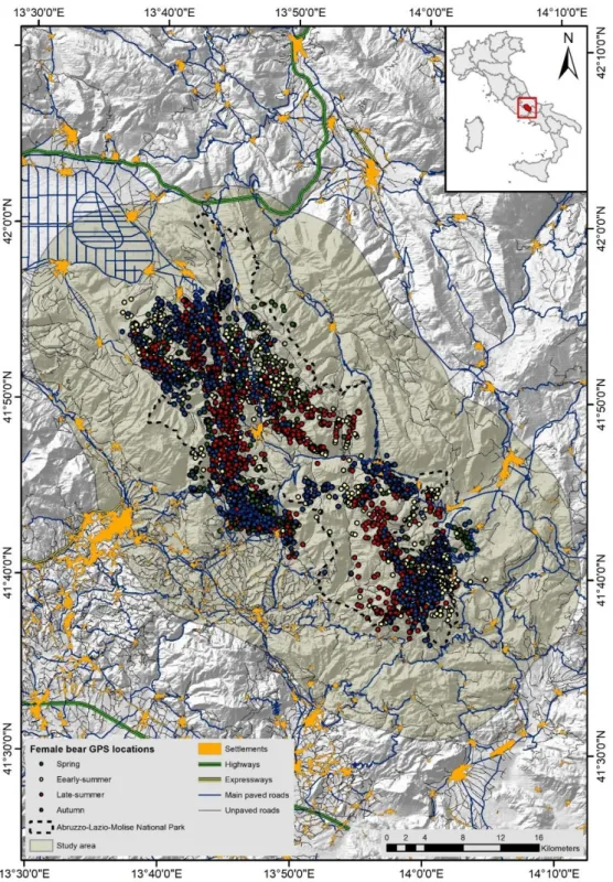
METHODS Study area

24 I defined the study area as the area encompassed within a 10 km buffer (see Model development below) around the composite 100% MCP calculated using all Global Positioning System (GPS) locations of radio-collared female bears included in the analysis (Fig. 1). The 656.8 km2 study area comprises therange of reproductive Apennine female bears in the Abruzzo Lazio and Molise National Park (PNALM) and adjacent areas (Ciucci et al. 2017). Altitude ranges from 145 to 2278 m. a. s. l., progressing from gentle slopes dominated by cultivated lands and human settlements to typically mountainous terrain, mainly covered by forests interspersed with pastures, meadows, and alpine prairies. Forests cover 68.6% of the study area, mainly beech (Fagus sylvatica) and oak (mainly

Quercus cerris and Q. pubescens), followed by open fields and shrublands. Agriculture is scarce and

highly localized along valley bottoms and close to human settlements. The study area features a relatively low paved road density (45.3 km/100 km2_{) and a few, scattered villages (Table 1). Human}

presence (27.1±16.7 inhabitants/km2) and activities markedly increase during summer, mostly due to tourism and livestock grazing (Mancinelli et al. 2018).

Data collection

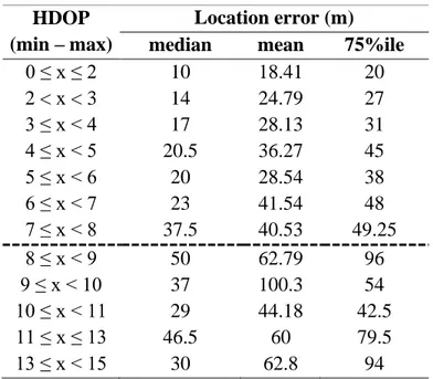
From 2005 to 2010, I live-trapped bears and deployed Global Positioning System (GPS) collars (Televilt Tellus GSM-VHF, and Vectronic GPS Plus) on 19 adult (≥ 4 years) bears (8 males and 11 females). I focused the habitat analysis on adult female bears only due to their critical demographic role (Knight and Eberhardt 1985, Wiegand et al. 1998, Boyce et al. 2001, Nielsen et al. 2006). Stationary collars posted at fixed points (n = 100) within the study area had an average location error of 24.7m (±16.3m SD) (Mancinelli et al. 2019). Collars deployed on bears were programmed to acquire one location every hour (i.e., 24 relocations/day) for 10 days a month, followed by one location every 4−6 hours for the rest of the month. For the scope of the analysis, I subsampled all locations at an equal rate of 4 locations/day. I limited the analyses to locations collected during the active period, defined according to the median dates of den exit and entrance of adult females in this bear population (7 Mar and 23 Nov, respectively; Ciucci et al. 2012). Observed acquisition rates of GPS locations ranged 73.1−98.6% for individual bear (𝓍 ̅ =86.7±9.2%; Supplementary Table S1). To

25 enhance the quality of GPS locations used in the analyses (Lewis et al. 2007), I retained all GPS locations acquired with: (i) 3 satellites, but with horizontal dilution of precision (HDOP) < 8 (location error: 𝓍̅=23.3±33.8 m), and (ii) ≥ 4 satellites (Supplementary Table S2 and Fig. S1). At the third order of selection, to account for seasonal variation in habitat selection I considered 4 periods according to the local seasonality in bear key foods (Ciucci et al. 2014): spring (March−May), early-summer (June−July), late-summer (August−September), and fall (October−23 November). If a bear had been tracked for more than one year, I did not include seasonal duplicates but selected the season with the highest number of acquired locations. The final dataset comprised a total of 9,380 GPS locations for 11 adult female bears (38 bear-seasons; Supplementary Table S1).

Habitat variables

To account for resource selection by adult female bears, I considered a set of 11 environmental, topographic and anthropogenic variables in a GIS environment (ArcMap v. 10.2; Environmental Systems Research Institute, ESRI, Redlands, CA, USA). I obtained land cover layers from the regional Corine Land Cover (CLC) V level and forest type vector maps, at 1:10,000 scale, from Regional administrations (http://geoportale.regione.abruzzo.it/; https://geoportale.regione.lazio.it/;

http://www.geo.regione.molise.it/). I combined the original land cover categories into four classes: forests (including broadleaf and coniferous forest), open fields (including pastures, meadows, and alpine prairies), shrublands, and cultivated lands, the latter mostly characterized in the study area by non-intensive agriculture. To account for topographic variables, I used a digital elevation model (DEM; 10x10 m cell-size) obtained by the Italian Military Geographic Institute (IGM), from which I computed hillshade, slope and its standard deviation (Spatial Analyst Tool; ArcMap v. 10.2, ESRI). Hillshade is a orographic measure of solar exposition indicating the average amount of shade at any pixel (ranging from 0 to 255; Ciarniello et al. 2005), whereas the standard deviation of the slope is a measure of terrain roughness (Maiorano et al. 2015).

Anthropogenic variables included the Euclidean distance to the closest road and settlement edge. The former was derived combining the De Agostini-GeoNext and TeleAtlas databases (updated to 2003),

26 the latter by the National Institute of Statistics (ISTAT 2011). I classified roads as either paved roads or unpaved roads, both accessible by vehicles; although I lacked measures of traffic volumes, I expected a markedly lower vehicle traffic on unpaved roads. Furthermore, to eliminate all road segments really inaccessible by vehicles, I integrated the available road network GIS-layer with the trails network collected by the Forest service, during the LIFE-project ARCTOS (http://www.parcoabruzzo.it/pagina.php?id=201), within the same study area. All variables were calculated or re-sampled (i.e., DEM) with a common origin and 20x20 m cell size resolution. For each variable, I used the focal statistics tool in ArcGIS (ESRI) to ran a map-algebra focal function over the entire study area; to this aim, and to allow a multi-grain approach, I used moving windows of different radii to model alternative grain sizes (see Optimized multi-grain analysis).

Multi-grain Resource Selection Functions

Based on an use-availability design (Manly et al. 2002), I developed two multi-grain resource selection functions (MRSFs; Laforge et al. 2015), one contrasting habitat features at the landscape (study area) extent with those within the bears’ annual home ranges (i.e., second-order selection,

sensu Johnson 1980), and one contrasting habitat features at bears’ GPS locations with those within

their corresponding seasonal home ranges (i.e., third-order selection; Johnson 1980). At both orders of selection, I fitted a mixed-effects logistic regression model (Generalized Linear Mixed Models, GLMMs) using the ‘lme4’ R package (Bates et al. 2015). I treated individual bears as random intercepts, to take into account differences in sample size among individuals and autocorrelation of data within individual bears (Gillies et al. 2006). I standardized each variable by subtracting the mean value from each observation and dividing by its standard deviation to allow comparison of covariates’ effects and to improve model convergence (Zuur et al. 2009). I then calibrated GLMMs including all combinations of variables (dredge function in ‘MuMIn’ R package; Barton 2018), and performed model selection using the sample-size corrected Akaike’s Information Criterion (AICc; Burnham and

Anderson 2002). I averaged estimates based on model weights (‘MuMIn’ R package; Barton 2018) limited to models whose AICc value was ≤ 2 from the most supported model (Burnham and Anderson

27 2002). Finally, I estimated unconditional standard errors and 95% confidence intervals for averaged coefficients, the latter considered significant when they did not include the 0 value. I also determined the relative importance of each covariate by summing the AICc weights of all models including a

given covariate (Burnham and Anderson 2002). As few candidate models receive Akaike weights > 0, I did not incur the risk of spurious results from averaging parameter estimates of too many models with low weight (Grueber et al. 2011). Finally, using ‘MuMIn’ R package (Barton 2018), I quantified the proportion of variance explained by the averaged models, calculating the coefficient of determination (R2; Nakagawa et al. 2017), distinguishing between the variance explained by the fixed effects (i.e., marginal, 𝑅_(𝑚)2 ) and the variance explained by both fixed and random effects (i.e., conditional form, 𝑅_(𝑐)2 ). Because these analysis was based on a relatively small sample size, I accounted for overfitting problems (Anderson 2008) by considering models with low complexity and a limited number of covariates, and by reducing the number of models to be compared. In addition, the aim of these models was not to make predictions of habitat use by bears outside the study area, further reducing the negative effects of potential overfitting (Zellner et al. 2001, Anderson 2008).

To assess the calibration power of the final model (i.e., how much model predictions differed from a random expectation; Vaughan and Ormerod 2005), I used k-fold cross-validation (k=10) randomly splitting the dataset into 10 bins. By removing 1 bin at time, successively used as a validation set, I used the remaining data (training set) to estimate the MRSF coefficients, and I repeated the procedure for all the remaining bins. For each training set, instead of using fixed classes, I partitioned the predicted MRSF values into continuous bins calculated through a moving window of width W (W = 1/10 of the highest predicted value) (Hirzel et al. 2006). For each continuous bin, I first calculated the frequency of evaluation points falling in each class respect the total number of points (predicted frequency), and then the frequency of the predicted values of each class compared to the total amount of training points (expected frequency). Finally, I computed the Spearman rank correlation coefficient, also called “continuous Boyce index” (hereafter Boyce index, Bcont(W); Hirzel

28 to 1, where positive values indicate both high predictive model’s performance and deviation from randomness (i.e., valuesclose to zero), while negative values indicate an incorrect model. The whole validation procedure was repeated for 100 times.

At the third-order selection, to investigate circadian effects on seasonal selection patterns basis I distinguished between daily and night GPS locations using the solarpos function (‘maptools’ R package; Bivand et al. 2016).

Optimized multi-grain analysis

To identify the optimal grain size for each environmental variable, I used the grain optimization procedure developed by Laforge et al. (2015). Within a resource selection function framework, this procedure involves assessing the most parsimonious grain size of a given variable by changing the grain size of one variable at the time, conditionally on the other covariates. Specifically, for one variable at the time, I compared the model with and without the focal variable measured at a given grain size using AICc; that is (Laforge et al. 2015):

𝛥𝐴𝐼𝐶_𝑐𝑣𝑎𝑟𝑖𝑎𝑏𝑙𝑒(𝑥) = 𝐴𝐼𝐶_{𝑐 𝑔𝑙𝑜𝑏𝑎𝑙 𝑚𝑜𝑑𝑒𝑙}− 𝐴𝐼𝐶_{𝑐 𝑔𝑙𝑜𝑏𝑎𝑙 𝑚𝑜𝑑𝑒𝑙−𝑣𝑎𝑟𝑖𝑎𝑏𝑙𝑒(𝑥)}

Using the ‘MuMin’ R package (Barton 2018), and by repeating the procedure above for different grain sizes, I then plotted ΔAICc versus grain sizefor each variable to identify the most

parsimonious (i.e., minimum ΔAICc values) grain for a given variable (see Laforge et al. 2015 for

more details). As this procedures potentially allows to detect different selection patterns for a given variable at different grain sizes (i.e., coefficients of different sign; Ciucci et al., 2018; Laforge et al., 2015), in these cases I included the variable twice in the in the final, multi-grain model using both grain sizes, provided these were not correlated (see below). To identify the values and range of grain sizes to be assessed for each variable, I followed Zeller et al. (2014) by first fitting a Pareto function to the adult female bears’ step-length distribution, and then by dividing this function into quintiles (‘POT’ and ‘adehabitatLT’ R packages; Calenge 2006, Ribatet and Dutang 2016) (see Supplementary material for further details). The entire grain-size optimization procedure was repeated to develop MRSF models both at the second and the third order of selection (Supplementary Fig. S2-S11).

29

Habitat selection at the landscape scale (second-order selection)

To model resource selection at the landscape extent I followed a design II (Thomas and Taylor 2006) by quantifying habitat use of each adult female bear by randomly sampling its annual home range (100% Minimum Convex Polygon, MCP) at a density of 100 points/km2, and measuring availability at the population level by randomly sampling 10,000 points within the study area, defined as the overall MCP of all adult female bears GPS locations and including a 10-km external buffer, (i.e., the upper limit of the 95% confidence interval of each adult female bear’s annual MCP diameter). After checking for collinearity among covariates, including those entered in the model with >1 grain size, I discarded first altitude and distance from paved roads as these were correlated with distance from settlements (r>0.7; Supplementary Table S3), and then open field to reduce multicollinearity (VIF<3; Supplementary Table S4). I therefore retained a total of 8 uncorrelated variables in the final model.

Habitat selection within the home range (third-order selection)

To model seasonal resource selection at the home range extent, I followed a design III (Thomas and Taylor 2006) by using adult female bear’s seasonal GPS locations to represent use and randomly sampling locations within their seasonal home ranges (100% MCP) at a density of 100 points/km2 to measure availability. After checking for collinearity among covariates, including entered in the model with >1 grain size, I discarded open fields and altitude as these were correlated with forest and distance from settlements (VIF>3; Supplementary Table S9). I therefore retained a total of 8 uncorrelated variables in the final models.

To test my hypothesis of a circadian effect on seasonal habitat selection at the third-order, I used Latent Selection Differences (LSD) functions (Czetwertynski et al. 2007). Similar to an RSF approach, this method allows a direct comparisons of habitat selection between two groups of interest (in my case, day vs night), producing quantifiable measurements of the relationships’ strength (Czetwertynski et al. 2007, Latham et al. 2011). A fundamental assumption of LSD is that all

habitat-30 types should be equally available to both groups of interest, an assumption that reasonably holds on a seasonal basis in my case.

Functional response in habitat selection

To investigate functional responses toward anthropogenic features, the relatively small sample size of adult female bears (9 ≤ n ≤ 10) did not allow us to contemplate models including individual ID both as an intercept and a random coefficient (e.g., Gillies et al. 2006). Instead, following the procedure described above, I used generalized linear models (GLMs; R Development Core Team, 2019) to develop individual, seasonal MRSFs at the third order selection for each adult female bear. Successively, I used generalized additive models (GAMs; ‘mgcv’ R package; Wood 2011), to assess individual responses by fitting individual MRSFs coefficients of anthropogenic features as a function of their availability within each adult female’s the home range. I then used an information-theoretic approach to perform model selection, comparing each model calibrated (i.e., anthropogenic model) with the respective intercept-only model (i.e., null-model); comparing AICc values of the two models,

I assessed statistical significance of the functional response when the AICc value of the former

(anthropogenic model) is lower than the latter (null-model). Finally, I calculated the variance explained by the model (R2) as a measures of the strength of the relationship between model and the dependent variable (Zuur et al. 2009).

RESULTS

Habitat selection at the landscape scale

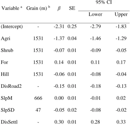
At the study area extent, the most parsimonious grain for all variables was the maximum I modelled, except for the variables mean slope and roughness (47 m and 666 m, respectively; Table 2). I averaged the global model without slope (wi=0.59) and the global model (wi=0.35), and the

averaged model fitted the data reasonably well (Bcont(W)=0.90±0.06). The variance explained by both

fixed and random effect (𝑅_(𝑐)2 = 0.50) was higher than the variance explained by the fixed effects alone (𝑅_(𝑚)2 = 0.40).

31 When locating their home ranges at the landscape scale, adult female bears selected areas with higher forest cover but avoided cultivated lands, shrubland, areas closer to human settlements and less exposed sites. They also selected areas closer to unpaved roads and for relatively even terrain at a small grain (Table 3).

Habitat selection within the home range

Within the home range, the most parsimonious grain size varied across covariates, ranging from 47 m (forest, shrubland) to 1531 m (roughness) and, on average, was consistently small across seasons, with few exceptions (e.g., shrubland in early summer; Table 2). The global model was the most supported in early-summer (Bcont(W) = 0.82±0.07), late-summer (Bcont(W) = 0.83±0.07), and

autumn (Bcont(W) = 0.74±0.21); in spring, however, the model without settlements was similarly

plausible and was averaged with the global model (Bcont(W) = 0.73±0.09). Whereas the variance

explained by the global models varied among seasons, within each season the variance explained by both fixed and random effect (0.15 ≤ 𝑅_(𝑐)2 ≤ 0.28) was consistently higher than the variance explained by the fixed effect alone (0.07 ≤ 𝑅_(𝑚)2 ≤ 0.19).

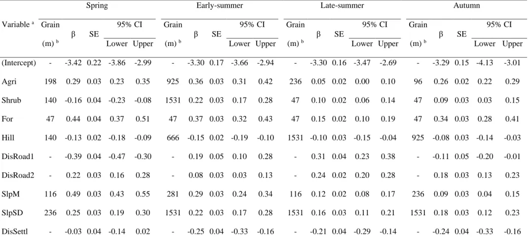
I detected relevant seasonal (Table 4) and circadian (Table 5) effects in habitat selection by adult female bears at the home range extent. Consistently across seasons, adult female bears selected proxies of food and cover (agriculture and forest cover) or of inaccessibility by humans (i.e., steeper slopes, rough terrain, and greater distance from dirt roads), while avoiding less exposed sites (Table 4). However, consistently across seasons, forest cover was exceedingly selected during daylight hours compared to the night, whereas agricultural fields were increasingly selected during the night in spring and fall (Table 5). Areas further from dirt roads were especially selected during daylight hours, and so were steeper slopes in three out of four seasons (Table 5). Shrub lands were avoided by adult female bears in spring but were selected in the other seasons (Table 4), with a greater use during daylight hours in early and late summer (Table 5). Areas closer to main paved roads were avoided in early and late summer but increasingly used in spring and fall, whereas areas closer to human

32 settlements were increasingly used during early and late summer (Table 4), both without apparent circadian effects (Table 5).

Functional responses towards anthropogenic features

At the individual level, adult female bears expectedly showed high variability in their third-order, seasonal habitat selection (Supplementary Tables S11−S14 and Fig. S12). Most parsimonious MRSF models at the individual level had 𝑅2 _{values largely differing across individuals and seasons}

(spring: 0.15 ≤ 𝑅2 ≤ 0.68, n=9; early-summer: 0.05 ≤ 𝑅2 ≤ 0.63, n=9; late-summer: 0.21 ≤ 𝑅2 ≤ 0.33, n=10; autumn: 0.11 ≤ 𝑅2 ≤ 0.57; n=10). However, selection patterns shared by all or most adult female bears consistently reflected (a) avoidance of areas closer to dirt roads (spring and late summer), and (b) selection for forest cover (spring and early summer), agricultural fields (early summer, late summer and fall), shrub lands (late summer), steeper slopes (spring and late summer), rough terrain (late summer), and sites less exposed to sunlight (spring) (Supplementary Fig. S12).

Based on individual, seasonal MRSFs, I detected functional responses by adult female bears toward anthropogenic features at the third-order selection, in particular paved (Fig. 2A-B) and unpaved (Fig. 3A-B) roads, both in spring and late summer, and settlements in autumn (Fig. 4). I failed to detect a functional response towards the same anthropogenic features in the other seasons (i.e., AICc(null model) > AICc(anthropogenic model); 3.64% ≤ R2 ≤29.8%). During spring, adult

female bears showed strong avoidance (i.e., positive s) of areas closer to paved roads at high road densities (i.e., low average distance from roads within the home range), but avoidance waned at intermediate and low road densities (R2sp=0.42; Fig. 2A); similarly, during summer, avoidance of

areas closer to paved roads was highest at intermediate road densities and waned as road density decreased (R2

ls=0.87; Fig. 2B). Contrarily, adult female bears increasingly avoided areas closer to

unpaved roads at decreasing road densities within their home range, consistently in spring and late summer (R2sp=0.52 and R2ls=0.49, respectively), even they never selected for areas close to unpaved

roads also where these occurred at higher densities (Fig. 3A-B). Finally, limited to the autumn, adult female bears selected for areas closer to settlements where these occurred at higher density (i.e., a

33 lower mean distance from settlements within the home range), but selection rapidly waned at decreasing settlement density (R2au=0.79, Fig. 4).

DISCUSSION

My findings revealed a hierarchical and scale-sensitive process, according to the spatial (i.e., extent and grain) and temporal (i.e., seasons and circadian effect) scales investigated. Whereas land cover and anthropogenic variables are key-factors determining habitat selection by female bears at the landscape scale (i.e., second-order), orographic characteristics become crucial in the habitat selection at the patch-level (i.e., third-order). Compared to the landscape, I found that habitat selection at the home range scale by adult female bears indicates plausible changes in ecological domains. The heavily selection for further distances from human settlements and agricultural fields (i.e., second-order), particularly during the night (i.e., third-second-order), may indicate a trade-off between the risk of frequenting human-associated land covers and the attraction of foods available at lower altitudes, following phenology of grasses and forbs whose consumption by Apennine bears is highest in spring and fall (Ciucci et al. 2014). Because of the more accessible vegetable foods that can be forage, and according to seasonal food availability, bears commonly utilize human-derived foods near settlements (Elfström et al. 2014; Zarzo-Arias et al. 2018) and cultivate lands (Swenson et al. 1999, Große et al. 2003, Roever et al. 2008a, b). For bears living in densely populated countries, this might correspond to understanding the main sources of human-caused mortality or compromised fitness, and accordingly assess their spatial variation across scales. Actually, the ‘scale’ factor has been little considered in the previous Apennine brown bear’s habitat selection studies. For instance, Posillico et al. (2004) tempt to capture bear-habitat relationship at landscape scale accounting for one single-coarse grain resolution (5x5km grid-cell), while in following studies (Falcucci et al. 2009, Maiorano et al. 2015, 2019) habitat selection models were performed by using a smaller grain size (i.e., 400 m) and accounting for a larger set of predictor variables. Overall, brown bear’s presence in the central Apennine has been positive associated with elevation and steeper areas rich in broadleaf forests, while negative associated to roads (both paved and unpaved), human density, shrubs, and cultivated fields.

34 Despite there were an increasingly use of more sophisticated analysis through the time, going from ENFA analysis (Falcucci et al. 2009) to SDMs (Maiorano et al. 2015, 2019), as well as the use of ever more high-resolution variables, these findings partially explain the occurring bears-habitat relationships that instead emerge when resource selection is investigated by accounting for multiple observational scales.

Although limited by a relatively small number of GPS-collared female bears, my study represents the first investigation to describe bear’s responses to habitat resources accounting for a multi-grain, multi-order habitat selection approach within their core distribution area. Even though there is widespread recognition of the importance of multi-scale analyses for modeling habitat relationships, a large majority of published habitat ecology papers still do not explicitly consider scale (McGarigal et al. 2016b), and scale optimization is rarely done. According to MRSF results, I revealed differences in the characteristic scale (sensu Addicott et al. 1987) used in the analysis among different order of selections; at home range scale, the grain responses were consistently smaller than grains selected at landscape scale, indicating that neglecting the hierarchical and multi-scalar nature of resource selection may lead to misleading predictions of their potential habitat suitability at the landscape extent.

At landscape extent, adult female bears aversion for cultivated lands and human settlements reflects their tendency to reduce risk associated to human disturbance. This is in line with previous findings, according to which bears avoid land use and features associated to human disturbance when selecting their home range in human dominated landscape (Güthlin et al. 2011, Peters et al. 2015), even though the low or non-significant selection for orographic features is not crucial as I expected. In fact, I found that terrain slope and roughness had a scarce impact in predicting female bear presence (Güthlin et al. 2011, Peters et al. 2015). This pattern can be explained by the fact that, in more pristine ecosystems of North America where anthropogenic effects are less apparent, terrain roughness, elevation, and forest management interventions (i.e., wood harvesting) are among the features most selected by bears when selecting home range within the landscape (Nielsen et al. 2006, Cristescu et