SUMMARY
We address the issue of how early retirement may interact with limited use of financial markets in producing financial hardship later in life, when some risks (such as long-term care) are not insured. We argue that the presence of finan-cially attractive early retirement schemes in a world of imperfect financial and insurance markets can lead to an ‘early retirement trap’. Indeed, Europe witnesses many (early) retired individuals in financial distress. In our analysis we use data on 10 European countries, which differ in their pension and welfare systems, in prevailing retirement age and in households’ access to financial markets. We find evidence that an early retirement trap exists, particu-larly in some Southern and Central European countries: people who retired early in life are more likely to be in financial hardship in the long run. Our analysis implies that governments should stop making early retirement attractive, let retirees go back to work, improve access to financial markets and make sure long-term care problems are adequately insured.
— Viola Angelini, Agar Brugiavini and Guglielmo Weber
Ageing
and
unused
capacity
Economic Policy July 2009 Printed in Great Britain ! CEPR, CES, MSH, 2009.
Ageing and unused capacity in
Europe: is there an early
retirement trap?
Viola Angelini, Agar Brugiavini and Guglielmo Weber
University of Padua; University of Venice, IFS and SSAV; University of Padua, IFS and CEPR1. INTRODUCTION
Life expectancy has risen steadily over the last half a century in all developed coun-tries: in 1960 life expectancy at birth was around 70 years of age in most Western European countries and the US (and higher in Sweden and Denmark, at 72–73), it is now 79 or higher (with the exception of Denmark and the US, at 78).
This dramatic increase in expected length of life, coupled with much improved health conditions but for the very last years of life, implies that for most individuals aged less than 70–75 there is the capacity to contribute to society in various ways,
This paper was prepared for the October 2008 Panel Meeting of Economic Policy in Paris. We are grateful for comments and suggestions by three referees, panel participants as well as Arie Kapteyn. This paper uses pre-release data from SHARE Wave 2. These data are preliminary and may contain errors that will be corrected in later releases. The SHARE data collec-tion in 2004–7 was primarily funded by the European Commission through its 5th and 6th framework programmes (project numbers QLK6-CT-2001-00360; RII-CT-2006-062193; CIT5-CT-2005-028857). Additional funding by the US National Institute on Aging (grant numbers U01 AG09740-13S2; P01 AG005842; P01 AG08291; P30 AG12815; Y1-AG-4553-01; OGHA 04-064; R21 AG025169) as well as by various national sources is gratefully acknowledged (see http://www.share-project.org for a full list of funding institutions). We thank Giacomo Masier, Giacomo Pinaffo and Elisabetta Trevisan for their help.
The Managing Editor in charge of this paper was Jan van Ours. Economic Policy July 2009 pp. 463–508 Printed in Great Britain ! CEPR, CES, MSH, 2009.
that range from paid work, to voluntary work, to the care of other family members (grandchildren, old parents, etc.). Retirement age has increased in most countries, but less than life expectancy and this implies that individuals must make careful and skilful use of financial resources, that should support their consumption over a much longer retirement period than a few decades ago.
At present, Europe witnesses the presence of large fractions of individuals who have retired aged 65 or younger. Most of the young old who are currently retired were induced to retire early by substantial financial incentives (see Gruber and Wise, 2004, for an appraisal). Yet, we shall document, using newly released data on a host of European countries (second wave of SHARE – the Survey on Health, Ageing and Retirement in Europe), that surprisingly large fractions of retired indi-viduals report ‘difficulties with making ends meet’.
In this paper we investigate a possible reason for such widespread financial distress in old age. We argue that the presence of financially attractive early retirement schemes in a world of imperfect financial and insurance markets can lead to an early retirement trap. We present a model where individuals are induced to retire early by a generous early retirement scheme in the public pension system, but find themselves in financial hardship later because of negative health-related shocks with long-term conse-quences. A key element of this model is that markets are incomplete: in these circum-stances postponing retirement would be an effective second best way for consumers to partially insure against negative shocks. The generosity of early retirement incentives in at least some countries makes individuals less sensitive to the option value of post-poning retirement.1We notice that in economies where financial and insurance mar-kets do not operate well pensions are typically more generous: a possible reason is that in countries with incomplete markets governments have opted for paying higher bene-fits to the retirees, in order to encourage informal risk-sharing arrangements (Lindbeck and Persson, 2003). The evidence we produce suggest that these informal risk-sharing agreements are not working as well as formal financial and insurance markets.
In fact, we do find evidence that such an early retirement trap exists in some European countries, in the sense that people who retired early in life are more likely to be in financial hardship in the long run.
This suggests the following policy conclusions: first, early retirement should be made less advantageous for those who have not yet retired; second, measures should be introduced to make it easier for currently retired individuals to take up paid work. These policy recommendations should be seen in the more general framework of the Lisbon agenda that suggests a range of policies aimed at reducing the unused labour capacity of the elderly in Europe.
We also document that financial distress is affected by the failure to hold risky financial assets or mortgages. To the extent that this is driven by lack of financial
1
literacy or high transaction costs, a third policy conclusion, therefore, is to improve access to financial markets.
A fourth policy conclusion has to do with the specific source of risk that is left uninsured. If, as implicit in our model, what affects individuals most is the risk of long-term poor health or disability, the provision of long-term care insurance may be the best solution to reduce financial distress in old age. If market failures prevent private insurance companies from offering attractive long-term care contracts, then direct public provision may be necessary.
The paper is organized as follows. In Section 2 we review the existing literature on unused labour capacity and on unused financial capacity, we provide fresh graphical evidence from the SHARE data on both topics, and present a simple three-period model of the early retirement trap. In Section 3 we further describe the SHARE data, discuss the identification strategy and present econometric evi-dence on the role played by labour and financial unused capacity on the probability of financial hardship. Section 4 concludes.
2. LITERATURE REVIEW, GRAPHICAL EVIDENCE
In this paper we bring together two separate lines of research, which we briefly review in this section. The first documents the existence of a large unused labour capacity among the young old, the second focuses on the presence of a substantial unused financial capacity. We do this by using data collected in the second wave of SHARE (Survey on Health, Ageing and Retirement in Europe) in 2006–7. SHARE is an interdisciplin-ary survey on ageing that is run every two years on representative samples of the individuals aged 50 or more and their spouses in a host of European countries (see Bo¨rsch-Supan et al., 2005 and 2008, for further information). In this paper we pres-ent evidence for ten countries, where we could compute some key retirempres-ent eligibility indicators. These countries range from the North (Sweden and Denmark) to the South (Italy and Spain), but otherwise belong to Western-Central Europe (Austria, Belgium, France, Germany, the Netherlands and Switzerland). Eastern European countries such as Poland, the Czech Republic and Greece that are covered by SHARE were instead excluded from our analysis.
2.1. Unused labour capacity
The existence and level of unused labour capacity is partly supply, partly demand dri-ven. On the demand side, firms might find it costly to retain older workers if their pro-ductivity diminishes (or remains constant) while the wage profile is increasing with age in an automatic fashion (as it is often the case in countries where employment protec-tion is high and labour contracts are decided on a naprotec-tional level or at the level of industry). The existence of age-related demand shocks to employment suggests the need for the welfare state to provide good unemployment and disability insurance for
the young old, that are already in place in Nordic and some Central European coun-tries, but are conspicuously absent in Southern European countries.
However, the early retirement literature has emphasized that most workers take early retirement options because they are financially advantageous. As pointed out in a number of contributions (Gruber and Wise, 1999, 2004; OECD, 2006; Blo¨ndal and Scarpetta, 1998; Brugiavini et al., 2002), in many developed countries a large fraction of healthy young old people could work but do not because of the financial incentives provided by the public pension system rules to retire early. With the Lisbon Pact, the European Council has invited all member states to introduce poli-cies aimed at increasing employment for females and young old (individuals aged between 50 and 65).
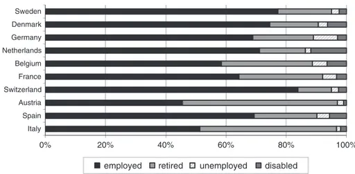
Evidence of unused labour capacity is also available in the SHARE data. Figure 1 shows that very large fractions of individuals aged 50–64 are retired in most coun-tries. A very similar picture can be obtained by focusing on individuals who are fully functioning,2 ruling out a key role of poor health in determining early exits from the labour force. In the figure, and throughout this paper, we focus on heads of household: within couples, we define a person to be the head if he or she is the only one with a work-history, but if both spouses have a work-history the head is taken to be the man.
Figure 1 shows striking differences between neighbouring countries such as Aus-tria and Germany or Switzerland: in AusAus-tria a much larger fraction of individuals are retired. This is in line with the more generous financial incentives for early retirement available in Austria compared to Germany or Switzerland.
0% 20% 40% 60% 80% 100% Italy Spain Austria Switzerland France Belgium Netherlands Germany Denmark Sweden
employed retired unemployed disabled
Figure 1. Economic activity of household heads, aged 50–64
2
An individual is established to be ‘functioning’ on the basis of self-reported health indicators which establish the number of limitations in activities of daily living (ADL) and instrumental activities (IADL). An individual is ‘functioning’ if no limitation is reported.
Figure 1 also shows that an important role is played in some countries by disabil-ity insurance (the Netherlands and Denmark) and unemployment (mostly Germany – former East Germans).
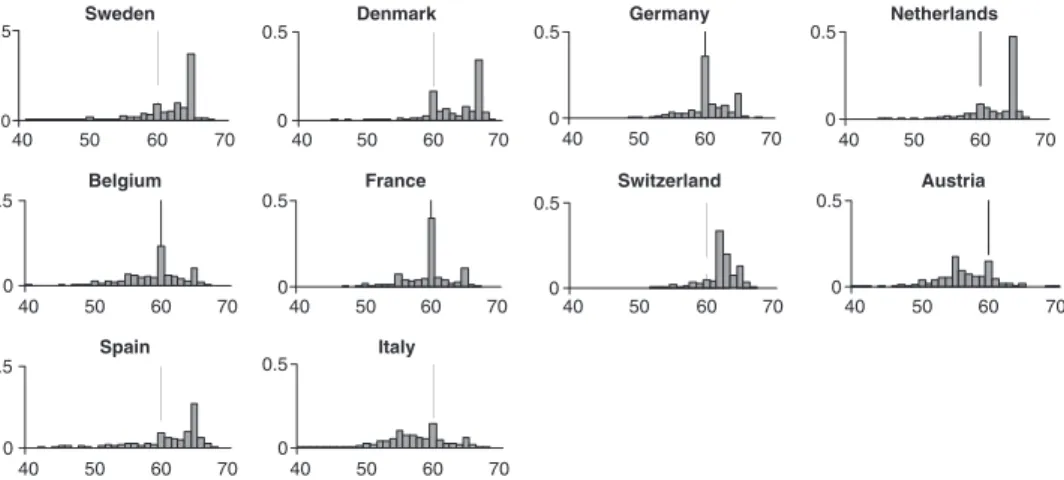
Figure 2 shows histograms of actual retirement age by country – a vertical line marks age 60. Retirement age is based on a recall question asked to the retired. The data refer to heads of households, that is to both men and women, and this explains why the sample densities are often bimodal. The most striking feature is the difference between countries like Sweden and Denmark on the one hand, and Austria and Italy on the other. In the former, few retired before age 60, in the lat-ter most retired aged 60 or less. In the case of the Netherlands the picture is some-what misleading, because respondents on disability insurance were not asked the question, and therefore we do not observe the whole of the left tail of the distribu-tion. This fact (that could apply also to other countries, such as Belgium, Denmark and Spain) should be kept in mind in interpreting the evidence we produce.
One final piece of information that is directly available in SHARE is the propor-tion of currently employed individuals (aged 50 or more) who wish to retire as soon as possible: this ranges from little over 25% in Sweden and Switzerland, to 48% in France, 55% in Italy and 66% in Spain.
These large fractions of working individuals who look forward to retirement sug-gest that job-pension eligibility is an important determinant of the retirement deci-sion. The variability across countries further suggests that differences in economic and institutional incentives play a key role in explaining unused labour capacity.
2.2. Unused financial capacity
The existence of unused financial capacity is less well documented and has attracted less attention in the economic policy debate than unused labour capacity.
France 0 0.5 40 50 60 70 Switzerland 0 0.5 40 50 60 70 Sweden 0 0.5 40 50 60 70 Denmark 0 0.5 40 50 60 70 Germany 0 0.5 40 50 60 70 Netherlands 0 0.5 40 50 60 70 Belgium 0 0.5 40 50 60 70 Austria 0 0.5 40 50 60 70 Spain 0 0.5 40 50 60 70 Italy 0 0.5 40 50 60 70
And yet, differences across European countries in portfolio choice and in home equity release are even more striking.
In practically all countries equity attracts a premium – at least in the long run. Yet, equity holdings are relatively rare in the population at large of all Southern and some Central European countries, as discussed in Guiso et al. (2002). More generally, investment in risky financial assets is limited, and this has the effect of limiting the ability of consumers to enjoy the benefits of growth (increases in pro-ductivity typically lead to higher wages, not necessarily higher pensions) and to hedge macro-wide risks, such as inflation.
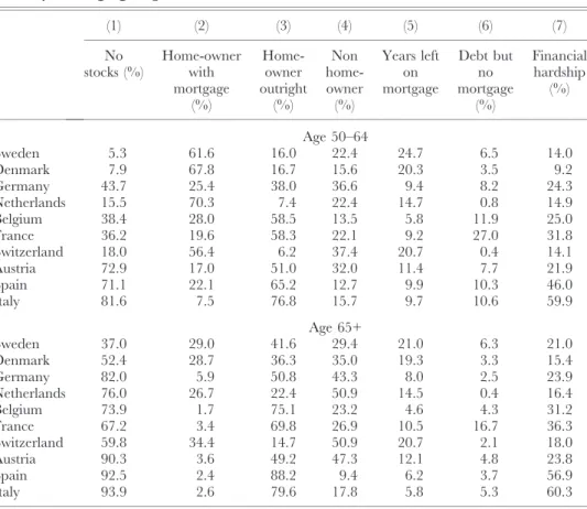
In Table 1 we report descriptive statistics of various indicators of unused finan-cial capacity by country and by age: we split the sample between the younger old (50–64) and the older old (65+).
In column 1 of Table 1 we show the proportions of households who do not hold any stocks (the variable takes value 1 if the household does not hold stocks directly or indirectly, including individual retirement accounts and occupational pensions) by country and age group. We see that equity holdings are much more common in the younger group (50–64) than in the older group (65+) in all countries, and that
Table 1. Indicators of unused financial capacity and financial hardship by country and age group
(1) (2) (3) (4) (5) (6) (7) No stocks (%) Home-owner with mortgage (%) Home-owner outright (%) Non home-owner (%) Years left on mortgage Debt but no mortgage (%) Financial hardship (%) Age 50–64 Sweden 5.3 61.6 16.0 22.4 24.7 6.5 14.0 Denmark 7.9 67.8 16.7 15.6 20.3 3.5 9.2 Germany 43.7 25.4 38.0 36.6 9.4 8.2 24.3 Netherlands 15.5 70.3 7.4 22.4 14.7 0.8 14.9 Belgium 38.4 28.0 58.5 13.5 5.8 11.9 25.0 France 36.2 19.6 58.3 22.1 9.2 27.0 31.8 Switzerland 18.0 56.4 6.2 37.4 20.7 0.4 14.1 Austria 72.9 17.0 51.0 32.0 11.4 7.7 21.9 Spain 71.1 22.1 65.2 12.7 9.9 10.3 46.0 Italy 81.6 7.5 76.8 15.7 9.7 10.6 59.9 Age 65+ Sweden 37.0 29.0 41.6 29.4 21.0 6.3 21.0 Denmark 52.4 28.7 36.3 35.0 19.3 3.3 15.4 Germany 82.0 5.9 50.8 43.3 8.0 2.5 23.9 Netherlands 76.0 26.7 22.4 50.9 14.5 0.4 16.4 Belgium 73.9 1.7 75.1 23.2 4.6 4.3 31.2 France 67.2 3.4 69.8 26.9 10.5 16.7 36.3 Switzerland 59.8 34.4 14.7 50.9 20.7 2.1 18.0 Austria 90.3 3.6 49.2 47.3 12.1 4.8 23.8 Spain 92.5 2.4 88.2 9.4 6.2 3.7 56.9 Italy 93.9 2.6 79.6 17.8 5.8 5.3 60.3
households own stocks much more frequently in Sweden, Denmark, the Nether-lands and Switzerland. In France, Belgium and Germany more than 50% of the younger households have some equity holdings, while in Austria, Italy and Spain participation in the equity markets is much less widespread.
The next three columns provide information on home-ownership. In column (2) we show the fractions of households who own their home but have a mortgage; in column (3) the fractions who own outright. The sum of these two columns provides information on home-ownership overall. Column (4) shows the proportions of households who do not own their home (they may either rent it, or use it for free – either provided by their employer or in usufruct).
We see that home-ownership is relatively high in all countries, with the exception of older households in the Netherlands, Switzerland, Austria and perhaps Germany, where older generations had access to public housing on a mass scale. It is striking to see how high home-ownership is in Southern European countries and in Belgium. It seems that countries where participation in risky financial assets is low are characterized by high home-ownership rates. The question is then whether in these countries households are able to use the equity locked in their homes to sup-port their consumption of non-housing goods and services, or whether instead they are house-rich and cash-poor, as noted for the US by Venti and Wise (2004) and Mitchell and Piggott (2003), and for European countries by Bridges et al. (2006).
The equity locked up in the house can be released in mainly three ways: by either moving from owning to renting, trading down or using the house as collat-eral for secured loans. Selling the home (Chiuri and Jappelli, 2006), and more gen-erally downsizing (Banks et al., 2007) are extreme forms of housing equity withdrawal, that are not widely used in most countries, possibly because of their consumption implications and the high transaction costs involved (both monetary and psychological). Other forms of equity withdrawal do not affect the consumption aspect of housing and do not involve moving costs, but require the use of debt instruments, such as mortgage refinancing (Hurst and Stafford, 2004). Taking up a new mortgage or refinancing an existing mortgage in old age is quite common in some countries, quite rare instead in others.
Column (2) highlights the widespread use of mortgages in some countries: Swe-den, Denmark, the Netherlands and Switzerland, even at older ages. Strikingly, these four countries are the same where households participate most in equity mar-kets. Mortgages in older ages are almost unheard of in all remaining countries, even though non-negligible fractions of mortgagors can be found in the younger age group in Germany, Belgium, France, Austria and Spain.
As we can see from column (5), in Nordic countries, in Switzerland and the Netherlands home-owners often have long-lived mortgages that allow them to keep an adequate standard of living. In these countries the elderly have access to finan-cial instruments (such as reverse mortgages and equity line schemes) that allow them to withdraw equity from the house to finance consumption in old-age.
How-ever, in Mediterranean and some Central European countries mortgages are less often held, particularly by individuals aged 65 or more, and other forms of debt are often resorted to – with widespread self-reported financial hardship.
Column (5) highlights that in those countries where mortgages are common in older ages, they are indeed used to support consumption; that is, households do not necessarily plan to repay them in full while alive. In Denmark, Sweden and Switzerland the average residual life of mortgages is around 20 years for individuals of 65 years of age or more, and in the Netherlands it is around 15 years.
Limited housing equity withdrawal could be due to credit market failures (Bertola et al., 2006), information problems (Jappelli and Pagano, 2006) or financial illiteracy (Christelis et al., 2006; Lusardi and Mitchell, 2007). However, the possibility must be considered that housing equity is used by elderly parents as a means to attract attention by their adult children (Bernheim et al., 1985; Angelini, 2007).
More generally, mortgage refinancing can be used not only to support consump-tion in old age after a negative income or health shock (as stressed by Hurst and Stafford, 2004), but also to rebalance one’s portfolio in response to house price changes (Lusardi and Mitchell, 2007, stress that US baby boomers do this to a rather limited extent). This second use of mortgages requires a certain degree of financial sophistication, and low-cost access to financial markets.3
It is of course possible that homeowners in the remaining countries do not wish to borrow, either for precautionary reasons (to pay for future, uncertain health expenses, say) or because of a strong bequest motive. However, column (6) shows that in at least some cases they use other forms of debt to support their non-housing consumption: in France over 25% of households aged 50–64 who own their home borrow some other way (instalments credit, unsecured loans etc.), and do not take up a mortgage. Non-negligible fractions of homeowners do likewise in Spain, Belgium and Italy, and this may be taken as evidence of either very high transaction costs in the mortgage market or of scarce knowledge of the financial and debt markets by these consumers.
We have seen so far that in some countries the fraction of individuals who partic-ipate in financial markets is relatively small, the fraction of homeowners who have mortgages is also small, and yet there are many who borrow in other forms.
The question is whether in these countries individuals can cope well despite all this, or whether they face financial hardship of some form. The SHARE question-naire contains a useful question on this:
‘Thinking of your household’s total monthly income, would you say that your household is able to make ends meet with great difficulty, with some difficulty, fairly easily or easily?’
3
Lusardi and Mitchell (2007) stress how ‘baby boomers’ in the US rely more on housing equity than other cohorts of indi-viduals: several factors, including the level of financial literacy or the degree of self-commitment, are potentially valid explana-tions of this behaviour, what matters most is that these households might end up being excessively exposed to the risks of house-price bubbles bursts. A similar problem may exist for households in those European countries where portfolios are tilted toward housing wealth.
In column (7) we display the proportions of households who respond that they make ends meet with great or some difficulty. This is particularly high (over 50%) in Spain and Italy, but fractions of 20% or more are found in Belgium, France, Austria and Germany. The lowest fractions are found in Denmark, Switzerland, the Netherlands and Sweden, that is, in the four countries where households appear to make the best use of financial markets and mortgage opportunities. In all other countries we can argue that there is ample unused financial capacity.
A question that naturally arises when dealing with a self-reported indicator of financial distress is to what extent country differences are driven by differences in response styles, and to what extent they instead reflect genuine differences in eco-nomic circumstances. A way to address this issue is to show how average self-reported financial distress correlates to indicators that relate to either consumption or wealth/income.
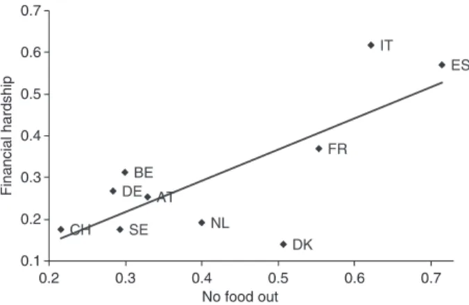
In Figures 3 and 4 we show how the self-reported financial hardship indicator correlates with two indicators based instead on consumption of luxury goods and on availability of liquid assets. In particular, Figure 3 displays the proportion of households in financial hardship against the proportion of households who report never to eat out in a normal month. Eating out is of course partly a matter of taste, partly a matter of relative prices, but in all countries it is a luxury good compared to eating at home – we can expect households in financial distress to eat out less often than households with no financial problems, other things being equal. We see from Figure 3 that there is a strong, positive association between the self-reported indicator of financial hardship and the indicator based on consumption patterns.
Figure 4 shows the relation between the proportion of households in financial hardship and the proportion of households whose liquid assets are less than three times their current monthly income. The latter indicator has been used in the literature on liquidity constraints, following Zeldes (1989) – for older households
IT ES FR DK NL AT DE BE SE CH 0.1 0.2 0.3 0.4 0.5 0.6 0.7 0.2 0.3 0.4 0.5 0.6 0.7 No food out Financial hardship
Figure 3. Proportion of households in financial hardship against the propor-tion of households who report never to eat out
this indicator likely captures lack or inability to make the best use of illiquid wealth. Here again, we observe that there is a strong, positive correlation between the self-reported measure and this more conventional indicator of finan-cial hardship.
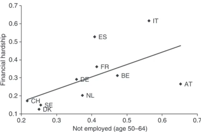
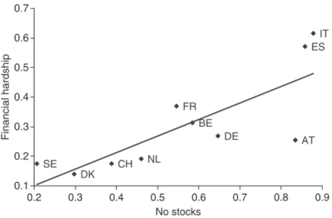
The issue we are going to investigate in what follows is whether and to what extent financial hardship is related to both unused labour capacity and unused financial capacity. A graphical analysis shows that there is prima facie evidence for both relations. In Figure 5 we display the proportion of households in financial hardship against the proportion of individuals aged 50–64 who do not work. In Figure 6 we display the proportion of households in financial hardship against the proportion of households with no stocks in their portfolios. In both cases we see that there is a positive association. IT CH SE BE DE AT NL DK FR ES 0.1 0.2 0.3 0.4 0.5
Financial wealth < 3 months of income 0.1 0.2 0.3 0.4 0.5 0.6 0.7 Financial hardship
Figure 4. Proportion of households in financial hardship against the propor-tion of households whose financial wealth is less than three times their monthly income CH SE BE DE AT NL DK FR ES IT 0.2 0.3 0.4 0.5 0.6 0.7
Not employed (age 50–64) 0.1 0.2 0.3 0.4 0.5 0.6 0.7 Financial hardship
Figure 5. Proportion of households in financial hardship against the propor-tion of households who do not work
2.3. The early retirement trap
We have shown above that different fractions of individuals are retired in their late fifties/early sixties in different European countries – something known in the litera-ture as unused labour capacity – and argued that these differences may be the response to early retirement incentives, as stressed in Gruber and Wise (1999, 2004). We have also shown that different fractions of individuals fail to make cor-rect use of financial and debt markets – something we labelled unused financial capacity – and that in those countries where unused financial capacity is more com-mon, larger fractions of individuals face financial hardship. The question we are going to address in this section is whether and to what extent unused labour and financial capacity interact in generating financial hardship.
We present in Box 1 a model where individuals are induced to retire early by a gen-erous early retirement scheme in the public pension system, but find themselves in financial hardship later because of negative shocks. A key element of this model is that financial and insurance markets are incomplete: in these circumstances postponing retirement would be a way for consumers to partially insure against negative shocks (as argued in Bodie et al., 1992). The early retirement financial incentive is strong enough to make early retirement optimal ex ante, even though ex post large fractions of consumers may regret foregoing the insurance opportunities entailed by continued work. In a world of incomplete markets (limited access to the financial markets, no or inadequate health and long-term care insurance policies for elderly individuals), this may prove ex post sub-optimal for those who have indeed been hit by adverse shocks.
We know that the welfare state is quite different across European countries: in some Southern and Central European countries, the state gives generous pension benefits to early retirees, in Northern and some other Central European countries instead public pension benefits are lower, but the public health system provides both acute and long-term care, and tax incentives are used to induce individuals to contribute to occupational and private pensions (that invest in equity) and to purchase private health insurance.
IT ES FR DK NL AT DE BE SE CH 0.2 0.3 0.4 0.5 0.6 0.7 0.8 0.9 No stocks 0.1 0.2 0.3 0.4 0.5 0.6 0.7 Financial hardship
Figure 6. Proportion of households in financial hardship against the propor-tion of individuals aged 50–64 who do not own stocks
Box 1. The model
To be more precise on how early retirement can be a trap for forward-look-ing consumers, we present a 3-period model with incomplete markets: all individuals work in period 0 and are retired in period 2, but must decide whether to retire in period 1 or continue working before finding out whether they are going to be affected by (costly) health problems in period 2. If they retire, they enjoy leisure and receive a pension bE in both periods 1 and 2; if they work in period 1 they can choose hours of work (T ) ‘1), and receive labour income w(T ) ‘1). Their pension in period 2 will then be bL.
Formally, individuals maximize an expected utility index in two steps: first, they choose period 0 consumption (C0) and decide whether to take early (E) or late (L) retirement. Next, they observe the health shock realiza-tion that will affect them in period 2. If they have chosen to retire early, they decide how much consumption to allocate to periods 1 and 2 (C1, C2); if instead they have chosen to retire late, they also decide how much leisure (‘1) to enjoy in period 1.
Expected life-time utility is: UðC0; ‘0Þ þ 1 1 þ dmaxE;‘ E $ UðC1L; ‘1Þ þ 1 1 þ dUðC L 2; TÞ ! " ; UðC1E; TÞ þ 1 1 þ dUðC E 2; TÞ ! " # $
where d is their time preference parameter.
This is maximized subject to the following constraints: A1L¼ ð1 þ r ÞðY0& C0LÞ
Y0' wðT & ‘0Þ AL1 þ wðT & ‘1Þ ¼ C1Lþ sL1
bLþ s1Lð1 þ r Þ & x ¼ C2L if they work in period 1, and
A1E ¼ ð1 þ r ÞðY0& C0EÞ Y0' wðT & ‘0Þ A1Eþ bE ¼ C1Eþ s1E bE þ s1Eð1 þ rÞ & x ¼ C2E
if instead they opt for early retirement. In the above, A1 denotes assets that are carried over from the previous period, s1is period 1 saving and x is the shock that takes value F with probability p, 0 with probability (1 – p).
We further assume bE< bL, and consider the cases where early retire-ment is actuarially fair
bEþ bE 1 þ r ¼
bL 1 þ r
or, instead, early retirement is made financially attractive: bEþ
bE 1 þ r>
bL 1 þ r:
In this model the decision to work in period 1 implies foregone leisure and foregone pension bE, but allows consumers to change hours if adverse shocks occur. Depending on the relative size of bE and bL, consumers may choose to retire early, but find out later that they are in financial hardship because of the shocks.
We solve the model for the case where utility takes the following form: UðC; ‘Þ ' lnðCÞ þ a lnð‘Þ:
In this model, early retirement is never chosen in the actuarially fair case. In fact, consumers can receive the same pension in present value terms whether they retire in period 1 or in period 2, but can work in period 1 only if they retire in period 2. Early retirement is weakly dominated, because it imposes an extra constraint on an otherwise identical optimiza-tion problem.
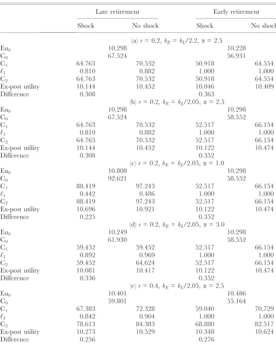
Depending on the taste for leisure, early retirement can be made attrac-tive ex-ante if its benefits are sufficiently large. In the calibrations of the model we set period 0 labour income, Y0, equal to 100, the hourly wage equal to 200 and we normalize T to 1. The shock variable, x, is taken to be 0.3Y0 with probability p = 0.5 and 0 otherwise. In the first case we analyse, we assume the interest rate and the time preference parameter d to be 0.2, we set a = 2.5 and make the late retirement benefits, bL, equal to 80% of period 0 labour income, Y0. When early retirement is actuarially fair (see panel a in Table 2), the late retirement option dominates the early retire-ment option both in terms of ex-ante expected utility, and in terms of ex-post variability in realized utility for the two possible outcomes of the shock (real-ized utility is defined as life-time utility corresponding to the optimal values of consumption and leisure, and the realized value of the shock variable, x. Its variability is simply the difference between realized utility in the two cases). We find that the consumer becomes indifferent ex-ante between early
and late retirement if early retirement benefits are increased in such a way that (for the given value of bL = 0.8Y0)
bE þ bE 1:05¼
bL 1:05:
In this case, ex-post life-time utility is more disperse where the consumer opts for early retirement (as shown in panel b, utility ranges between 10.474 in the zero shock case to 10.122 when the shock hits if the consumer retires early; from 10.452 to 10.144 in the late retirement case).
When consumers have less taste for leisure, they opt for late retirement (as shown in Table 2 for a = 1, see panel c). Consumers who enjoy leisure more will instead take early retirement, even though they face low utility when the shock hits (as shown in Table 2 for a = 3, panel d). Of course, the choices made in the case of early retirement are unaffected by changes ina, as shown in the last two columns of panels b, c and d.
Thus financially advantageous early retirement schemes lead to financial hardship (low ex-post utility) for consumers hit by negative shocks. This hap-pens despite the presence of precautionary savings in period 0, and of fur-ther savings in period 1, simply because early retirees can no longer forego leisure in period 1 to buffer the (by then) perfectly foreseen period 2 shock. This situation can be taken to represent what happens (or used to happen until a few years ago) in some Mediterranean and Central European coun-tries.
In this model a first best solution can be achieved if a fair health insur-ance scheme is introduced. The health shock we consider is best interpreted as generating long-term care needs, that are typically well covered by the government or private insurance schemes in Nordic and some Central Euro-pean countries. In Southern EuroEuro-pean countries instead long-term care is inadequately covered by the government, while private insurance policies are not available for this type of health risk (Callegaro and Pasini, 2008). To appraise the quantitative importance of long-term care, we can point to just one indicator: in Sweden and the Netherlands almost 9% of 65+ individu-als are in institutional care; this proportion is less than 4% in Italy and Spain (see Table 2 in Bolin et al., 2008, for further details).
In the model consumers can only use one, low-return financial asset (if periods are 20-year long, a 20% real return is what is normally obtained by investing in short-term government debt or in saving accounts). Modelling the availability of further financial assets is beyond the scope of this paper (Bodie et al., 1992, analyse the household life-time portfolio choice when stocks are risky; they show that flexibility in leisure choice is associated to higher demand for stocks – in their model, leisure is used to insure the risk
of low stock returns), but we can check what the consequences would be if a higher-return asset was made available. We do this in panel e of Table 2, where the interest rate is increased to 0.4, while the time preference param-eter and early retirement pension benefits are as in the previous panels. We can think of this as a case where stocks are made easily available to house-holds. This has a positive wealth effect and therefore it makes early retire-ment more attractive, because leisure is a normal good – we know that this would not be the case if stock returns were risky (see Bodie et al., 1992). However, given that early retirement is chosen, we see that stocks help reduce the spread between ex-post utilities (the difference between realized utilities with early retirement is just 0.276 compared to 0.352 of panel b – a larger reduction, 0.076, than for late retirees, 0.052), that is, the availability of a high-yielding asset reduces financial hardship for early retirees.
We argue that individuals who live in the first group of countries may find that early retirement is a trap: it is financially advantageous ex ante, but shuts down the possibility to buffer adverse shocks by increasing labour supply ex post. In the model we present, individuals decide in their middle age whether to take early retirement or not, and then find out if they are going to require long-term care in old age. Other individual-specific shocks that would fit this framework are illness/disability of a parent or the spouse at any time after the retirement decision is taken. A more complex model would also contemplate economy-wide shocks, such as inflation on goods that are particularly important for the elderly (such as medical goods and ser-vices, or heating fuel, see Miniaci et al., 2008), that may be hedged by investment in equity.
The question remains of why, in economies where financial and insurance mar-kets do not operate well, pensions are typically more generous. A possible reason is that in countries with incomplete markets governments have opted for paying higher benefits to the retirees, in order to encourage informal risk-sharing arrange-ments (Lindbeck and Persson, 2003).
It is worth stressing that early retirement as intended in the model does not nece-ssarily match national definitions. Variability in the access to early retirement bene-fits (and to old age benebene-fits) is marked both across European countries and, within each country, across types of employment and years. For example, in Italy the stat-utory retirement age for women was 55 until recently and is now 60 (like in Aus-tria), while in Sweden the old-age retirement age was 67 for a long time for both men and women (it changed to 65 in 1995): Appendix B provides a summary of these features for the relevant SHARE countries. Some countries had explicit early retirement schemes only in some periods, while others allowed and still allow for early retirement at very early ages (Italy). This variability in institutional set-ups is
quite striking from the point of view of participation to the labour force which we explore in this paper, as it turns out that in some countries the statutory retirement age is (or was) so low that it is below the early retirement age in other countries, hence making the concept of ‘early retirement’ hard to define in a clear and consistent way.
What matters for this model is whether individuals are retired for a shorter or longer period. This reflects preference heterogeneity (taste for leisure), differences in
Table 2. Numerical solutions of the theoretical model
Late retirement Early retirement
Shock No shock Shock No shock
(a) r = 0.2, bE= bL/2.2,a = 2.5 Eu0 10.298 10.228 C0 67.524 56.931 C1 64.763 70.532 50.918 64.554 ‘1 0.810 0.882 1.000 1.000 C2 64.763 70.532 50.918 64.554 Ex-post utility 10.144 10.452 10.046 10.409 Difference 0.308 0.363 (b) r = 0.2, bE= bL/2.05,a = 2.5 Eu0 10.298 10.298 C0 67.524 58.552 C1 64.763 70.532 52.517 66.154 ‘1 0.810 0.882 1.000 1.000 C2 64.763 70.532 52.517 66.154 Ex-post utility 10.144 10.452 10.122 10.474 Difference 0.308 0.352 (c) r = 0.2, bE= bL/2.05,a = 1.0 Eu0 10.808 10.298 C0 92.621 58.552 C1 88.419 97.243 52.517 66.154 ‘1 0.442 0.486 1.000 1.000 C2 88.419 97.243 52.517 66.154 Ex-post utility 10.696 10.921 10.122 10.474 Difference 0.225 0.352 (d) r = 0.2, bE= bL/2.05,a = 3.0 Eu0 10.249 10.298 C0 61.930 58.552 C1 59.452 59.452 52.517 66.154 ‘1 0.892 0.969 1.000 1.000 C2 59.452 64.624 52.517 66.154 Ex-post utility 10.081 10.417 10.122 10.474 Difference 0.336 0.352 (e) r = 0.4, bE= bL/2.05,a = 2.5 Eu0 10.401 10.486 C0 59.801 55.164 C1 67.383 72.328 59.040 70.729 ‘1 0.842 0.904 1.000 1.000 C2 78.613 84.383 68.880 82.517 Ex-post utility 10.273 10.529 10.348 10.624 Difference 0.256 0.276
life-time resources (the worse off cannot afford to retire early), as well as the implicit tax rate of postponing retirement – as emphasized by Gruber and Wise (1999). In estimation, we want to capture this last effect – to this end, we shall instrument years into retirement with years into eligibility (as suggested in Battistin et al., 2008, in their analysis of the retirement consumption drop in Italy). We shall come back to this point when we describe our identification strategy.
To summarize, our model can be seen to predict the following:
a) where early retirement is made attractive and financial markets do not work well, individuals who retire early are better off in the short run, but worse off in the long run (that is: an increasing fraction of them will face financial hard-ship) – this should be the case of countries like Italy and Austria;
b) where financial markets work well, and early retirement is not made attractive, when people retire should not matter to their financial situation later in life – this should be the case of countries like Denmark and Sweden;
c) in general, failure to use financial markets should increase the risk of facing finan-cial hardship – also, the longer individuals have been retired for a given age, the more likely they face financial hardship unless they can fully insure all risks.
3. EMPIRICAL SPECIFICATION AND ESTIMATION RESULTS
The Survey of Health, Ageing and Retirement in Europe (SHARE) is a unique multidisciplinary and cross-national dataset that contains a large amount of information on the physical and mental health, economic and social capital of individuals aged 50 and over, and follows them over time (for an appraisal, see Bo¨rsch-Supan et al., 2005, 2008).
The SHARE data are well suited both to provide fresh evidence on the issues highlighted above across a host of European countries (11 in the 2004 wave, 15 in the 2006–7 wave), and to relate the observed pattern of unused labour capacity to the financial situation of the early retirees, controlling for the role played by social and family relations, as well as by welfare regimes. The evidence we present here is based on an early release version of wave 2 SHARE data, and covers 10 countries for which we could construct the required retirement eligibility variables (these are the countries shown in all previous figures).
The aim of this paper is to shed light on the ‘early retirement trap’: the empirical specification requires modelling the way financial hardship depends on unused financial capacity and unused labour capacity, and how these two interact.
The SHARE survey contains a question that can be used to assess financial hard-ship: a qualitative indicator of difficulty making ends meet. We treat households who report difficulties as in financial hardship (or distress).
We construct indicators of unused financial capacity in two dimensions: limited diver-sification across asset types (households are not well diversified, no stocks, if they do not hold stocks directly or indirectly, including individual retirement accounts and
occupational pensions), and failure to tap in home equity (for those homeowners who have debts but no mortgage, debt but no mortgage). The former indicator is defined for all households, the latter only for homeowners. We also construct indi-cators of unused labour capacity, in the form of years elapsed from the retirement (for retired people) and years to retirement (for workers) (years from retirement, years to retire-ment). Given that we control for age, individuals with more years from retirement are those who left the labour market earlier.
Our estimation strategy is the following: we estimate financial hardship equa-tions, where the dependent variable takes the value 1 if the household reports some or great difficulties making ends meet, zero otherwise (financial hardship), as a func-tion of a number of household and individual characteristics as well as variables that capture household wealth, unused labour and financial capacity indicators. The starting sample consists of all households who are either working or retired (hence excluding other households out of work) in Denmark, Belgium, France, Aus-tria, Spain, Italy, the Netherlands, Sweden, Switzerland and Germany for a total of 11,496 observations. When we use the variable debt but no mortgage, we select home-owners, and our sample is reduced to 8,313 observations.4
Throughout our analysis we condition on a set of explanatory variables, that includes characteristics of the head (age and its square, sex, years of education, self-reported health, mobility problems, fluency and recall ability), plus house-hold-level variables (household size, and a couple dummy) and a set of country dummies.
In the financial hardship equation, we also control for a few economic variables – which we treat as potentially endogenous in estimation. These include wealth (the sum of financial wealth and real wealth, net of debt and mortgages) and household social security wealth. An individual’s social security wealth is the discounted value of future benefits expected by the individual given the current legislation and given longevity (for further details see Appendix B).
Our identification strategy rests on the following assumptions: we assume that risk aversion and financial literacy are instruments for the unused financial capacity indicators (no stocks, and debt but no mortgage where applicable). We take the number of rooms in the main residence as an instrument for wealth (that is, the sum of financial and real assets, net of liabilities), on the assumption that the main residence is cho-sen earlier in life and is not easily changed in response to shocks. Retirement status of the head (retired) is instrumented by a job-pension eligibility variable that we con-struct by taking into account country-specific early retirement legislation by occupa-tion, gender, year of retirement and potential years of contributions. Similarly, years from/to retirement are instrumented by years to/from eligibility (job-pension eligibility is further described in Appendix B, where it is shown how and to what
4
We classify individuals by their employment status as either employed (either employee or self-employed) or retired (that includes all those who report themselves as retired from work, but for those who currently do some paid work).
extent eligibility varies within countries). Household social security wealth, that is based on actual or expected retirement age, is instrumented by a potential social security wealth variable, that is based on legal retirement age (further details on how these two variables were calculated are also provided in Appendix A). Institutional differ-ences across countries and groups of individuals are thus exploited to construct a set of instruments for retirement-related explanatory variables, following the sugges-tions made by the unused labour capacity literature discussed above.
Given that financial hardship is a dichotomous variable, and so also are the unused financial capacity indicators, taking into account the endogeneity of these indicators requires estimating a seemingly unrelated system of probit equations for financial hardship, no stocks and debt but no mortgage, where the last two equations include as additional instruments indicators of risk aversion (low risk aversion and med-ium risk aversion) of likely proximity to banks (rural), and of financial literacy (this is summarized in the ability to calculate percentages, percentage calculation, to divide a number by a ratio, lottery division, and to calculate compound interest rates, compound interest). The wealth and unused labour capacity variables that enter the first equation are also potentially endogenous, but continuous, and instrumental variables estimates can be computed by adding to the equation the residuals from the first stage.
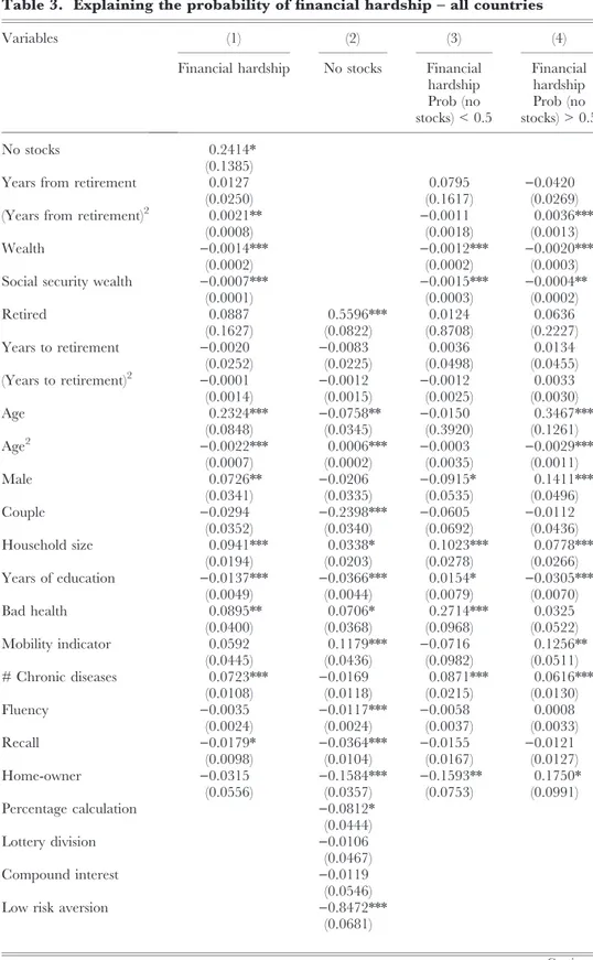
In Table 3 we present estimation results for the whole sample that includes homeowners and tenants. Therefore, the only indicator of unused financial capacity is no stocks. In column (1) we show how the probability of financial hardship is affected by not having stocks for all households (no stocks) and by the number of years elapsed since retirement (years from retirement), controlling for age and demo-graphic variables, but also for economic variables that relate to wealth. Our theoretical model predicts that risky assets should lower the probability of financial hardship, while years from retirement should increase it (at least after a sufficiently long time interval, if early retirement is financially advantageous).
In estimation, years from retirement (and its square), wealth and social security wealth are treated as endogenous and instrumented, by adding the first stage resid-ual to the regression. Also treated as endogenous is the no stocks dummy variable – this is jointly estimated in a bivariate probit system (parameter estimates are reported in column 2). Other variables (years to retirement and its square, and retired) are instead treated as exogenous, following the results of a Hausman test (see column 1 in Table A1 of the Appendix).5
5
The inclusion of several binary endogenous variables in probit-style equations leads to non-trivial computational problems, but a Hausman-style test is easily conducted by introducing in the regression the residuals from the first stage equations for all possibly endogenous variables (see for instance Wooldridge, 2002, pp. 472–8), whether discrete or continuous. In our case, these first stage regressions are all well determined – the only feature worth reporting is that wealth is heavily affected both by number of rooms in the main residence and by the risk aversion indicators, and the latter play a key role in explaining the probability of having risky assets. The probability of not having stocks is also explained by financial literacy, but the com-mon dependency of wealth and no stocks on the risk aversion indicators results in less precise estimates of the coefficient of the latter variable in the financial hardship equation.
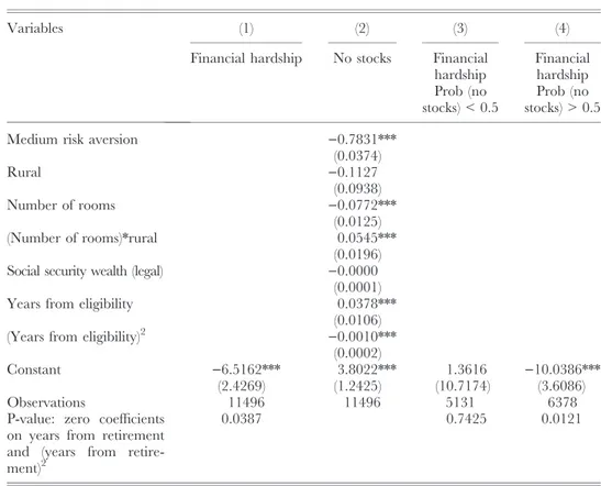
Table 3. Explaining the probability of financial hardship – all countries
Variables (1) (2) (3) (4)
Financial hardship No stocks Financial hardship Prob (no stocks) < 0.5 Financial hardship Prob (no stocks) > 0.5 No stocks 0.2414* (0.1385)
Years from retirement 0.0127 0.0795 )0.0420
(0.0250) (0.1617) (0.0269)
(Years from retirement)2 0.0021** )0.0011 0.0036***
(0.0008) (0.0018) (0.0013)
Wealth )0.0014*** )0.0012*** )0.0020***
(0.0002) (0.0002) (0.0003)
Social security wealth )0.0007*** )0.0015*** )0.0004**
(0.0001) (0.0003) (0.0002) Retired 0.0887 0.5596*** 0.0124 0.0636 (0.1627) (0.0822) (0.8708) (0.2227) Years to retirement )0.0020 )0.0083 0.0036 0.0134 (0.0252) (0.0225) (0.0498) (0.0455) (Years to retirement)2 )0.0001 )0.0012 )0.0012 0.0033 (0.0014) (0.0015) (0.0025) (0.0030) Age 0.2324*** )0.0758** )0.0150 0.3467*** (0.0848) (0.0345) (0.3920) (0.1261) Age2 )0.0022*** 0.0006*** )0.0003 )0.0029*** (0.0007) (0.0002) (0.0035) (0.0011) Male 0.0726** )0.0206 )0.0915* 0.1411*** (0.0341) (0.0335) (0.0535) (0.0496) Couple )0.0294 )0.2398*** )0.0605 )0.0112 (0.0352) (0.0340) (0.0692) (0.0436) Household size 0.0941*** 0.0338* 0.1023*** 0.0778*** (0.0194) (0.0203) (0.0278) (0.0266) Years of education )0.0137*** )0.0366*** 0.0154* )0.0305*** (0.0049) (0.0044) (0.0079) (0.0070) Bad health 0.0895** 0.0706* 0.2714*** 0.0325 (0.0400) (0.0368) (0.0968) (0.0522) Mobility indicator 0.0592 0.1179*** )0.0716 0.1256** (0.0445) (0.0436) (0.0982) (0.0511) # Chronic diseases 0.0723*** )0.0169 0.0871*** 0.0616*** (0.0108) (0.0118) (0.0215) (0.0130) Fluency )0.0035 )0.0117*** )0.0058 0.0008 (0.0024) (0.0024) (0.0037) (0.0033) Recall )0.0179* )0.0364*** )0.0155 )0.0121 (0.0098) (0.0104) (0.0167) (0.0127) Home-owner )0.0315 )0.1584*** )0.1593** 0.1750* (0.0556) (0.0357) (0.0753) (0.0991) Percentage calculation )0.0812* (0.0444) Lottery division )0.0106 (0.0467) Compound interest )0.0119 (0.0546)
Low risk aversion )0.8472***
(0.0681)
Several demographic explanatory variables have significant coefficients in column (1), most notably education of head, age, health and mobility problems indicators. Country dummies also have significant coefficients, that we shall discuss later (see Table 4). Among the economic variables, wealth and social security wealth have strong, negative effects; years from retirement has a positive, jointly significant effect, whereas no stocks has a positive, but only marginally significant, impact on the prob-ability of financial hardship. The first stage regression for no stocks produces signifi-cant coefficients on many covariates that also affect financial hardship, but also on the risk aversion variables. Notably, financial literacy variables play little role in this equation.
These estimates show that the failure to diversify the portfolio does increase the probability of financial hardship, as expected. They also show that financial hard-ship is more likely if the head is retired compared to employed.
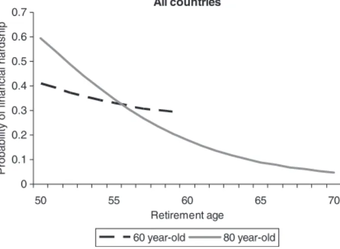
We can work out the implications of our point estimates by computing the mar-ginal effects on the hardship probability of years from retirement for a given age. In Figure 7 we present the marginal effects for a male, living in a couple, retired – the other variables are at their means at ages 60 and age 80.
Table 3. Continued
Variables (1) (2) (3) (4)
Financial hardship No stocks Financial hardship Prob (no stocks) < 0.5 Financial hardship Prob (no stocks) > 0.5
Medium risk aversion )0.7831***
(0.0374) Rural )0.1127 (0.0938) Number of rooms )0.0772*** (0.0125) (Number of rooms)*rural 0.0545*** (0.0196)
Social security wealth (legal) )0.0000
(0.0001)
Years from eligibility 0.0378***
(0.0106)
(Years from eligibility)2 )0.0010***
(0.0002)
Constant )6.5162*** 3.8022*** 1.3616 )10.0386***
(2.4269) (1.2425) (10.7174) (3.6086)
Observations 11496 11496 5131 6378
P-value: zero coefficients on years from retirement and (years from retire-ment)2
0.0387 0.7425 0.0121
Note: Standard errors in parentheses (***p < 0.01, **p < 0.05, *p < 0.1). All specifications include a set of country dummies.
The solid line represents the probability of financial hardship for someone who is today 80 years of age as a function of their age of retirement (long-run effect). It is computed for a male living in a couple and at the sample means of all other explanatory variables in Table 3, using point estimates of all parameters. This
func-All countries 50 55 60 65 70 Retirement age 60 year-old 80 year-old 0.1 0 0.2 0.3 0.4 0.5 0.6 0.7
Probability of financial hardship
Figure 7. Marginal effects of retirement age on financial hardship – all countries
Table 4. Country effects on financial hardship in different specifications
Coefficient No controls Standard set of controls Unused capacity controls
(1) (2) (3) Denmark 0.1212 0.1089 0.1712 (0.0088) (0.0089) (0.0231) Belgium 0.2847 0.3027 0.2641 (0.0118) (0.0133) (0.0165) France 0.3432 0.3869 0.3603 (0.0127) (0.0149) (0.0169) Austria 0.2316 0.1528 0.0836 (0.0157) (0.0134) (0.0182) Spain 0.5210 0.4952 0.4197 (0.0184) (0.0213) (0.0308) Italy 0.6017 0.5107 0.3593 (0.0140) (0.0172) (0.0411) Netherlands 0.1562 0.1306 0.1655 (0.0106) (0.0100) (0.0172) Sweden 0.1763 0.1390 0.2150 (0.0100) (0.0096) (0.0251) Switzerland 0.1594 0.2166 0.2476 (0.0127) (0.0178) (0.0228) Germany 0.2408 0.1739 0.1699 (0.0125) (0.0120) (0.0129) Mean 0.2836 0.2617 0.2456 Variance 0.0263 0.0234 0.0113
tion decreases with retirement age: the longer a person of that generation has been retired, the more likely that person is in financial hardship. For this generation, early retirement increases the probability of current financial hardship. The dashed line shows the same probability for someone who is currently 60 years of age (short-run effect). Also for this group, retiring at young ages increases the probabil-ity of financial hardship, but the curve is less steep: early retirement is less harmful in the short run than in the long run. The relative position of the two lines is not necessarily meaningful, because they refer to different generations.
We can also split the sample according to the probability of having stocks: column 3 presents estimates for the 5,131 households whose estimated probability of owning stocks is greater than half, column 4 refers instead to the other half of the sample (6,378), who are more at risk of suffering as a result of early retirement. As expected, the effects of years from retirement are much stronger for individuals belonging to this latter group (the p-value of the joint test is reported at the bottom of the table), even though the sign of the linear coefficient turns negative, implying that early retirement is good in the short run. The strongly positive coefficient on the squared term implies that early retirement has bad effects in the long run, that is, it eventually increases the probability of financial hardship.
An interesting exercise is to look at how far cross-country differences in financial hardship can be explained by unused financial and labour capacity. To this end we present in Table 4 the probabilities implied by estimated parameters of country dummies for three different specifications: in column (1) there are absolutely no controls in the probit equation (so the estimates predict the average probabilities), in column (2) all the demographic and economic controls used in Table 3 are in the specification, but for the financial capacity (no stocks) and labour capacity (retire-ment, years from retire(retire-ment, years to retirement) variables. Column (3) instead corresponds to column (1) of Table 3. Unlike Table 3, there is no baseline country – all other explanatory variables are expressed in deviations from their sample means.
A comparison between columns (1) and (2) suggests that in some countries house-hold size and composition, age, health, education and wealth make little difference to the average probability of financial hardship. Overall, the average of the country effects is slightly smaller, but their variance is almost identical.
A much clearer picture emerges from comparing columns (2) and (3): adding financial and labour capacity variables further reduces average effects, but much more importantly more than halves their variance. This implies that unused finan-cial and labour capacity indicators play a key role in explaining why finanfinan-cial hard-ship differs so much across European countries, as shown in column (7) of Table 1.
The remarkable decrease in the variability of country dummy coefficients when unused capacity indicators are introduced in the regressions strongly supports the importance of these factors in explaining financial hardship patterns across countries. However, the fact that some variability remains is worth noticing. This may simply reflect differences in reporting styles, with individuals in Latin countries being more
prone to report difficulties compared to individuals in Sweden, Denmark, Germany and the Netherlands. Also, some differences may indeed relate to the noted lack of long-term care coverage in Southern European countries – a factor that is only partly captured by the unused financial capacity proxies used in our regression.
We have run some robustness checks on the basic specification reported in Table 3. First of all, we considered the possibility that wealth does not fully capture the role of precautionary savings – and therefore allowed risk aversion to have a direct impact on financial hardship. While the coefficient for medium risk-aversion was significant, the pattern of estimated coefficients did not conform to expecta-tions, and the coefficients on the key unused labour capacity variables were qualita-tively unaffected. Also, we tried to use financial literacy variables as an indicator of unused financial capacity, rather than the no stock indicator. Again, the unused labour capacity coefficients were unaffected. Estimated financial literacy coefficients suggested that all relevant variability lies in the first indicator (percentage calculation), that was marginally significant in the financial hardship equation, but splitting the sample according to it did not produce significantly different coefficients on the variables of interest.
Overall, we can interpret the estimates shown in Tables 3 and 4 as evidence that both unused financial capacity and unused labour capacity contribute to financial hardship. These estimates support the claim that early retirement can be a trap: workers who were induced to take early retirement by the financial incentives built into the public pensions systems are now more likely to find themselves in financial hardship.
In Table 5 we present estimates of financial hardship probabilities for the sub-sample of home-owners, as this allows us to add the other financial capacity indica-tor to the system of equations, that is, the presence of unsecured debt without a mortgage. As stressed above, this likely indicates that households pay more interest than necessary, and may either point to their financial illiteracy or to high transac-tion costs on mortgages. In this exercise, we treat as endogenous the same variables as in Table 3 (Hausman test results are reported in Table A1), plus of course the debt but no mortgage indicator.
We see that both indicators of unused financial capacity have strong effects on financial hardship, with the predicted signs – the quadratic polynomial in years from retirement also has jointly highly significant coefficients (the p-value of the F-test is less than 1%), but qualitatively similar to those shown in Table 3.
The theoretical model sketched in Section 2.3 suggests that in some countries early retirement should be advantageous in the short run, but detrimental in the long run – these are the countries that allow individuals to retire early (in their fifties) without a suitable reduction in their retirement income. In some other countries, instead, early retirement is actuarially neutral, or even not allowed at all (in which case, other forms of income support are in place for those individuals who lose their jobs in their fifties, or are hit by adverse health shocks that limit their working ability).
Table 5. Explaining the probability of financial hardship for homeowners – all countries
Variables (1) (2) (3)
Financial hardship No stocks Debt but no mortgage
No stocks 0.3793***
(0.0661)
Debt but no mortgage 0.3643***
(0.1177)
Years from retirement 0.0355
(0.0282) (Years from retirement)2 0.0038***
(0.0013)
Wealth )0.0010***
(0.0001)
Social security wealth )0.0009***
(0.0001) Retired )0.1176 0.5454*** 0.1016 (0.1851) (0.0961) (0.1156) Years to retirement 0.0003 )0.0079 )0.0162 (0.0300) (0.0263) (0.0318) (Years to retirement)2 )0.0004 )0.0006 )0.0017 (0.0018) (0.0017) (0.0021) Age 0.4455*** )0.0431 0.0412 (0.1288) (0.0421) (0.0525) Age2 )0.0040*** 0.0004 )0.0005 (0.0011) (0.0003) (0.0004) Male 0.1058*** )0.0509 0.0799 (0.0410) (0.0396) (0.0514) Couple 0.0227 )0.2687*** 0.0251 (0.0411) (0.0392) (0.0507) Household size 0.1052*** 0.0508** 0.0574** (0.0223) (0.0235) (0.0278) Years of education )0.0187*** )0.0397*** )0.0077 (0.0058) (0.0051) (0.0069) Bad health 0.0494 0.0620 )0.0362 (0.0513) (0.0446) (0.0581) Mobility indicator 0.0222 0.0663 0.0246 (0.0624) (0.0533) (0.0684) # Chronic diseases 0.0604*** )0.0106 0.0551*** (0.0135) (0.0144) (0.0182) Fluency )0.0050* )0.0109*** 0.0106*** (0.0029) (0.0028) (0.0036) Recall )0.0021 )0.0364*** )0.0109 (0.0121) (0.0122) (0.0159) Percentage calculation )0.1082** )0.0153 (0.0543) (0.0670) Lottery division )0.0323 )0.1023 (0.0563) (0.0723) Compound interest )0.0247 )0.1629* (0.0650) (0.0868)
Low risk aversion )0.9003*** )0.0454
(0.0793) (0.0883)
Medium risk aversion )0.7758*** )0.0285
(0.0425) (0.0583)
It therefore makes sense to estimate separate financial hardship equations for groups of countries that are relatively homogenous in the way they treat early retirees. Small sample sizes unfortunately prevent us from estimating these equations country by country.
In what follows, we split the sample between generous early retirement countries and ‘actuarially fair’ countries. Belgium, France and Italy were found to be ‘generous’ in Gruber and Wise (1999) – Austria was not considered in that study, but Blo¨ndal and Scarpetta (1998) show its early retirement provisions to be quite similar. Denmark, Sweden and Switzerland do not favour early retirement accord-ing to Gruber and Wise (1999), and we therefore classify them together. We do not include the Netherlands among the group of more generous countries, despite the large number of individuals who take up disability insurance as a pathway to retire-ment, because we are forced to exclude from the analysis precisely those individu-als, for whom we cannot compute the key unused labour capacity variables (years from retirement and years from eligibility variables).
In column (1) of Table 6 we report estimates of financial hardship (and not having stocks) equations for the former group of countries, in column (3) we do likewise for the latter group. Notably, we find that the key estimated coefficients on the years from retirement quadratic polynomial are highly significant in Austria, Belgium, France and Italy, while they are not at all significant in Denmark, Sweden and Switzerland. The coefficient on no stocks has a positive sign in both cases, but in both cases it is also insignificant. This is probably due to the reduced sample sizes (4,760 households in the first group of countries, 3,658 in the second), together
Table 5. Continued
Variables (1) (2) (3)
Financial hardship No stocks Debt but no mortgage
Rural )0.0780 )0.0840 (0.1137) (0.1401) Number of rooms )0.0725*** )0.0135 (0.0142) (0.0187) (Number of rooms)*rural 0.0500** 0.0353 (0.0227) (0.0282)
Social security wealth (legal) 0.0000 0.0001
(0.0001) (0.0001)
Years from eligibility 0.0268** )0.0123
(0.0125) (0.0149)
(Years from eligibility)2 )0.0006** 0.0002
(0.0003) (0.0003)
Constant )12.9189*** 2.4761* )2.5665
(3.7219) (1.5006) (1.8404)
Observations 8313 8313 8313
P-value: zero coefficients on years from retirement and (years from retirement)2
0.0034
with the extremely low prevalence of risky assets ownership among the retired in ‘generous early retirement’ countries.
Notably, for those countries where early retirement is made attractive we find the same pattern of coefficients on the retirement quadratic polynomial as was found for individuals with low probability of holding risky financial assets in all countries (see column (4) of Table 3): the linear term has a negative coefficient, the quadratic instead has a positive coefficient. This implies that financial hardship is less likely for early retirees in the first years of retirement, it becomes more likely later (when negative shocks are realized), in line with our theoretical model predictions.
In Figure 8 we plot the probability of financial hardship as a function of retire-ment age for two individuals, aged 60 and 80 respectively, who live in countries with generous early retirement schemes. Retirement age is assumed to be between 50 and 70 years of age. The solid line represents the probability of financial hard-ship for someone who is today 80 years of age as a function of their retirement age (long-run effect). It is computed for a male living in a couple and at the sample means of all other explanatory variables of column (1) in Table 6, using point esti-mates of all parameters. This function decreases with retirement age: the longer a person of that generation has been retired, the more likely that person is now in financial hardship. For this generation, early retirement increases the probability of current financial hardship, as was found for all countries. The dashed line shows the same probability for someone who is currently 60 years of age (short-run effect). For this group, retiring at young ages decreases the probability of financial hard-ship: early retirement is advantageous in the short run, because of the generous early retirement schemes in place in this group of countries (as negative shocks have not yet been realized). Here again, the relative position of the two lines is not necessarily meaningful, because they refer to different generations.
4. CONCLUSIONS AND POLICY IMPLICATIONS
In this paper we have used SHARE data on almost 12,000 households living in 10 European countries who were interviewed in 2006–2007. These countries differ in their pension and welfare systems, in prevailing retirement age and in households’ access to financial markets. We have addressed the issue of how early retirement (‘unused labour capacity’) may interact with limited use of financial markets (‘unused financial capacity’) in producing financial hardship late in life. This interaction we have labelled the ‘early retirement trap’. We have shown evidence that the early retire-ment trap operates, particularly in some Southern and Central European countries.
Increasing the labour force participation of older individuals has long been a major objective of the EU: the Lisbon Treaty has set very specific targets to be reached by the year 2010 specifically on these measures. To date, some countries are quite far from the target levels of labour force participation and there is sub-stantial unused labour capacity among the young old (individuals aged 50–64).
Table 6. Explaining the probability of financial hardship, countries with gen-erous early retirement schemes (Austria, Belgium, France and Italy) and with-out generous early retirement schemes (Denmark, Sweden and Switzerland)
Variables (1) (2) (3) (4)
Financial hardship No stocks Financial hardship No stocks
AT, BE, FR and IT DK, SE and CH
No stocks )0.0113 0.1706
(0.2296) (0.2472)
Years from retirement )0.2539*** 0.0860
(0.0550) (0.0734)
(Years from retirement)2 0.0107*** )0.0017
(0.0027) (0.0012)
Wealth )0.0019*** )0.0007***
(0.0003) (0.0002)
Social security wealth )0.0004*** )0.0015***
(0.0001) (0.0004) Retired 1.4186*** 0.5939*** 0.0819 0.5803*** (0.2773) (0.1189) (0.3964) (0.1654) Years to retirement )0.1679*** )0.0791** 0.0287 0.0614 (0.0409) (0.0361) (0.0501) (0.0462) (Years to retirement)2 )0.0064** )0.0040 0.0004 0.0034 (0.0027) (0.0026) (0.0025) (0.0030) Age 0.8187*** 0.0395 )0.0378 )0.0108 (0.1998) (0.0509) (0.0800) (0.1266) Age2 )0.0063*** )0.0002 )0.0002 0.0001 (0.0016) (0.0004) (0.0007) (0.0009) Male 0.1690*** )0.0462 )0.0865 0.0823 (0.0587) (0.0507) (0.0670) (0.0660) Couple )0.0841* )0.1632*** 0.0217 )0.1492** (0.0497) (0.0528) (0.0776) (0.0708) Household size 0.1274*** 0.0243 )0.0661 )0.0495 (0.0269) (0.0299) (0.0475) (0.0502) Years of education )0.0271*** )0.0380*** 0.0125 )0.0299*** (0.0079) (0.0070) (0.0088) (0.0076) Bad health 0.0017 0.1171** 0.1891** 0.0514 (0.0577) (0.0568) (0.0738) (0.0672) Mobility indicator 0.0604 0.1274* 0.0990 0.0988 (0.0570) (0.0663) (0.0791) (0.0770) # Chronic diseases 0.0714*** )0.0370** 0.0951*** 0.0268 (0.0164) (0.0188) (0.0207) (0.0197) Fluency )0.0060 )0.0090** )0.0074 )0.0132*** (0.0037) (0.0036) (0.0049) (0.0047) Recall )0.0129 )0.0512*** )0.0216 )0.0353* (0.0145) (0.0159) (0.0196) (0.0192) Home-owner 0.1424 )0.1648*** )0.2350*** )0.1499** (0.0983) (0.0585) (0.0754) (0.0637) France 0.3333*** )0.3456*** (0.0619) (0.0549) Austria )0.5466*** 0.5847*** (0.0857) (0.0802) Italy 0.3969*** 0.6679*** (0.0903) (0.0947) Denmark )0.2935*** )0.2534*** (0.0998) (0.0776) Continued
The issue of unused financial capacity is instead relatively new to policy-makers. We have documented that in some European countries mature individuals do not invest in the stock market directly or indirectly, and fail to release the available home equity while borrowing at much higher rates. This is partly due to the pres-ence of pecuniary transaction costs, partly to the lack of knowledge on financial markets and instruments, and has far reaching policy implications, which also relate to the issue of retirement.
From a financial standpoint early retirement is a missed diversification opportu-nity, and should not be promoted at least for those individuals whose wealth is poorly diversified (it is mostly held in housing and human capital).
We have shown that the probability of being in financial hardship relates to indica-tors of unused financial capacity – even after taking into account the possible role played by reverse causality and controlling for other factors that may explain financial
Table 6. Continued
Variables (1) (2) (3) (4)
Financial hardship No stocks Financial hardship No stocks
AT, BE, FR and IT DK, SE and CH
Sweden )0.0854 )0.6981*** (0.1056) (0.0818) Percentage calculation 0.0226 )0.0968 (0.0658) (0.0800) Lottery division 0.1065 )0.0889 (0.0707) (0.0835) Compound interest 0.0725 )0.1385 (0.0881) (0.0980)
Low risk aversion )0.9467*** )0.7140***
(0.1225) (0.0985)
Medium risk aversion )0.9355*** )0.5434***
(0.0552) (0.0756) Rural )0.2166 )0.0213 (0.1380) (0.1743) Number of rooms )0.0745*** )0.1011*** (0.0177) (0.0254) (Number of rooms)*rural 0.0753*** 0.0451 (0.0285) (0.0379)
Social security wealth (legal) 0.0000 )0.0006***
(0.0001) (0.0002)
Years from eligibility 0.0105 0.0261
(0.0140) (0.0302)
(Years from eligibility)2 )0.0001 )0.0004
(0.0003) (0.0010)
Constant )26.2353*** )0.4514 2.6175 1.2056
(6.2556) (1.7882) (2.6260) (4.4146)
Observations 4760 4760 3658 3658
P-value: zero coefficients on years from retirement and (years from retirement)2
0.0000 0.3889