“Pensions and retirement incentives.
A tale of three countries: Italy, Spain and the USA”
A
GAR
B
RUGIAVINI
, F
RANCO
P
ERACCHI AND
D
AVID
W
ISE
CEIS Tor Vergata - Research Paper Series, Vol. 2, No. 6, February 2003
This paper can be downloaded without charge from the Social Science Research Network Electronic Paper Collection:
http://ssrn.com/abstract=382986
CEIS Tor Vergata
R
ESEARCH
P
APER
S
ERIES
Pensions and retirement incentives.
A tale of three countries: Italy, Spain and the USA
Agar Brugiavini* Franco Peracchi** David A. Wise***
Abstract
This paper looks at the relationship between the institutional design of the social security system and retirement from the labour force in three countries: Italy, Spain and the USA. Our works stresses the importance of dynamic incentives embedded in social security systems throughout the world and makes use of these three countries as an example. In fact they provide enough variability in their welfare programs that can be exploited to explain differences in retirement behavior. We show that social security rules are very important for individual’s decisions to retire at a given age and that policy changes aimed at achieving age-neutrality of social security systems have a crucial role in shaping welfare.
JEL: H31; H55; J26.
Keywords: pensions, retirement incentives, labor supply
*University of Venice “Ca’ Foscari” and Institute For Fiscal Studies.
For correspondance: S. Giobbe 873, 30121 Venezia – Italy; Tel 39-0412349162 – e-mail: [email protected] ** University of Rome “Tor Vergata”
*** Harvard University and NBER
This paper is largely based on work carried out for the NBER project “International Social Security Comparisons”. We wish to thank our co-authors Michele Boldrin, Courtney Coile, Johnathan Gruber, Sergi Jimenez and all participants to the NBER project for letting us draw freely from their contributions. Tito Boeri discussed with us many aspects of the paper and useful comments were provided by the participants to the conference “The New Frontiers of Political Economy” held in Rome, September 2001 and by an anonymous referee. We thank Massimo Garbuio for research assistance. Financial support from the EU-sponsored TMR network on “Saving and Pensions”, the European Science Foundation, the Italian MIUR, the NIA and the NBER in the USA are gratefully acknowledged. The usual disclaimer applies.
1. Introduction
Pay-as-you-go systems around the world have accumulated large unfunded liabilities and population aging has been the primary explanation for the increasing financial pressure. However, insufficient attention has been paid to the fact that retirement at progressively younger ages makes the financial problem worse.
Our main point is that early retirement from the labor force is largely determined by the provisions of the public social security system. In most countries, the incentive properties of public social security systems are very similar to the ones of ``defined benefit'' private pension plans. The two key features are: (i) the age at which benefits become available, and (ii) the implicit tax on work after benefits become available. In many countries, disability programs and unemployment benefits allow exit from the labor force well before the normal retirement age. In order to think of retirement incentives, we look at annual compensation as the sum of two parts: wage earnings and the change in the present value of future retirement benefits. This change is clearly strongly related to age and is often negative: it represents an implicit tax on wage earnings. Typically, large negative taxes are associated with the fact that there is insufficient or even no actuarial penalty for early retirement.
In order to document the importance of incentives on retirement decisions we look at three countries: Italy, Spain and the USA. The advantage of making use of different countries is that we can exploit institutional differences among them. On the other hand, we do not want to provide a full scale international study of the type carried out by Gruber and Wise (1999 and 2002) and by Blöndal and Scarpetta (1998). The Italian and the Spanish social security systems share a number of features which are common to several Southern European countries: an important first pillar (though fragmented in a number of sectoral funds), earnings-related retirement benefit provisions and relatively high replacement rates. However, Spain seems to have more stringent rules than Italy as far as early retirement is concerned, though these are one-sided, i.e. they tend to discourage early retirement but do not encourage late retirement. On the other hand, Spanish workers may leave the labor market through alternative routes, such as disability insurance. The social security system in the USA is very different from the other two under investigation in terms of the distribution of pillars, the benefit design and the replacement rates. In particular the relevant feature in the context of this paper is that a tight actuarial adjustment is applied to pension benefits for ages different from the normal retirement age, making the US incentive system almost age-neutral vis-à-vis retirement decisions.
Our work builds on empirical evidence obtained in previous studies1 but contains two novel
aspects. First, we look more specifically at the potential impact of labor supply incentives via social security on labor market outcomes, particularly employment rates, by making use of several micro data sets. Second, we address directly the role played by the specific institutional setting to explain the data.
This paper is organized as follows. Section 2 compares labor market trends across countries. Section 3 looks at the institutional differences across countries and the different incentives they provide. Section 4 illustrates our approach to micro-modeling retirement behavior and presents the results from some simulations carried out in a different study on retirement decisions. Finally, Section 5 offers some conclusions.
2. Current and past labor market evidence
1 In particular we make use of results obtained in Gruber and Wise (1999) and of econometric estimates carried out for the NBER
There are different definitions of a retired person. We could define retirement as pension recipiency, or as exit from employment into retirement (or simply into “out of the labor force”). Although exit from employment is often a necessary condition for pension recipiency, the two definitions do not coincide. We focus on retirement as exit from employment because this definition is closely tied to what we are mainly interested in, namely the incentive effects of social security on labor supply.
2.1. Labor force participation and exits into retirement
This section compares the basic outcomes of labor market behavior of older men and women and tries to draw a relationship between labor supply behaviour and retirement choices. We are particularly interested in pointing out two facts. First, the widely documented fall in labor supply participation of older individuals, which is particularly acute in Europe, and how this may be associated with an increase in exists into retirement. Second, the very recent changes in participation rates for Italy and Spain, where some reversal in such trends may be imputed to changes in the legislation following actual reforms, which aimed at curtailing early retirement provisions and making eligibility rules more stringent. We do not directly exploit these actual reforms in the empirical application and we do not provide formal tests of the effects of such reforms on employment rates, rather, we use the descriptive evidence of this section to suggest that individuals take account of the legislation and react to policy changes.
In order to illustrate these facts we rely on both cross sectional and time series (for the recent past) evidence for Italy, Spain and the U.S.A. so that we can compare Labor Force Participation Rates over time and over the life cycle in large samples. It should be added however that the actual econometric application described in Section 4 is based on panel data at individual level covering at least a decade2.
Our calculations for this section of the paper are based on the public use files of microdata from the national labor force surveys, namely the Italian quarterly “Rilevazione Trimestrale delle Forze di Lavoro” (RTFL), the Spanish quarterly “Encuesta de Poblacion Activa” (EPA), and the March files of the US Current Population Survey (CPS). Our measures do not capture the case of pensioners who are employed in the “unofficial'' sector of the economy. This case is likely to be important for Italy and Spain, but much less for the USA. We use both the labor force participation rate (LFPR) and the employment rate, but for brevity we refrain from always discussing both sets of results, as they are usually qualitatively similar.
Although we do not report all the available evidence on labour force participation over the business cycle (and by age groups)3, it is worth mentioning that, for both men and women, there is a
tendency for all age groups to show higher employment rates in the USA than in Italy or Spain. Further, the differences between the USA on the one hand and Italy and Spain on the other hand are larger for women and for the older age groups. All three countries share similar time trends, with employment rates declining for men and increasing for women. The decline of male employment rates over time seems to be stronger in Italy and Spain than in the USA, and the increase in female employment rates over time seems to be stronger in Spain and the USA than in Italy. Hence the three countries share a general tendency to declining participation over the years for older workers, however the problem is worse in Italy and Spain than in the USA.
Figure 1 compares the age profile of male and female LFPRs and employment rates in the mid-1990s. The data have been smoothed by taking averages over the period 1994-96. If we consider men, Italy and the USA are the two extremes, respectively with the lowest and the highest attachment to the labor market, while Spain is somewhat in the middle, although more similar to Italy than to the USA. If we consider women, the gap between USA on the one hand and Italy and Spain on the other hand is much wider. The age profiles for Italy and Spain are close, except that Italian women seem to have a slight advantage over Spanish women up to about age 55, whereas the situation is reversed in the 55-65 age range. Looking at the each individual country one can see that LFPRs decline smoothly with age in Italy,
2 See the Data Appendix for details.
whereas they fall sharply at age 60 and 65 in Spain and at age 62 and 65 in the USA. These sudden downward jumps reflect spikes in the age profiles of the corresponding exit rates. For both Spain and the USA, the spikes correspond to the early and normal retirement ages. For the USA, the presence of spikes in the age profiles of exit rates into retirement has been documented by several authors (e.g. Blau 1994, Peracchi and Welch 1994, Diamond and Gruber 1999). It is worth recalling that as far as the USA are concerned these studies find that the spike at age 62 has been growing through time, exit rates into retirement vary a lot across socio-demographic groups and tend to be higher for people with poor health and those with characteristics typically associated with lower earnings (low educated, blacks, single men, married women, etc.). In Italy and Spain less attention has been devoted to the age behavior of the exit rates into retirement, partly because of the lack of longitudinal data.
Figure 2 shows, for all three countries, estimated exit rates from employment into retirement, that is, into either unemployment or out of the labor force (“In to Out''), and viceversa (“Out to In'') by sex and age in the first year the person is observed. For Italy and Spain, the rates have been computed using the first four waves (1994-1997) of the European Community Household Panel (ECHP), an annual longitudinal survey carried out at the level of the European Union with a common questionnaire and similar sampling procedures.4 For the USA, they have been computed, exploiting the rotating survey
nature of the CPS, by matching adjacent annual March files.
In all three countries, exit rates from employment into retirement tend to increase with age. The increase is not monotone, however, for there is a clear spike at age 65 for men in all three countries, and for women in Spain and the USA.5 In general, exit rates from employment are lowest in the USA at all ages. They are also lower in Spain than in Italy over the 55-65 age range. Exit rates from retirement into employment, on the other hand, decline much more smoothly with age. They are higher in the USA at all ages but, for both men and women, they become negligible after age 60.
2.2 A closer look at the 1990s: the role of incentives
We now look in more detail at the 1990’s. In Italy and Spain, this was a period of social security reforms, involving a tightening of the parameters of the system, especially eligibility rules (see Section 3 for details). To this end we investigate the time trends of employment rates by single year of age for specific ages, respectively for men and women (quarterly frequency). We again consider men and women separately, because these two groups of the population exhibit a distinct labor market attachment, resulting in distinct patterns in the data6. For women, cohort effects seem to dominate in all three
countries, and we observe a steady increase in female employment rates, especially before age 60. Interestingly, the relative positions of the three countries seem to have changed little during the period considered, despite the slightly faster progress of female employment rates in Spain. In the case of men, the picture is quite different for Spain and the USA on the one hand and Italy on the other hand. For the first two countries, male employment rates are stable or slightly increasing, especially in the second half of the 1990s. For Italy, they instead tend to be U-shaped for all ages up to age 57, and then declining at later ages, especially for those between age 58 and 60.
In Figure 3 we present results for Italy and Spain only and for selected age groups. In particular, we zoom on the Italian case in Figure 4, by providing the information in index-format. The index, which takes the last quarter of 1992 as the base period (the quarter of the first major pension reform), clearly shows the U-shaped pattern for men in the youngest age groups. These are the cohorts for which minimum age eligibility requirements envisaged for the early retirement option in the current legislation start binding (see Table 2).
4 The main purpose of the ECHP is to collect comparable information on demographic characteristics, income (especially earnings and public transfers), labor force behavior (including job search activities), health, education and professional training, housing, migration and geographical mobility, at both the household and the personal level (for details, see Peracchi 2002). 5 The size of the spike at age 65 in Spain is likely to reflect sampling noise.
The time-series evidence by age group and the cross-sectional evidence by age show that retirement trends vary a lot both by country and over time for the same country. What explains these large differences? Obvious candidates are tastes over consumption and leisure, the levels of income and wealth, expected earnings and career prospects, perceived opportunities after retirement, current health status and family structure and their future expectations, etc. To this list we would like to add the design of the social security system (eligibility for pensions, benefit calculations, other social protection programs such as disability and unemployment insurance). Labor supply and labor demand factors jointly determine the patterns that we see in the data. In this paper we take the view that labor demand factors, are by and large embedded in the compensation package offered to employees, particularly in their wage profile, such information is in turn used in the empirical specification in order to measure incentives. Hence, in this paper we interpret the role played by the design of social security as mainly shaping labor supply at older ages and, in particular, the timing of exit from employment into retirement7.
3. An overview of the current social security systems and their
incentives
3.1 The basic set up of the social security system in Italy, Spain and the U.S.A.
We could summarize the basic differences in the structure of old age insurance in the three countries as follows: Italy only has the 1st pillar, entirely financed on a pay-as-you-go (PAYG) basis, the 2nd pillar (occupational pensions and firms’ plans) is only starting now, and private individual contracts (3rd pillar) are basically non existent. Spain is also characterized by a prevailing 1st pillar, entirely financed as a PAYG, and negligible private occupational pensions, however one can observe a rapidly growing 3rd pillar. The USA provide a much more balanced picture in terms of the “pension portfolio” that households can hold. Each system also has in place some form of “flat rate” provision, which we do not discuss here, as the prevailing feature of the three system is the earnings related component. Obviously these two components interact in an interesting way to produce variability in benefits across individuals according to age, gender, occupation and resources (other than social security) available in old age. But, in both components of the first pillar the age at which claimants first become eligible and benefit calculations are the key variables in determining retirement decisions. In order to document our description we refer to a decomposition of the sources of retirement income for retired people as in Table 1 below. However, note that Table 1 does not contain exactly the income from each pillar, but just the broad decomposition into three categories of income available during retirement, hence only the first pillar is represented with some accuracy.
In the remainder of the paper the focus of the analysis is on public pension provision, because this is directly and immediately affected by policy decisions, however the second pillar also may play a role in determining the paths to retirement8. Furthermore as, Table 1 clearly shows, for the USA we are going to neglect a relevant fraction of retirement income which can provide an independent source of variation in the incentives determining retirement decisions.
The Italian social security system is based on a variety of institutions administering public pension programs. About two thirds of the workforce is insured with the National Institute of Social Security (Istituto Nazionale della Previdenza Sociale or INPS).9 This is responsible for a number of
7 There exists an obvious identification problem in judging the separate impact of labor supply factors and labor demand factors.
These latter have a direct effect (“push” factors) and an indirect effect embedded in the compensation package.
8 The relevance of the second pillar is clear for the US, where plan provision within the firm have been proved to be relevant in
explaining exits (Stock and Wise, 1990), and it may become relevant in the near future in Italy and Spain.
9 It covers the vast majority of the private sector employees and the self-employed. Public sector employees are covered by a
separate funds, of which the most important covers the private sector employees (Fondo Pensioni
Lavoratori Dipendenti or FPLD). The rules of the system are, at the moment, quite complex. This is due
both to the large number of existing public pension funds and to the transition from old rules to new rules introduced during the 1990s following the reforms (see Brugiavini 1999, Brugiavini and Peracchi 2001, and Franco 2002 for details). The system is a pure PAYG scheme with resources coming mainly from the employers’ and employees’ contributions. Outlays exceed revenue, however, and the resulting deficit is financed by the Central Government. For the private sector employees fund FPLD, the total payroll tax is currently 33% (of which the worker pays 8.89%).
Table 1: Composition of retirement income by country
Italy Spain US
First Pillar a 74% 92% 45%
Second Pillar b 1% 4% 13%
Other c 25% 4% 42% d
Notes: The rows (summing to 100%) show the composition of retirement income according to sources. (a) Public retirement income (public pensions, social assistance, civil servants‘ pensions, etc.) as percent of total income of two-person retiree household. (b) Private occupational pension income as percent of total income of two-person retiree household. (c) All other retirement income (asset income, net transfers received, earnings, etc.) as percent of total income of two-person retiree household. (d) 25 percentage points of this figure are earnings.
Source: Börsch-Supan and Miegel (2001).
The Spanish system also has several public funds, but 90 percent of the workforce is insured with the National Institute of Social Security (Instituto Nacional de la Seguridad Social or INSS).10 The most
important of the INSS funds covers the private sector employees (Regimen General de la Seguridad
Social or RGSS. The RGSS is a pure PAYG scheme. Contributions are a fixed proportion of covered
earnings, defined as total earnings, excluding payments for overtime work, between a floor and a ceiling that vary by broadly defined professional categories. The current tax rate is 28.3 percent, of which 23.6 percent is attributed to the employer and the remaining 4.7 percent to the employee. ). In addition to old-age pensions, two other public programs affect the behavior of old old-age workers, namely unemployment benefits and disability insurance. Both programs offer an alternative way to retire early.
The US system is not as fragmented, in terms of number of separate public funds, as the Italian or the Spanish ones, and the vast majority of the workers are covered by a common set of rules which have remained essentially the same throughout the 1990s. The system is financed by a payroll tax that is levied equally on workers and firms. The total payroll tax paid by each party is 7.65 percentage points; 5.3 percentage points are devoted to the Old Age and Survivors Insurance (OASI) program, with 0.9 percentage points funding the Disability Insurance (DI) system and 1.45 percentage points funding Medicare's Hospital Insurance (HI) program.
3.2 Which institutional differences do matter ?
A useful way of describing the design of social security systems in the three countries is to guide the reader through some basic stylized facts.11 We anticipated in Section 2 above some results emerging
from labor market evidence, pointing to the importance of age variability in exit rates and to the potential effect of eligibility rules in public pensions provisions (and to their changes due to reforms). However a more compelling body of evidence can be built by focusing the attention on the correlation between exits
11 We refer to Social Security systems in a broad sense: we include in this definition the bulk of the public pension system
(providing benefits to retirees, to survivors and to disabled workers) prevailing in each country. This normally corresponds to the first pillar and is financed on a PAYG basis.
from the labor market and incentives. To this end we present non parametric estimates of the hazard rates (by age), based on micro data: this statistic provides a simple measure of the conditional probability of living the labor market at a given age (age a), i.e. of the probability of exiting the labor market at age a given that one was alive and active at the end of age (a-1). For brevity it is convenient to discuss the hazard rates for men (Figures 5, 6 and 7), although interesting correlations are also observed for women. Two observations immediately emerge for all the three countries: (1) exits are spread over a number of possible ages, hence there is substantial variability in worker’s choices to be explained, and (2) marked spikes are observed at some “typical” ages. By and large, these typical ages can be traced back to the normal retirement age (NRA) and the early retirement age (ERA).
The spikes observed in the hazard cannot be due simply to preferences or to social norms. It is clear that eligibility rules have a direct impact on the distribution by age of exits from the labor force also described in Section 2. Eligibility works essentially through two routes: age restrictions and/or seniority requirements (number of years of contributions). Seniority rules should be further distinguished into minimum contributions requirements (to access retirement or early retirement) and total years accrued (to claim at a given age): while the former rule is clearly important to establish the number of potential claimants, the latter is more relevant in explaining the age profile of exits. However eligibility rules are not the only source of incentives to retire, as the generosity of the system (or lack of generosity) at specific ages, due to the way benefits are computed, also play a role. In this paper we devote the attention mostly to eligibility rules and briefly summarize the other features of the social security systems that may be relevant in explaining the patterns observed in the data.
3.2.1 Eligibility rules
Retirement age policy in Italy is, at the moment, strongly affected by the reforms of the 1990s. These were aimed at reducing the financial distress of the system and, amongst other things, tackled the issue of retirement age. Currently we observe a joint rule of age and seniority (number of years of payroll taxes accrued). In this sense it is hard to define a normal retirement age, we could summarize the basic features as follows. The NRA was 60 for men and 55 for women until the year 1993 (which matters for the evidence from microdata). As from the year 2000 normal retirement age for men is 65 and for women is 60. The general message is that Italy is moving from a system where different rules applied to different funds (mainly private sector employees and public sector employees) and according to gender, and early retirement was widespread (as no actuarial penalty applied to early leavers) to a system where retirement will occur for all funds and for men and women within a window (age 57 to 65) with actuarial adjustments. The latter applies only to workers entering the labour market after 1995. To be more precise, the rules of the 1995-reform will allow people to retire (provided they have 5 years of full contribution) starting at age 57, there will be no limitation to retire after age 65 but no credit will be granted. The age-adjustment factors will vary between 4.720% (age 57) to 6.136% (age 65 onward). Hence, the actuarial adjustment increases more than proportionally with the retirement age, up to age 65, and then flattens out. Its current age profile implies an actuarial reduction of 23 percent in pension benefits for retirement at age 57 relative to retirement at age 65, and has been designed on the basis of two key elements: the average residual life expectancy at retirement based on the 1990 life tables and a fixed real rate of return of 1.5% which reflects long-run forecasts of annual GDP growth.
The complication in looking at retirement ages in the data arises, as we argued, from the fact that eligibility rules were (and still are) based both on age and years of contributions to the system, unless a worker has a sufficient number of years of contributions (in which case the age requirement is irrelevant). For example, early retirement benefits could be claimed, before 1993, at any age in the private sector if the worker had completed 35 years of contributions (even less in the public sector) with no actuarial adjustment. The reforms of the 1990s have gradually increased the normal retirement age, harmonized the
rules and made them more stringent. The current situation for claiming early retirement is summarized in Table 2 (note: no actuarial penalty applies)12.
Table 2: Italy. Current retirement eligibility rules (*)
Year INPS (Private Sector) Age and years of contribution INPS-(Private Sector) Only years of contributions INPDAP (Public Sector) Age and years of contribution INPDAP (Public Sector) Only years of contribution Self-employed Age and years of contribution
Self –employed Only years of contribution
1998 54 and 35 36 53 and 35 36 57 and 35 40 1999 55 and 35 37 53 and 35 37 57 and 35 40 2000 55 and 35 37 54 and 35 37 57 and 35 40 2001 56 and 35 37 55 and 35 37 58 and 35 40 2002 57 and 35 37 55 and 35 37 58 and 35 40 2003 57 and 35 37 56 and 35 37 58 and 35 40 2004 57 and 35 38 57 and 35 38 58 and 35 40 2005 57 and 35 38 57 and 35 38 58 and 35 40 2006 57 and 35 39 57 and 35 39 58 and 35 40 2007 57 and 35 39 57 and 35 39 58 and 35 40 2008 57 and 35 40 57 and 35 40 58 and 35 40
(*) Source. Ministero del Lavoro – INPS. Rules prevailing after 1998 according to the Law 449/1997. These rules apply to white- collar employees, they differ only slightly for blue-collar employees.
In Spain, entitlement to an old-age pension requires at least 15 years of contributions. As a general rule, claiming is conditional on having reached age 65. However early retirement at age 60 is possible for those who started contributing to the SS before 1967. In this case, the replacement rate is reduced by 8 percentage points for each year before age 6513. In addition, beginning at age 52, the
unemployment assistance subsidy may be prolonged as far as the age of retirement (see Section 3.2.3. below). Starting from 1997, workers who retire after the age of 60 with 40 or more contribution-years face a penalty of only 7 percent for each year before age 65.
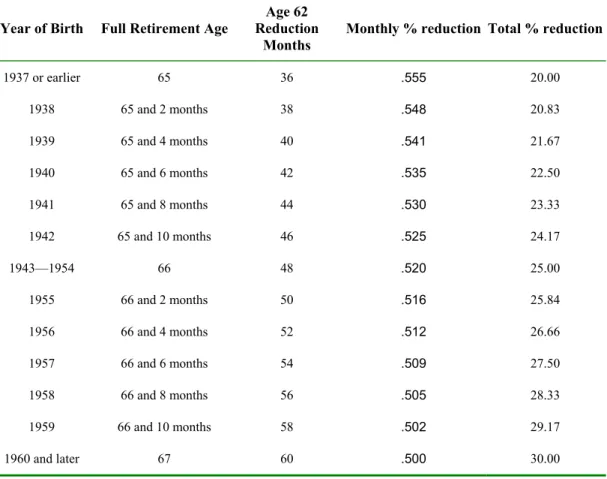
Finally in the USA individuals qualify for an OASI pension by working for 40 quarters in covered employment. The early-eligibility age in OASDI is 62, though the "normal retirement age" (youngest age of eligibility for an unreduced or full pension) is 65, (from 2027 this will become 67) for both males and females. Tight actuarial adjustments apply for early retirees (see Table 3). Also, delayed retirement credit (DRC) applies to late retirees, for example for workers reaching age 65 in 2000, an
12 Both in Italy and Spain special allowance are made for some workers if they started working very early or if they were
employed in occupations where health hazards or hard working conditions applied. Also: during periods of recession in some sectors early retirement was a convenient way to make workers redundant at the expenses of the entire economy and special rules would apply to workers in these sectors.
additional 6% is paid for each year of delay; this amount will steadily increase until it reaches 8% per year in 2008.
Table 3: USA. Social Security Full Retirement and Reductions by Age
Year of Birth Full Retirement Age
Age 62 Reduction
Months Monthly % reduction Total % reduction
1937 or earlier 65 36 .555 20.00 1938 65 and 2 months 38 .548 20.83 1939 65 and 4 months 40 .541 21.67 1940 65 and 6 months 42 .535 22.50 1941 65 and 8 months 44 .530 23.33 1942 65 and 10 months 46 .525 24.17 1943—1954 66 48 .520 25.00 1955 66 and 2 months 50 .516 25.84 1956 66 and 4 months 52 .512 26.66 1957 66 and 6 months 54 .509 27.50 1958 66 and 8 months 56 .505 28.33 1959 66 and 10 months 58 .502 29.17 1960 and later 67 60 .500 30.00
Source: USA Social Security Administration
Clearly eligibility rules can explain most of the pattern in terms of the most prominent spikes, however not all of the action in the data comes from these rules and, most importantly, it is not clear how and why workers decide to retire earlier than the normal retirement age. It is useful to contrast the age-profile of the hazard rate with a measure of the incentives provided by the system. In the context of an international project Gruber and Wise (1999) have proposed to consider a summary statistic called the implicit tax on work14. This measures the advantage (disadvantage) to a worker of working an extra year
in terms of additional social security rights built up in that year, relative to the potential earnings of that extra year of work. The numerator of the implicit tax captures a dynamic measure given by the change in the stock of social security wealth (this latter is simply the present value of future benefits, discounting for mortality probabilities) due to the extra year of work, the denominator accounts for the potential extra
14 Gruber and Wise (1999) look at a selected number of countries and guide the methodology through a very tight template based
on micro data, in order to make results comparable. In a similar fashion Blöndal and Scarpetta (1999) contrast early exists form the labor market and implicit tax on work for a large number of OECD countries, hence allowing for more cross-country variation in the data. Both projects reach similar conclusions on the nature and size of the implicit tax and on its importance in explaining early retirement.
earnings accruing to the individual, but also the additional contribution (payroll tax) due. Hence the implicit tax is a summary dynamic index of the main features of the social security system in terms of benefit provision, eligibility and contributions. In Table 4 implicit tax rates have been computed, for a representative worker (man), on a comparable basis over the relevant age range (typically age 55 to age 70, when individuals are “at risk”). Eyeball econometrics suggests, for each country, a non-trivial correlation with the respective hazards: at the ages when the implicit tax is positive (a tax) and jumps to a high level there is an incentive to retire and almost invariably a spike in the hazard occurs, if eligibility rules allow to do so. When the implicit tax is negative (subsidy) there is an incentive to supply labor for an additional year, at that age (hardly ever observed)15.
3.2.2 Benefit computation and other features
From the above discussion it is clear that eligibility rules must be combined with the benefit computation rules in order to fully understand the incentive structure. Some key features paly a role: the actuarial adjustments by age applying to the earnings-related benefits, the existence of flat benefits provisions (e.g. minimum benefits granted in Italy and Spain) and indexation rules.
In Italy, for the period relevant for the micro-data evidence (i.e. before 1993), pensionable earnings for private sector employees were computed on a “final salary” basis a worker could get at most 80% of his pensionable earnings 16. The system was highly progressive because of the existence of both
capping on earnings and a minimum benefit level. The 1992-reform and to a larger extent the 1995 reform substantially changed these rules. In particular the 1995 reform introduced a “notionally defined contribution system”. Crucial elements of the reform are: (i) how the accrued value of the “virtual” fund is computed, (ii) how it is then converted into an annuity at the time of retirement, and (iii) the indexation rule adopted for the pensions outstanding. Besides changing the benefit formula and the eligibility rules, the 1995 reform also took a number of steps in the direction of unifying the rules of the many schemes in which the Italian social security system is organized. It should be mentioned that between 1992 and 1997 there have been spells (typically lasting between 6 months and 1 year) in which many employees were not allowed to take early retirement17. Note that people will retire under the pre-1993 system until about the
year 2015. During the following 15-20 more years, an increasing fraction of a retiree's pension will be computed on the basis of the 1992-system. It will only be around 2030 that a significant number of workers will start retiring fully under the 1995 rules.
In Spain, if eligibility conditions are met, the initial pension of a worker retiring at age 65 is proportional to the benefit base (base reguladora), a weighted average of covered earnings during the last 8 years before retirement . Outstanding pensions are fully indexed to price inflation, as measured by the consumer price index. Pensions are subject to both a ceiling and a floor, both legislated annually. The 1997-reform harmonized the different funds, increased the number of years entering the benefit base. Moreover, the factor converting the benefit base into the pension amount is now equal to 60 percent plus 3 percent for each year of contribution between 15 and 25, to 80 percent plus 2 percent for each year of contribution between 25 and 35, and to 100 percent after 35 years of contribution. Finally, workers who retire after the age of 60 with 40 or more contribution-years face a penalty of only 7 percent (rather than 8%) for each year under age 6518. In the USA earnings-related benefits are granted if 15 years of
contributions have been completed. Benefits are determined in three steps. The first step is computation of the worker's Averaged Indexed Monthly Earnings (AIME), which is 1/12th of the average of the worker's annual earnings in covered employment, indexed by a national wage index. Importantly, additional higher earnings years can replace earlier lower earnings years, since only the highest 35 years
15 Note that small negative values are obtained for the US at ages 62 and 63: the interpretation is that after having passed the age
of early eligibility (age 62) it is convenient to wait until age 65.
16 Details of the systems and of their reforms can be found in Brugiavini and Peracchi (2001) and Franco (2002).
17 The 1995 reform has gradually removed these constraints. In the transitional phase starting in 1996 public sector employees
who claimed early retirement benefits suffered minor reductions on the basis of actuarial adjustment factors.
of earnings are used in the calculation. The second step is to convert the AIME into the Primary Insurance Amount (PIA). This is done by applying a three-piece linear progressive schedule to an individual's average earnings. As a result, the rate at which SS replaces past earnings (the "replacement rate") falls with the level of lifetime earnings. The third step is to adjust the PIA based on the age at which benefits are first claimed. For workers commencing benefit receipt at the Normal Retirement Age (legislated to rise slowly from age 65 to 67 over the next twenty years), the monthly benefit is the PIA. For workers claiming before the NRA, benefits are decreased as explained above (or increased for delaying retirement). Hence for example claiming at age 62 provides a benefit which is 80% of the full retirement benefit. While a worker may claim as early as age 62, receipt of SS benefits is conditioned on the "earnings test" until the worker reaches age 6519.
We do not discuss here a number of important differences in the social security system of the three countries, for example the role of family considerations (the US system features a “dependent wife” additional benefit), the intricacy of the application of minimum benefits and capping, the differential treatment of different public funds (in Italy private sector versus public sector funds) and the differential treatment offered to different generations (in Italy the application of the transitional rules). However an important feature of the social security system (or of the welfare system) should be mentioned, i.e. the existence of alternative exit routes.
Brugiavini and Peracchi (2001) argue that for Italian workers the transition is currently from work to retirement. Many other “soft landing” or bridging plans exist, but they would all fall in the category of “pre-retirement” or “early-retirement” and, in the Italian micro data, they would effectively correspond to retirement. As far as disability benefits are concerned, after the changes legislated in 1984, their importance as an escape route has greatly diminished20. In Spain unemployment benefits (UB) are granted, conditional on a previous spell of contributions, and are available only for workers in the RGSS. There are two continuation programs for those who have exhausted their entitlement to contributory unemployment benefits: one for those aged 45+ and the other for those aged 52+. The latter program is a special subsidy for unemployed people that are older than 52, lack income sources, have contributed to unemployment insurance for at least 6 years in their life and, except for age, satisfy all requirements for an old-age pension. The Spanish system also provides insurance against both temporary and permanent illness or disability. Benefits are more generous than for the old-age program because they are not subject to penalties for early claim or insufficient years of contribution, and only depend on approval by a medical examiner (notoriously, the criteria used by examiners varies both over time and across regions). Since the early 1990s, access to disability benefits has been tightened and, contrary to the practice prevailing during the 1980s, it is now uncommon to access permanent benefits after age 55. This has mainly been achieved by lengthening the disability evaluation process for temporary illness, which in the past was most often used as a bridge to retirement21. Finally, in the USA a retiree who qualifies for disability insurance benefits receives full pension benefits with no reduction even at early ages.
These examples suggest that comparing retirement (and early retirement) across countries misses the important point that there may be “pathways” to retirement characterized by different benefit provisions. For example a worker could claim disability benefits (if eligible) and subsequently move into old age benefits. In some cases, the combination of different welfare policies creates loopholes for workers to permanently leave the labor force, though these workers are not officially retired. In this sense a better grasp of the actual fraction of workers who retire could be gained by measuring inactivity rates (see Table 8) or labor force participation. Whatever measure one is using, it is clear that workers leave the labor force well before the normal retirement age: older workers in Italy and Spain leave the labor force at younger ages than they do in the US. As Gruber and Wise (1999) and Blöndal and Scarpetta (1998) point out, this trend is not confined to a few countries.
19 See Coile and Gruber (2001) for details.
20 The fall in disability benefits out of total benefits occurring after 1984 is documented in Brugiavini (1999). 21 For a full description of the availability of these programmes see Boldrin, Jimenez and Peracchi (2001a).
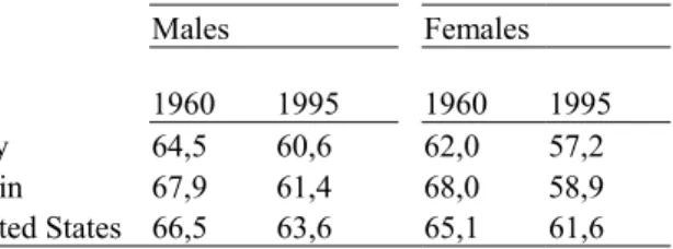
Table 5: Estimates of the average age of transition to inactivity among older workers
Males Females
1960 1995 1960 1995 Italy 64,5 60,6 62,0 57,2 Spain 67,9 61,4 68,0 58,9 United States 66,5 63,6 65,1 61,6
Source: Blöndal and Scarpetta, 1998.
4. Micromodeling of retirement behavior
A simple but useful representation of retirement incentives is provided by the option value model introduced by Stock and Wise (1990). The key feature of the model is the fact that, when deciding on whether or not to retire, a worker compares the expected value of retiring immediately with the expected value of continuing working. More precisely, based on the available information, a worker computes the expected value of retiring at any future date. The difference between the maximum of these expected values and the expected value of retiring today is called the option value of postponing retirement. If the option value is positive, the optimal decision is to continue working. Otherwise, the optimal decision is to retire. In two related projects Gruber and Wise (1999 and 2001) have suggested a common framework to implement a tractable version of the option value model across different countries. While in the first project (1999) the attention is focused on a representative individual (a male worker characterized by the median earnings of his cohort) for each country, in the second project (2001) the authors intend to exploit variability both between countries and within countries. Results from Gruber and Wise (1999), coupled with the research carried out at the OECD by Blöndal and Scarpetta (1998), has prompted the attention of economists and policy makers on the relevance of early retirement, an issue mostly neglected in the policy debate. The approach taken by Gruber and Wise (2001) in their more recent project is focused on the role of the incentives at the individual level and it requires micro data for workers observed at different ages. It should be mentioned that we make use in this paper of results obtained in this latter project, which is still work-in-progress. In particular, preliminary results are drawn from the work of Brugiavini and Peracchi (2001) for Italy, Boldrin, Jimenez and Peracchi (2001b) for Spain, and Coile and Gruber (2001) for the USA. Hence the evidence should be interpreted with care.
4.1 The Option Value model: a reduced form approach
In this section we briefly describe the Option Value model for retirement decisions and we propose a simplified version as suggested by Gruber and Wise (2001). For a formal description of the Option Value model, consider a worker of age a, where a is greater or equal to the early retirement age. A worker who decides to work until age r > a, expects to earn Ws in each year s until retirement and then to receive a pension equal to Br(s) until the age of death S. The pension benefit depends on the retirement
age r, past work history and the pension rules. We assume that, when deciding on whether or not to retire at age r, the worker evaluates the indirect utility of the stream of future income as follows
(1)
∑
∑
= − − = −+
=
S r s s a s r a s s a s ar
U
W
U
B
r
V
(
)
(
)
2(
(
))
1 1β
β
where β is the discount factor, U1(W) is the indirect utility of future earnings and U2(B) is the indirect
utility of future pension benefits. Evaluated at age a, the gain of postponing retirement until age r > a is given by
(2)
G
a(
r
)
=
E
a[
V
a(
r
)
]
−
E
a[
V
a(
a
)
]
where Ea denotes the expectation operator based on the information available up to age a. Let Ya be a
binary indicator that takes value 1 if a worker decides to retire immediately and value 0 otherwise, and let
r* = argmaxr Ga(r) be the age at which the gain of postponing retirement is highest. Because the event
that Ya = 1 is equivalent to the event that:
(3)
G
a(
r
*)
=
E
a[
V
a(
r
*)
]
−
E
a[
V
a(
a
)
]
≤
0
the probability that a worker retires at age a is
(4)
P
(
a
)
=
Pr
{
Y
=
1
}
=
Pr
{
G
(
r
*)
≤
0
}
a a
The model is completed by specifying the indirect utility functions as:
(5)
U
1(
W
s)
=
W
sγ+
ω
s andU
2(
B
s)
=
[
k
(
B
s(
r
)
]
γ+
ξ
swhere the error terms are zero-mean random individual effects. The parameter k captures the fact that the indirect utility of income may be different for a worker and a pensioner. The model may be estimated by the method of maximum likelihood after specifying stochastic processes for the error terms.
A simplified version of the model is particularly convenient from the viewpoint of estimation. Substituting the chosen specification of the preferences in the definition of Va(r) and assuming that the
error terms are equal to zero, by specifying values for the parameters, the value of retiring is easily computed. For example, if β = 0.97 (corresponding to a real discount rate of 3%), γ= 1 and k = 1.5, one has (6)
∑
∑
= − − = −+
=
S r s s a s r a s s a s ar
W
kB
r
V
ˆ
(
)
β
γβ
[
(
)]
γ 1)
)
(
(
97
.
0
5
.
1
)
(
97
.
0
1∑
∑
= − − = −+
=
S r s s a s r a s s a sW
B
r
and one obtains the estimated option value of postponing retirement. This value in turn may be inserted as an additional covariate in a logit or probit model for the probability of retirement. The main advantage of an OV model is its tractability. As shown by Lumsdaine, Stock and Wise (1992), sub-optimal but relatively simple decision rules, such as the ones adopted in OV models, may provide better approximations to the actual choice behavior than the ones implied by model that are fully optimal but harder to compute, such as dynamic programming models.In order measure the option value of postponing retirement it is necessary to define social security wealth:
(7)
∑
+ ==
S h s s s hB
h
SSW
1)
(
ρ
,where S is the age of certain death, s
a s s
β
π
ρ
= −is a discount factor that depends on the rate of time discount ß and the survival probability
π
s at age s conditional on being alive at age h, and B(h) isthe pension benefit expected at age s≥ h+1 in case of retirement at age h. Pension benefits are net of income taxes.
Given this definition of SSW, accrual is defined as
(8)
[
(
1
)
(
)
]
1 1(
)
2 1SSW
B
a
B
a
B
a
SSW
SSA
S a a a s s s s a a a + + + = +−
=
+
−
−
=
∑
ρ
ρ
.The rescaled negative accrual
τ
a =−SSAa/Wa+1, where Wa+1 are expected net earnings at age a+1based on the information available up to age a, is called the implicit tax/subsidy of postponing retirement from age a to age a+1.
While the peak value is:
(9) PVa = maxh
(
SSWh −SSWa)
, h = a+1,..,R ,where R is the mandatory retirement age.
The structure of the application presented in this paper is carried out for each country exactly in the same fashion and the assumptions regarding parameter values are also the same (a real discount rate of 3%, γ= 1 and k = 1.5)22. On suitable micro data estimates of future social security entitlements can be
obtained by carefully taking account of the current (and past) legislation. On the basis of these estimates it is possible to then work out the probability of retirement at a given age implied by the option value model by making use of “dynamic variables” capturing social security incentives in each country. This probability can be estimated over all potential retirement ages (e.g. for Italy the population at risk is in the age range 50-70). The application requires therefore a number of steps: first an estimate of age-earnings profiles for each worker in the sample over all potential ages, then the imputation of future benefits on the basis of the relevant legislation and finally the implementation of the econometric estimates of retirement probabilities. It is particularly important to stress the relevance of this exercise in looking at possible hypothetical or actual reforms: not only the researcher can simulate the first order effects of social security reforms due to changes in benefit accrual and eligibility rules (an exercise which the social security administration of each country is likely to implement already) but she can also assess behavioral effects, which imply changes in retirement patterns due to the reform. In other words the researcher can fully capture the labor market effects.
22 Note that some of these parameters (particularly the parameters of specification 6 ) could be estimated jointly within the OV
model. However, in order to draw cross country comparisons, it proved crucial to impose the same values for all countries. Obviously these values may be unsuitable for some countries and some sensitivity analysis would be required. Some sensitivity analysis has been carried out for some alternative specifications and results are available upon request from the authors.
4.2 Data selection, definition of retirement and earnings projections
A first issue is the definition of retirement and the identification of this state in the data. In any given year t, being retired can be characterized by a number of different events. Correspondingly, we have different definitions of retirement, which can be implemented on panel data. E.g. not having a working spell after year t (exit from the sample into an absorbing state). In addition to this, one may check that the individual is not receiving wages (paying contributions) in years t+ kk, >0. In addition, one could have information on the termination of the spell corresponding to an actual transition on to retirement.
For Italy, Brugiavini and Peracchi (2001) implement the econometric procedure by making use of a random sample of workers observed each year between 1973 and 1994, who are employees in the private sector drawn from the social security administrative records – INPS-FPLD Archive (see data Appendix). Unfortunately, one is unable to distinguish between exits from the archive due to actual retirement, to death or to other factors (e.g. moving to self-employment). For the cohort at risk retirement and death are the two major exit routes. Also for Spain use is made of social security files, HLSS (see the Data Appendix and Boldrin, Jimenez and Peracchi, 2001b) also in the form of a long panel. In the Spanish application, the analysis is carried out for workers born between 1916 and 1958. While there is practically no restrictions on the labor market participation sample, which covers all the Spanish social security regimes, the wage sample is restricted to individuals enrolled in the major funds. For the USA, Coile and Gruber (2001) select a sample from the Health and Retirement Survey (HRS) panel for individuals aged 55 to 69.23
The specification of a model for the age-earnings profile represents an essential step in the estimation of social security wealth at the individual level. Note that this requires stretching considerably out of the sample to cover the entire working history from the first year of contribution (say 20) to the last potential retirement age (say 70): no sample could possibly contain all these data points. Results could be very sensitive to the way earnings projections, in particular backward projections, are carried out. For example, what may seem a negligible overestimation of real earnings in the early years can have marked effects on benefit calculations when the whole earnings history matters for benefit computation (like in the USA). A common (to all three countries) problem is to account for part-time work or partial retirement typically occurring after age 55, which would produce a downward bias in the estimates of the age-earnings profile. For this reason a simple approach is to assume that after a given age (say age 55) real earnings grow at a constant rate. Hence, the general strategy to model earnings profiles is as follows: each country has estimated a model for earnings growth at individual level, which would best fit the data in order to fill any gap within the sample period (and before age 55, say); when going backward, out-of-the-sample fitted values are obtained either through the estimated individual earnings equation or through wage growth rates drawn from national accounts data; finally forward projections assume a flat real age-earnings profile starting at age 55.
In particular, for Italy, Brugiavini and Peracchi (2001) assume that individual real age-earnings profiles are completely flat after age 55. Before age 55, if earnings are not observed, an imputation is made on the basis of fitted earnings24. When going backward, using a flat earnings profile would grossly
overestimate the level of earnings at earlier ages and grossly underestimate real earnings growth. To avoid this problem, individual earnings are assumed to grow at the annual growth rate of aggregate earnings. For Spain, Boldrin, Jimenz and Peracchi (2001b) face an additional problem as they do not observe earnings directly, but only covered earnings. Covered earnings are a doubly censored version of earnings for employees, while they are very weakly related to true earnings for workers in self-employment.
23 For the precise definition of a transition from work to retirement see Coile and Gruber (2001).
24 In Brugiavini-Peracchi (2001) simple non parametric interpolations have been preferred to fixed-effects-AR models for
Proper account is taken in their paper of the top-censoring problem present in the data, which may seriously alter the results of the econometric exercise.
4.3 Estimating social security wealth and incentive measures
For a worker of age a, social security wealth (SSW) is defined in case of retirement at age h ≥ a as the expected present value of future pension benefits. Given the SSW, the three incentive measures for a worker of age a are.
1. Social security accrual (SSA) is the difference in SSW from postponing retirement from age a to age
a+1.The SSA is negative if the expected present value of pension benefits foregone by postponing
retirement by one year is greater than the expected present value of the increment in the flow of pension benefits.
2. Peak value: the peak value is the maximum difference in Social Security Wealth between retiring at future ages and retiring at the current age.
3. Option value: is the maximum utility difference between retiring at future ages and retiring at age a. These three incentive measures are consistent with the view that, in deciding whether or not to retire, a worker compares the expected gain from each of the two alternatives. Note that, in computing the incentive measures, the correct (but laborious) assumption is that workers revise their expectations at each age. Hence for each given age, a worker projects the path of observed earnings according to the model and then computes her SSW and the incentive variables taking into account the information currently available. This requires re-computing SSW and the corresponding incentive measures for each year until retirement. Reforms are assumed to come as a surprise to workers. The estimates of social security wealth (excluding occupational pensions) is carried out consistently in the three countries, however in each country the rules provided by the system had to be implemented.
For Italy, in the actual calculation of SSW Brugiavini and Peracchi (2001) look at ages 50 to 70 and assume a real discount factor of 3 percent. Benefits are defined in real terms and the indexation rules prevailing under each legislation are implemented (e.g. before the 1992 reform indexation to both price inflation and real wages). Given administrative records with no information on marital status, estimates of SSW for men and women are obtained separately under the assumption that these are single workers. For Spain, the assumption is made that starting at age 55 and until a person reaches age 65, there are three pathways to retirement: the Unemployment benefit program, DI benefits and early retirement. At each age, an individual has an age-specific probability of entering retirement using any of these three programs. In the USA, the SS incentive variables incorporate dependent spouse and survivor benefits, since these are important components of SSW. For a worker with a non-working spouse, these benefits are based solely on the worker’s earnings record. For a worker whose spouse is entitled to benefits on his/her own, the spouse’s benefits are based (partially or fully) on the spouse’s record but are also included in SSW. For the simulations, it is assumed that workers claim SS benefits at retirement, or when they become eligible (age 62) if they retire before then. Private pension incentives are not incorporated into the analysis, although, as we already argued, results may differ significantly from those for social security alone, because the primary goal is to discuss the impacts of public pensions on retirement.
4.4 Predicting retirement and simulating the effect of “hypothetical reforms”: modeling choices and results
We have seen that the hazard rates exhibit for all three countries some important spikes. The challenge in predicting exits at each given age, given the option to post-pone retirement, is to capture the pattern observed in the data. Therefore, turning to the estimation of the probability of retirement, this is related to the incentive variables, age dummies and other covariates. To be more precise, the incentive variables are included in a probit regression (along with other important covariates) to estimate retirement probabilities. The strength of the Gruber-and –Wise-approach is that the estimation procedure and the specification of the model are exactly the same in all countries. The intuition for this modelling strategy is that the incentive variables and the level of social security used as explanatory variables capture the effects of the social security system (including dynamic incentives), conditioning on other characteristic of the worker, while the age dummies capture any residual age effect coming from preferences and/or social norms.
For all three countries estimates of social security wealth and incentive variables are obtained under three alternative regimes. These intend to provide, along the status quo, two illustrative reforms in order to assess the potential behavioral response embedded in each social security system with the respect to a current benchmark. The motivation for designing these hypothetical reforms is to look at the effect on retirement decisions of a reform which shifts the legislated retirement age by three years (first hypothetical reform), hence imposing on the data a delay in the retirement age. This is compared to a reform that, by adjusting benefits on actuarial basis, acts more directly on the dynamic incentives (second hypothetical reform). These reforms may never materialize in practice and they may not produce the same results across countries: the idea is to implement exactly the same changes, though the status quo may obviously vary across countries.
In particular, the first policy simulation focuses the attention on a simple change in the eligibility rules (postponing retirement ages) and the second stresses the importance of age-neutrality (or non neutrality) of the system by applying age-specific actuarial penalties (subsidies) to early (late) retirement. Hence the regimes are:
1 The baseline regime, in all the three countries this is the regime prevailing in the current years.
2 R1. Policy simulation-1. Starting from the current system (the baseline case), raise the normal retirement age by three years while holding constant all other features.
3 R2. Policy simulation-2. This simulation entails a different pension program altogether, which features an early retirement (say age 60) and a normal retirement age (say age 65). It provides a retiree with a benefit, which replaces 60% of her projected earnings when she turns 65. It applies an actuarial reduction of 6% per year for early claiming and an actuarial increase of 6% per year for later claiming. It essentially makes early retirement costly and introduces age-neutrality in retirement choices.
First it should be noted that the first simulation (R1) is a change relative to the status quo, hence it entails a change for all countries. The second simulation (R2), instead, imposes a new design of the pension system, independently of the current baseline. This implies that some countries may be very far from the second policy regime in their actual system (baseline) while others may already implement a system similar to that envisaged by R2. For example, while the Italian system features an actuarially unfair regime for the baseline scenario, both for Spain and the USA we could argue that actuarial fairness basically holds in the baseline. Indeed the USA system is less generous than the policy simulation-2 (see Coile and Gruber 2001), so that for the USA, simulation 2 should increase the incentives to retire early.
The first step of the application is to predict exit probabilities for the baseline (status quo scenario). To this end a probit regression is carried out (for each country) under the baseline scenario for the three incentive measures (accrual rate, peak value and option value). Note that all countries different specifications are attempted of the retirement model: all specifications include the incentive variable (i.e.
the accrual, the peak value or the option value are used as alternatives) and some basic demographics, but age may enter the equation in different fashions. The simplest specification is based on a linear term for the age variable (denoted as specification M1). A second specification includes a full battery of age dummies (specification M2), while a third specification (M3) makes use of a polynomial in age with age dummies on the relevant spikes. A discussion on the advantages and disadvantages of these models can be found in Brugiavini and Peracchi (2001), in this paper we limit ourselves to a description of the results for a selection of cases.
The second step is to introduce the hypothetical reforms: the effects of the alternative regimes is modelled by simulating, i.e. by changing the level of the social security wealth, of the incentive measures and of the eligibility rules according to the hypothetical reforms, other things being equal. Obviously comparisons between the baseline (current pension system) and the hypothetical reform are carried out by making use of the same model, for example by making use of the full set of age dummies (M2) for all policy regimes. In order to fully capture the effects of these hypothetical reforms not only the age dummies are used but they are also adapted to reflect the impact of the policy change. For example, in the case of the hypothetical reform corresponding to a 3-years shift from the baseline the social security wealth variable and the incentive variables change according to the policy change under consideration and the age dummies are shifted accordingly. This “modified” model M2 is referred to as model S3 in the application. Hence, for Italy, the effect of the age dummy at age 60 should apply at age 63 under the hypothetical reform, so that the spike in the hazard effectively shifts by three years. It should be added that the econometric specification captures dynamic incentives both by looking at possible wealth effects (changes in social security wealth) and by looking directly at changes in the lifetime profile of the incentives (changes in the accrual, peak value or option value). The combination of these effects may produce several patterns of responses in the retirement decision at the individual level.
In this paper we do not report results of the econometric models. Furthermore, we limit ourselves to discuss qualitatively the results of the simulations carried out for Spain and the USA, while presenting some more details for Italy as an example of the application.
Results for Spain and USA
For Spain, in almost all cases, the impact of the hypothetical reforms varies across both simulation exercises and choice of the incentive measures (accrual, peak and option value) as well as gender, effects are typically more marked for men than for women. 25 First, the R1 hypothetical reform
has little impact on retirement behavior; when it does, it implies an increase of the average retirement age between 0.69 years (option value specification) and 1.58 years (accrual specification). The R2 reform has a very limited impact on retirement ages in all cases. Hence, by and large, the Spanish pension system seems to feature rules which are already “actuarially fair” as no substantial change in retirement ages is achieved by moving to a system which has in place an actuarially adjustment of benefits, while a slightly more significant change is achieved by imposing a delay in retirement.
For the USA, the peak value and option value both have a significant negative effect on the retirement decision. The first policy change, (shifting retirement age -R1), would have the effect of lowering the average retirement rate for both men and women. The second policy change (actuarial adjustment-R2), has a somewhat different pattern of effects. First of all, it significantly raises, rather than lowering, retirement rates, also, unlike the effects of the first reform, which fade over time, these impacts are constant or grow at all ages, reflecting the fact that this policy does not so much shift incentives towards earlier retirement as it does raise the wealth level of retirees at all ages.
Results for Italy