A TWO-STEPS METHOD TO BALANCE
A SQUARE MATRIX
MARCO RAO Development of Particle Accelerators and Medical Applications
Physical Technologies for Safety and Health Division Fusion and Technologies for Nuclear Safety Department
FrascatiResearch Centre,Rome
RT/2016/17/ENEA
ITALIAN NATIONAL AGENCY FOR NEW TECHNOLOGIES, ENERGY AND SUSTAINABLE ECONOMIC DEVELOPMENT
MARCO RAO
Development of Particle Accelerators and Medical Applications Physical Technologies for Safety and Health Division Fusion and Technologies for Nuclear Safety Department Frascati Research Centre, Rome
A TWO-STEPS METHOD TO BALANCE
A SQUARE MATRIX
RT/2016/17/ENEA
ITALIAN NATIONAL AGENCY FOR NEW TECHNOLOGIES, ENERGY AND SUSTAINABLE ECONOMIC DEVELOPMENT
I rapporti tecnici sono scaricabili in formato pdf dal sito web ENEA alla pagina http://www.enea.it/it/produzione-scientifica/rapporti-tecnici
I contenuti tecnico-scientifici dei rapporti tecnici dell’ENEA rispecchiano l’opinione degli autori e non necessariamente quella dell’Agenzia
The technical and scientific contents of these reports express the opinion of the authors but not necessarily the opinion of ENEA.
A TWO-STEPS METHOD TO BALANCE A SQUARE MATRIX M. Rao
Riassunto
Questo lavoro presenta un metodo semplice e intuitivo per bilanciare una matrice quadrata, basato su una normalizzazione della matrice, e sulla distribuzione lungo le diagonali della stessa di due quantità: la media aritmetica degli incrementi nei totali marginali e la differenza tra i nuovi totali ottenuti e i totali desiderati. Il metodo è stato testato su una sequenza di matrici quadrate bilanciate generate casualmente, applicando alle stesse delle variazioni nei totali marginali casualmente distribuite secondo una uniforme continua.
Parole chiave: Matrici quadrate, Bilanciamento, metodo a due passi.
Abstract
This work deals with a simple method to balance a square matrix, based on a normalization of the matrix, and on the distribution on its diagonals of two quantities: the arithmetic mean of the margi-nal total change and the difference between the resulting totals and the fimargi-nal objective. The method was tested on a sample of balanced matrices randomly generated using an uniform continuous distribution.
1. Introduction 2. The method
2.2 Comparison with RAS method 2.2.1 Brief note on RAS 3. Conclusions Bibliography 7 7 10 10 14 16 INDEX
Pag 7 1 Introduction
The balancing of a square matrix is a well-known problem in economics (Miller & Blair, 2009), mathematics and statistics (Deming & Stephan, 1940), (Bacharach, 1965), (Fienberg, 1970), (Pukelsheim & Simeone, 2009).
This work presents a simple method based on two subsequent steps to balance a square matrix of any dimension due to changes in its marginal totals (m.t.) namely the total of its rows and columns, under the condition:
The method was call 2-sBM (2-step Balancing Method).
2 The method
Observing a matrix composed by elements all equal to 1, we can see that every changes of 1 unit in the marginal totals can be handled using the main or the secondary diagonal. Let's see the example for a 3 x 3 matrix:
1 1 1 3 1 1 1 3 1 1 1 3 3 3 3 1 1 2 4 1 2 1 4 2 1 1 4 4 4 4 1 1 3 5 1 3 1 5 3 1 1 5 5 5 5 … and so on.
Pag 8 To be more precise, each diagonal of the matrix can handle every increase of 1 unit in each m.t. by increasing of 1 its elements: this suggest that any increase in m.t. could be handled in easier way respect to other mechanical procedures like RAS (see section 2.2) that is based on modification of values for the entire matrix.
To demonstrate what above mentioned, we start from a simple 3x3 matrix, randomly generated1. Numbers are reported with 10 decimals in order to show the accuracy in results. Before the application of method, we have to prepare the matrix, to escape from the particular case of matrix composed by all 1.
Let’s start to a simple matrix like the Start Matrix below. The first operation is to normalize such a matrix using one of the m.t. (the total of the 3rd row for example, reported in bold) as Reference Value, in order to calculate a Normalized Matrix (NM).
So, we begin from a Start Matrix (SM) randomly generated (difference between the m.t. of rows and columns are reported in italic red)
67,0000000000 99,0000000000 78,0000000000 244,0000000000 139,0000000000 39,0000000000 28,0000000000 206,0000000000 38,0000000000 68,0000000000 77,0000000000 183,0000000000 244,0000000000 206,0000000000 183,0000000000 0,0000000000
then, we divide every value in the matrix for the Reference Value to obtain the NM required:
0,3661202186 0,5409836066 0,4262295082 1,3333333333 0,7595628415 0,2131147541 0,1530054645 1,1256830601 0,2076502732 0,3715846995 0,4207650273 1,0000000000 1,3333333333 1,1256830601 1,0000000000 0,0000000000
1 For each cell of the matrix generated is: a
ij= Int((100 - 1 + 1) * Rnd + 1) where aij is the element of row i and column j. The formula is coming from an arbitrary choice made only to simplify the demonstration of the method.
Pag 9 Now, let’s suppose to change the marginal totals introducing a random fluctuation between 0 and 1 in them (we have to sum this fluctuation on old totals), to obtain the results reported in phase 3 in blue (the fourth number is the sum of fluctuation, on the basis of which we calculate the arithmetic mean of the random changes, AMRC).
0,3661202186 0,5409836066 0,4262295082 1,3333333333 0,0090452142 0,7595628415 0,2131147541 0,1530054645 1,1256830601 0,6808660730 0,2076502732 0,3715846995 0,4207650273 1,0000000000 0,0330982483 1,3333333333 1,1256830601 1,0000000000 0,0000000000 0,7230095354
Now the matrix is ready for the application of the method. The 1st step involve the sum of AMRC and each value on the secondary diagonal of the matrix (values in red).
2) +AMRC
where is the element of the secondary diagonal relative to row i and column j.
Doing so, a Differential between the Marginal Totals (DMT) of the new balanced matrix and the final one is immediately created (in green).
0,3661202186 0,5409836066 0,6672326867 1,5743365118 1,3423785475 -0,2319579643
0,7595628415 0,4541179326 0,1530054645 1,3666862386 1,8065491331 0,4398628945
0,4486534517 0,3715846995 0,4207650273 1,2410031785 1,0330982483 -0,2079049302
1,5743365118 1,3666862386 1,2410031785 0,0000000000
In order to obtain the results that we want, all we have to do is to distribute DMT on the main diagonal of the matrix, using the simple formula:
3)
Pag 10 2nd step 0,1341622543 0,5409836066 0,6672326867 1,3423785475 0,7595628415 0,8939882710 0,1530054645 1,8065491331 0,4486534517 0,3715846995 0,2128600971 1,0330982483 1,3423785475 1,8065491331 1,0330982483 0,0000000000
As we can see, the new matrix is perfectly balanced at desiderated values of the new marginal totals.
Now it’s immediate to calculate a results in the same order of the initial values of SM:
24,5516925315 99,0000000000 122,1035816616 245,6552741930 139,0000000000 184,2003148309 28,0000000000 351,2003148309 82,1035816616 68,0000000000 38,9533977735 189,0569794350 245,6552741930 351,2003148309 189,0569794350 0,0000000000
At practical level, the method is immediate: all we have to do is to prepare a spreadsheet to perform the requested operation of preparation from 1 to 3 and the two requested by the method, then generate a matrix or import a predefined one and set the desiderated changes in m.t.
2. 2 Comparison with RAS method
It can be useful compare 2-sBM with other existing method. In order to balance a square matrix, we recall that the RAS method (Miller & Blair, 2009) is a widely known and commonly used automatic procedure for balancing national accounting matrices (Fofana, Lemelin, & Cockburn, 2005): a quick note on such a procedure is provided in the follows. The subsequent step will be a quick comparison between 2sBM and RAS.
2.2.1 Brief note on RAS
The amount of statistical information required for the construction of an input-output table, or a Social Accounting Matrix (U.N., 1968) is significant, so national statistics institutes
Pag 11 generally perform this kind of work only every 4-5 years (Di Palma, 2005). Through this period, an estimate of changes in the matrices is performed using several methods: the RAS is the most popular and applied (Parikh, 1979).
The general methodology can be summarized in the following phases: firstly, it is necessary to evaluate the "marginal totals" of the table, i.e. the sum of rows and columns of the intermediate flows matrix: this involves the construction, for each branch, of the goods and services equilibrium account, the production account and the value added distribution account. We skip for practical reasons the part relative to the price updating of matrix.
We start from the system modification due to changes in the absorption (r) and fabrication (s) degrees of each good2. To perform this, each technical coefficients modified in the previous step, , will be multiplied for (r) and (s). In matrix notation we can write: where: is the technical coefficients matrix modified from (r) and (s) effects on each good is the diagonal matrix that take account of the variations in the sales (r), is the diagonal matrix of the price index between base year and update year and diagonal matrix that take account of the variations in the fabrication processes (r) The updated coefficients can be writing as follow:
4.
Substituting with we have: 5.
And, then the new value added coefficients:
6.
The elements of (r) and (s) matrix are obtained by an iterative procedure based on a set of economic variables at the base year: X gross production, M imports of goods and services, V value added at factors cost, T indirect taxes, C public and private expenditures, I gross investment, E exports of goods and services. On the base of the above dataset, we determine the totals of purchases and sales of intermediate goods, and the marginal distributions of the table:
2
Pag 12 7.
8.
where: is sales of goods and services of sector i to other sectors purchases of goods and services of sector i from other sectors. Calculation of the above vectors starts from the matrix (A*) multiplied by the production vector with respect to the constraint represented by U, until the iterative process, after a certain number of steps, gives (r) and (s). Formally, at year t:
9.
10.
Where the symbols are already defined and I is the identity vector.
At matrix is obtained by A* as follow:
10.
Generally : to get the second term equal to both terms are divided by and multiplied times ; so:
11.
The product is a further correction of the original matrix : we can satisfy the other condition ( ) operating:
12.
Normally and to get the equality between the two expressions we divide both the terms by then multiply hem times . We get:
13.
Pag 13 14. then: 14. repeating 13: 15.
To match with the z vector we have:
16.
After (k+1) iterations, for sales and purchases vectors, the follow relationships are obtained:
18.
19.
Fixing a suitable threshold, the iteration process will converge to a finite solution.
At the last iteration, the resulting matrix will be as follows:
20.
The r and s vector will be calculated by the following expressions:
21.
22.
The iteration process continues until rows and columns totals reach an acceptable difference threshold. The research on iterative proportional fitting procedures was firstly related to a probabilistic class of problem in the first half of the last century (Deming & Stephan, 1940), then it was extended to other mathematical problems and finally demonstrated (Fienberg, 1970).
Pag 14
3 Conclusions
The Start Matrix at page 8 has been balanced also with traditional RAS method. Since the RAS handle negative values with difficult3 (a minor problem in economics), 2-sBM is preferable: furthermore, the problems of RAS with negative values could be a limit in other kind of applications. However, using only matrices with all positive values (in order to make the comparison) a Monte Carlo simulation of balancing reports the following results:
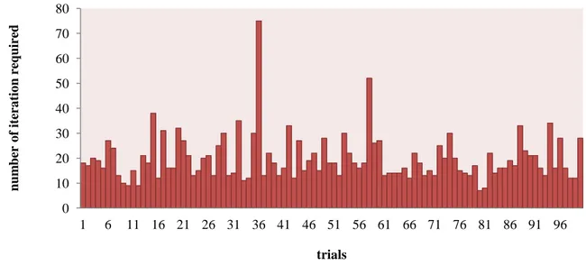
Table 1 - Main statistics about number of iterations required to balance 3x3 matrices randomly generated from a sample of 1000 trials number of iterations mean 20,8 St. dev 10,6 min 7,0 max 163,0
Figure 1 - Number of iterations required to balance randomly generated 3x3 matrices (first 100 matrices)
2-sBM is clearly more efficient, since the arithmetic mean of the number of iterations required using RAS in the simulation is ten times the operations required by it.
3
In order to converge to solution. 0 10 20 30 40 50 60 70 80 1 6 11 16 21 26 31 36 41 46 51 56 61 66 71 76 81 86 91 96 nu m ber o f it er a tio n r equired trials
Pag 15 2-sBM is generally preferable respect to RAS since can handle negative values without problems. In economics, a RAS balancing appears more reasonable, to maintain the proportion in the coefficients: however, the invariance of matrix (only the diagonals are changed), could be probably helpful in case of balancing under constraints (Rao & Tommasino, 2015).
Pag 16
Bibliography
Bacharach, M. (1965). Estimating Nonnegative Matrices from Marginal Data. International Economic Review , 294-310.
Deming, W., & Stephan, F. (1940). On a Least Squares Adjustment of a Sampled Frequency Table When the Expected Marginal Totals are Known. Ann. Math. Stat , 427-444.
Di Palma, M. (2005). Tecniche di aggiornamento di una tavola delle interdipendenze settoriali. Roma: Università degli Studi di Roma "La Sapienza".
Fienberg, S. (1970). An Iterative Procedure for Estimation in Contingency Tables. Ann. Math. Stat , 907-917. Fofana, I., Lemelin, A., & Cockburn, J. (2005). Balancing a Social Accounting Matrix theory and application. Ville de Quebec: CIRPEE.
Mesnard, L. d. (2002). Failure of the normalization of the RAS method : absorption and fabrication effects are still incorrect. The Annals of Regional Science , 139-144 .
Miller, R., & Blair, P. (2009). Appendix C Historical Notes on the Development of Leontief’s Input–Output Analysis. In R. Miller, & P. Blair, Input-Output Analysis - Foundations and Extensions - Second Edition (pp. 724-737). Cambridge: Cambridge University Press.
Parikh, A. (1979). Forecasts of Input-Output Matrices Using the R.A.S. Method. The Review of Economics and
Statistics , 477-481.
Pukelsheim, F., & Simeone, B. (2009). On the Iterative Proportional Fitting Procedure: Structure of
Accumulation Points and L1- Error Analysis. Augsburg: Augsburg Universitat.
Rao, M., & Tommasino, M. (2015). An analysis of the effects of internal constraints application on the accuracy
measures in projecting a social accounting matrix with iterative methods. The case of Italian SAM for years 2005 and 2010. Roma: ENEA.
ENEA
Servizio Promozione e Comunicazione
www.enea.it
Stampa: Laboratorio Tecnografico ENEA - C.R. Frascati luglio 2016