VERIFICA E VALIDAZIONE SULL’ACCOPPIAMENTO DEL CODICE DI
SISTEMA RELAP5 E IL CODICE DI FLUIDODINAMICA COMPUTAZIONALE
FLUENT APPLICATO SU SISTEMI A PISCINA
Ente emittente Università di Pisa (CIRTEN)PAGINA DI GUARDIA
Descrittori
Tipologia del documento: Rapporto Tecnico
Collocazione contrattuale: Accordo di programma ENEA-MSE su sicurezza nucleare e reattori di IV generazione
Argomenti trattati: Generation IV reactors, Tecnologia del piombo, Termoidraulica dei reattori nucleari
Sommario
This report, carried out at the DICI (Dipartimento di Ingegneria Civile e Industriale) of the University of Pisa, illustrates the activities performed in the framework of the AdP2015 and dealing with the application of an in-house developed coupling methodology between a modified version of RELAP5/Mod3.3 and Fluent commercial CFD code, to a pool system, the CIRCE (CIRCulation Experiment) experimental facility. This document initially call up the coupling methodology used, which was developed and improved in the past years. The main applications of the coupling tool to the CIRCE pool system are the main topic of this report. A simplified model with a 2D CFD domain was employed for the simulation of a long transient, representing a PLOHS+LOFA scenario, and the main results are compared with experimental data. A 3D CFD model of the pool was also developed and used to perform shorter transients, both isothermal and non-isothermal tests. Numerical results are compared with the ones from the simulations with the 2D CFD domain and from experiments. The coupled calculations showed interesting results, with some discrepancy with respect to the experiments, due to some simplifications in the modelling. This outcome gives an input for the improvement of the next simulations. In regards to this, the computational domain of the new test section CIRCE-HERO is under development and is presented in the last part of this document.
Note
Riferimento CIRTEN: CERSE-UNIPI RL 1547/2016
Autori:
N. Forgione, M. Angelucci, D. Martelli, D. Rozzia, F. D'Auria, W. Ambrosini
Copia n. In carico a:
2 NOME
FIRMA
1 NOME
FIRMA
0 EMISSIONE 26/09/16 NOME M. Tarantino M. Tarantino
FIRMA
2
Index
Summary ... 3
1.
Introduction ... 4
2.
Coupling procedure ... 5
3.
Coupled calculations with 2D CFD model ... 7
3.1. Computational Domain ... 7
3.2. CIRCE Test I experiment ... 8
3.3. Boundary conditions ... 9
3.4. Main results of “Test I” ... 9
4.
Coupled calculations with 3D CFD model ... 15
4.1. Computational domain ... 15
4.2. Isothermal test ... 15
4.3. Numerical results of “Test 1” calculation ... 17
5.
CIRCE-HERO model for coupled calculations ... 23
5.1. RELAP5 3.3 nodalization of CIRCE-HERO ... 24
5.2. Geometrical domain for CIRCE-HERO coupled calculations ... 24
6.
Conclusions ... 26
3
Summary
This report, carried out at the DICI (Dipartimento di Ingegneria Civile e Industriale) of the University of Pisa, illustrates the activities performed in the framework of the AdP2015 and dealing with the application of an in-house developed coupling methodology between a modified version of RELAP5/Mod3.3 and Fluent commercial CFD code, to a pool system, the CIRCE (CIRCulation Experiment) experimental facility. This document initially call up the coupling methodology used, which was developed and improved in the past years. The main applications of the coupling tool to the CIRCE pool system are the main topic of this report. A simplified model with a 2D CFD domain was employed for the simulation of a long transient, representing a PLOHS+LOFA scenario, and the main results are compared with experimental data. A 3D CFD model of the pool was also developed and used to perform shorter transients, both isothermal and non-isothermal tests. Numerical results are compared with the ones from the simulations with the 2D CFD domain and from experiments. The coupled calculations showed interesting results, with some discrepancy with respect to the experiments, due to some simplifications in the modelling. This outcome gives an input for the improvement of the next simulations. In regards to this, the computational domain of the new test section CIRCE-HERO is under development and is presented in the last part of this document.
4
1. Introduction
This report describes the work performed at University of Pisa in the framework of the AdP2015 on the application of STH code and CFD code coupled calculations to a pool system.
From 2012, at DICI (Dipartimento di Ingegneria Civile e Industriale) of the University of Pisa, an in-house coupling methodology between a modified version of RELAP5/Mod3.3 and Fluent commercial CFD code have been developed. The first developed coupling method used an explicit scheme for the advancement in time. Coupled calculations were performed with application to a simplified representation of the NACIE facility, with good agreement of the obtained results with experimental data [1]. In 2013 the numerical model was improved modifying the correlations used by the RELAP5/Mod.3.3 system code concerning the thermodynamic properties of lead, LBE and sodium, with several new simulations of the NACIE facility [2]. In 2014 the coupling model was improved with an implicit numerical scheme in order to enhance the stability of the coupling procedure. Also, both the explicit and implicit schemes were parallelized in order to perform multi processor CFD calculations inside the coupled model. Again, experimental data from NACIE facility were used to validate the developed numerical model [3]. In 2015, some modifications were implemented in the coupling methodology, in particular for the management of the exchanged data. The new procedure allowed to reduce the time needed for the data exchange between CFD and STH codes with benefit on the duration of the coupled simulations. Further, the coupled calculations were applied to a pool system (CIRCE facility), using a simplified 2D domain for the CFD simulation [4].
This work focused on thermal-hydraulic analysis on a pool system, with application on the CIRCE facility at ENEA Brasimone. Nevertheless, this report does not include a description of the CIRCE facility, since it could be find in several documents, e.g. [4-5].
STH codes are generally inadequate to investigate mixing and thermal stratification phenomena in large pool systems. On the other, the exclusive use of CFD codes requires excessive computational effort. The coupling between two or more scale thus appears to be a promising technique when the small scale phenomena take place in a limited part of the domain. In this report the simulation of a PLOHS + LOF transient, with the use of a 2D CFD model, is presented in Section 3. Further, a 3D CFD model of the CIRCE facility was developed, both isothermal and non-isothermal tests were simulated and the main results are presented in Section 4. Section 5 describes the developed RELAP5/Mod.3.3 model for the entire facility CIRCE+HERO test section and how it will be modified in order to prepare the computational domain for coupled calculations. The development of a new 3D CFD domain, which is necessary for the same purpose, is also presented in Section 5. The main conclusions of this work are summarized in Section 6.
5
2. Coupling procedure
The logic scheme used for the coupling model is represented in Figure 1. It highlights the thermodynamic variables exchanged at the interfaces between the two domains. This scheme differs from the logic used for applications to a loop system (NACIE) [1-3] and is the same used in [4]. The logic that was used for NACIE coupled calculations was unstable when applied to CIRCE calculations. Indeed, a small variation of the pressure given by RELAP5 at the outlet of the pool resulted in very large variation of the LBE mass rate entering the pool, mainly due to its large dimension [4]. Following the procedure in Figure 1, Fluent gives to RELAP5 the pressures both at the inlet and outlet section of the test section (ICE), while at the same time RELAP5 gives the mass flows (velocities) at the inlet and outlet sections of the pool (CFD domain). The temperature at the exit of the heat exchanger is given by RELAP5 to the Fluent pool inlet and vice versa, the temperature at the interface in the bottom (test section inlet) is given to RELAP5 by the pool outlet section of the Fluent domain. Moreover, atmospheric pressure for the cover gas is set as boundary condition to both the domains: at the top of the pool, in the Volume Of Fluid (VOF) region in the Fluent domain, and at the top of the separator of the test section in the RELAP5 domain. Guaranteed that the depth of the two interfaces is the same for both the domains, so that the pressure due to the column of fluid is correctly considered in both sides, this procedure is stable.
Figure 1: Exchanged variables for the RELAP5–Fluent coupled model for calculation on the CIRCE facility.
The numerical method adopted for the coupled simulation is the implicit scheme shown in Figure 2. It is widely described in [3] and [4] and it has not been modified for this work. In an implicit numerical scheme each inner iteration should be repeated until specified convergence criteria is satisfied.
6
Nevertheless, in order to simplify the programming, a fixed number of inner iterations for each time step could be preferred. As in [3] and [4], also in this study three inner iterations were chosen, following a sensitivity analysis. This choice was a good compromise between CPU time and accuracy of results. The Fluent code is the “master code” and advances firstly by one time step and then the RELAP5 code (slave code) advances for the same time step period, using data received from the master code Fluent.
Figure 2: Implicit coupling scheme.
The logic to manage the Fluent code exclusively from Matlab, developed in [4], was used also in this work and is displayed in Figure 3. An add-on of Fluent called CORBA allows the creation of an interface between Matlab and Fluent as a Server. With this module it is possible to manage the Fluent session from Matlab through TUI specific commands. This method brought about great advantage in terms of the global computational time with respect the method used previously, which required the use of a parallelized User Define Function (UDF) to exchange data between Fluent and RELAP5 [1-3].
7
Figure 3: Coupled code management through the Matlab software.
3. Coupled calculations with 2D CFD model
3.1. Computational Domain
In this work, the system code-CFD code coupled model has been applied to the experimental facility CIRCE. A detailed description of the facility can be found in [4-5]. Basically, the CIRCE facility consists of a main cylindrical vessel, with a diameter of about 1.2 m and 8 m high, filled with about 70 tons of molten LBE. The Integral Circulation Experiment (ICE) test section is placed into the main vessel and comprises a Fuel Pin Simulator (FPS), which represents the Heat Source (HS) of the system, a fitting volume, which allows the hydraulic connection between the HS and the riser. A gas injection system is connected to the riser and provide the hydraulic head to enhance the circulation. A separator is placed at the end of the riser and addresses the LBE flow in the heat exchanger (HX), the heat sink of the system. At the exit of the HX the LBE goes back into the main pool. Further, a Decay Heat Removal (DHR) heat exchanger is placed in the pool and it is hydraulically de-coupled from the primary system.
Figure 4 shows the computational domain with a 2D CFD domain. The ICE test section and the HX are modeled with RELAP5, while the main pool and the DHR are modeled with Fluent CFD code. Initially, a simplified 2D CFD geometrical domain was developed aiming at reducing the computational power required. It is a 2D axial-symmetric geometry, assuming the DHR's axis as axis of symmetry. A detailed description of both the RELAP5 and the Fluent domains, so as the grid independence study and other information are reported in Ref. [4]. The coupling procedure and the logic for the exchange of data between the two domains was previously described in Section 2.
8
Figure 4: Sketch of the computational domain for 2D coupled calculations.
3.2. CIRCE Test I experiment
The “Test I” experiment performed in the CIRCE facility reproduces a PLOHS+LOF accidental scenario [6]. In the CIRCE-ICE facility, the transition from forced circulation (at nominal conditions) to natural circulation is obtained reducing the thermal power generated in the HS, stopping the argon injection into the riser, cutting off the main HX, and activating the DHR heat exchanger. Test I started with a steady state condition at full power (nominal value of 730 kW) and forced circulation. The circulation of the LBE was provided by the natural circulation and enhanced by the gas injection system. During the initial stage the argon flow rate was 1.78 Nl/s and the resulting LBE mass flow rate was about 57 kg/s. The heat was removed by a heat exchanger, where the secondary water entered at 20 °C and a mass flow rate of 0.65 kg/s. The transient was triggered after about 7 hours. The FPS power was reduced to 50 kW and then the gas injection was switched off. At this time, the LBE flow was induced only by the natural circulation component and a LBE flow rate of about 7.5 kg/s established in the facility. Meanwhile, the HX was disabled by closing
9
the injection of the secondary water and the DHR-system was activated. The air mass flow rate through the DHR was about 0.223 kg/s and the air inlet temperature was 20 °C.
3.3. Boundary conditions
The aim of the work was to investigate the capability of the coupled calculation to simulate the main thermal-hydraulics phenomena occurring in a pool system, with particular focus on the transition from forced to natural circulation together with the thermal stratification inside the CIRCE pool. For this reason, the boundary conditions for the calculation tried to reproduce as realistic as possible the experimental ones. Nevertheless, in the simulation, the power input was 95% of the nominal value in order to consider the amount of power effectively released to the LBE inside the ICE section. In fact, part of the supplied electrical power is lost radially or released outside the active region due to losses in the cold tails. So, the initial power input was 693.5 kW, which is decreased to 47.5 kW at the beginning of the transient. The other boundary conditions followed accurately the experimental ones and so was the time sequence of the inputs.
3.4. Main results of “Test I”
This sections shows the main results coming from the simulation of Test 1. The first part of the calculation aimed at achieving the steady state condition at full power and forced circulation, while the second part starts at about 24500 s, which is the beginning of the transient stage. It should be reminded that the boundary conditions for the steady state configuration (argon flow rate, power in the heat source, BCs for the secondary water) are all implemented in the RELAP5 domain. For the transient, the same inputs are modified in the RELAP5 domain, while the DHR inputs (air mass flow rate and inlet temperature) are set in the Fluent domain. Figure 5 shows the LBE mass flow rate at the entrance of the FPS. The coupled calculation can reproduce quite well the mass flow rate with a mean value of 53.4 kg/s against the average experimental value of 56.7 kg/s. In natural circulation flow at low power (50 kW nominal value), the calculated mass flow is 5.8 kg/s while the experimental one is about 7.0 kg/s.
Figure 5: LBE mass flow rate in the ICE test section.
0 0.5 1 1.5 2 2.5 3 x 10⁴ 0 10 20 30 40 50 60 70 Time [s] M a s s -f lo w r a te [ k g /s ]
LBE Mass-flow rate
Coupled Experimental
10
Figure 6 reports the LBE temperature at the inlet and outlet of the fuel pin simulator (left) and of the heat exchanger (right), both belonging to the RELAP5 domain. The qualitative trends are in agreement with the experimental data for the first part of the simulation, while the increase of the LBE temperature is different during the transient. In the experiment, after a sudden variation at the beginning of the transient, the temperatures tend to stabilize and the increase is quite slow. In the calculation, after the sudden variation at the beginning of the transient the rise of the LBE temperature inside the test section is faster with respect to the experimental data (at time > 25000 s). Concerning the quantitative aspects, the temperature in the lower part of the pool, comprising the FPS inlet, seems to be underestimated by the calculation. This aspect is analyzed better in the following (see Figure 8).
Figure 6: LBE temperature across the fuel pin simulator (left) and across the heat exchanger (right).
Figure 7 shows the time trend of the power removed through the heat exchanger. The calculation overestimates the power removed and is equal to the power produced in the heat source. Instead, not all the power produced in the FSP is removed in the HX in the experiment, because part of the heat is transferred to the pool through radial losses. This aspect affects the temperature profile inside the pool. This phenomenon can be detected in Figure 8 which displays the time trend of LBE temperature at several axial positions inside the CIRCE pool. The experimental values are calculated considering the average among the values measured by the TCs distributed over the section at every monitored axial position.
0 0.5 1 1.5 2 2.5 3 x 10⁴ 250 300 350 400 450 Time [s] Te m p e ra tu re [ °C ] Temperatures FPS IN-coup IN-exp OUT-coup OUT-exp 0 0.5 1 1.5 2 2.5 3 x 10⁴ 200 250 300 350 400 Time [s] Te m p e ra tu re [ °C ] HX Temperatures IN-coup IN-exp OUT-coup OUT-exp
11
Figure 7: Power removed by the heat exchanger.
0 0.5 1 1.5 2 2.5 3 x 10⁴ 0 100 200 300 400 500 600 700 800 900 1000 Time [s] P o w e r [k W ] HX Power Coupled Experimental 0 0.5 1 1.5 2 2.5 3 x 10⁴ 250 260 270 280 290 300 310 320 330 340 Time [s] Te m p e ra tu re [ °C ]
Pool temperatures at HX outlet LBE -4200mm LBE -4080mm LBE -3960mm LBE -3840mm LBE -3720mm LBE -3600mm 0 0.5 1 1.5 2 2.5 3 x 10⁴ 250 260 270 280 290 300 310 320 330 340 Time [s] Te m p e ra tu re [ °C ]
Pool temperatures at HX outlet - CFD LBE -4200mm LBE -4080mm LBE -3960mm LBE -3840mm LBE -3720mm LBE -3600mm 0 0.5 1 1.5 2 2.5 3 x 10⁴ 250 260 270 280 290 300 310 320 330 Time [s] Te m p e ra tu re [ °C ]
Pool temperatures below HX outlet
LBE -7200mm LBE -6600mm LBE -6000mm LBE -5400mm LBE -4800mm 0 0.5 1 1.5 2 2.5 3 x 10⁴ 250 260 270 280 290 300 310 320 330 Time [s] Te m p e ra tu re [ °C ]
Pool temperatures below HX outlet - CFD
7200mm 6600mm 6000mm 5400mm 4800mm
12
Figure 8: Time trend of LBE temperature at several axial position inside the CIRCE pool.
Figure 9 reports the axial profiles of the LBE temperature at the steady state configuration (blue line) and after the start of the transient. Figure on the left displays the experimental results, considering once again the arithmetic average among the TCs distributed in each section, while the right figure shows results from calculation. LBE temperature distribution in the 2D CFD domain of the coupled calculation is reported in Figure 10. The calculation generally predicts colder temperature in the lower plenum, and the main temperature gradient is seen across the HX exit region. Instead, during the experiments the main gradient starts in the HX outlet area but extends up to the pool free surface. Moreover, the gradient in the upper plenum disappears once the HX is de-activated, confirming that this behaviour is due to the radial losses through the HX and the separator. This phenomenon is not simulated in the coupled calculation, leading to the described differences in the comparison of the numerical results with the experiment.
Figure 9: Axial distribution of LBE temperature in the CIRCE pool: experimental profiles (left) and numerical results (right).
0 0.5 1 1.5 2 2.5 3 x 10⁴ 270 280 290 300 310 320 330 340 350 360 370 Time [s] Te m p e ra tu re [ °C ]
Pool temperatures above HX outlet
LBE -3000mm LBE -2400mm LBE -1800mm LBE -1200mm LBE -600mm LBE -0mm 0 0.5 1 1.5 2 2.5 3 x 10⁴ 270 280 290 300 310 320 330 340 350 360 370 Time [s] Te m p e ra tu re [ °C ]
Temperature LBE Upper HX exit CFD
LBE -3000mm LBE -2400mm LBE -1800mm LBE -1200mm LBE -600mm LBE -0mm -7000 -6000 -5000 -4000 -3000 -2000 -1000 0 250 260 270 280 290 300 310 320 330 340 350
Thermal stratification - experimental
Axial position [m] Te m p e ra tu re [ °C ] 0h 0.5h 1h 1.5h 2h -7000 -6000 -5000 -4000 -3000 -2000 -1000 0 250 260 270 280 290 300 310 320 330 340 350 Axial position [m] Te m p e ra tu re [ °C ]
Thermal stratification - coupled calculation
0h 0.5h 1h 1.5h 2h
13
Figure 10: LBE temperature distribution inside the 2D CFD domain of the CIRCE pool.
Concerning the simulation of the decay heat removal system, Figure 11 shows the air mass flow rate (left), which was a boundary condition, and the difference between outlet and inlet temperatures across the DHR. The numerical results underestimate the air outlet temperature and the DHR efficiency (see Figure 12 left), as well the LBE mass rate which flows inside the DHR shell (Figure 12 right).
Figure 11: Air mass flow rate (left) and air temperature difference across the DHR (right).
2.5 2.6 2.7 2.8 2.9 3 3.1 x 10⁴ 0 50 100 150 200 250 300 Time [s] A ir M a s s f lo w r a te [ g /s ]
DHR Air Mass-flow rate
Coupled Experimental 2.5 2.6 2.7 2.8 2.9 3 3.1 x 10⁴ 0 20 40 60 80 100 120 140 160 180 Time [s] Te m p e ra tu re [ °C ] T air DHR Coupled Experimental
14
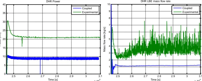
Figure 12: Power removed by the DHR (left) and LBE mass flow rate through the DHR (right).
The comparison between the LBE temperature at the inlet and outlet of the DHR is displayed in Figure 13. The calculated inlet temperature is higher than the experimental value, according to the results shown in Figure 9 (green line), while the outlet temperature is higher than the experimental one, due to the lower power removed (Figure 12 left). The discrepancy can be explained by the incorrect temperature prediction and/or incorrect modelling of the turbulence heat exchange. This aspect will be carefully analyzed in further analyses.
Figure 13: LBE temperature at inlet and outlet of the DHR.
2.5 2.6 2.7 2.8 2.9 3 3.1 x 10⁴ 0 5 10 15 20 25 30 35 40 Time [s] P o w e r [k W ] DHR Power Coupled Experimental 2.5 2.6 2.7 2.8 2.9 3 3.1 x 10⁴ 0 1 2 3 4 5 6 7 8 9 10 Time [s] M a s s f lo w r a te [ k g /s ]
DHR LBE mass flow rate
Coupled Experimental 2.5 2.6 2.7 2.8 2.9 3 3.1 x 10⁴ 180 200 220 240 260 280 300 320 340 360 Time [s] Te m p e ra tu re [ °C ] DHR LBE Temperature IN-coup IN-exp OUT-coup OUT-exp
15
4. Coupled calculations with 3D CFD model
4.1. Computational domain
Figure 14 shows the computational domain with a 3D CFD domain of the pool of CIRCE, which is the main difference with respect to the model is described in Section 3.1. In this model, the ICE test section and the DHR have the real dimensions and the correct position with respect to the pool. The grid is composed by 1450000 cells, both with tetrahedral and hexahedral elements
Figure 14: Sketch of the computational domain for 3D coupled calculations.
4.2. Isothermal test
The first coupled simulation performed with the new 3D CFD model was an isothermal experimental test in gas enhanced circulation flow. The boundary conditions of the test are reported in Table 1.
Table 1: Experimental boundary conditions of the isothermal test for gas enhanced circulation flow.
In the calculation, the argon mass flow rate is set in the RELAP5 domain, through the time dependent junction 4 (see Figure 14). The resulting LBE mass flow rate is compared with the experimental results. Figure 15 shows the comparison between the experimental trend and the input in the calculation of the argon mass flow rate. The input of the simulation was obtained as the
T[°C] FPS Power % HX Power % Gas_lift [Nl/s]
280 0 0 Step 1 1.9 Step 7 4.5 Step 2 2.3 Step 8 4.9 Step 3 2.7 Step 9 4.1 Step 4 3.1 Step 10 3.1 Step 5 3.7 Step 11 2.2 Step 6 4.1 -
-16
average of the experimental value for each step. Figure 16 and Figure 17 report the main results of this test. Figure 16 display the time trend of the LBE mass flow rate. The results are compared with the experimental values, with the RELAP5 standalone calculations and with the coupled calculations performed with the 2D CFD domain (described in [4]). Figure 17 shows the average value of the LBE mass flow rate for each step computed by the RELAP5 standalone and the coupled simulations. The numerical results are plotted as function of the experimental values. All the numerical results set within the error bands of the experimental measurements, which is 3.8% of the average value and is represented by the two dashed grey lines in the figure.
Figure 15: Time trend of the argon mass flow rate during the isothermal test
Figure 16: Time trend of the LBE mass flow rate obtained during the isothermal test.
0 0.5 1 1.5 2 2.5 3 3.5 4 4.5 5 5.5 0 1 2 3 4 5 6 7 8 x 10⁻³ Time [h] A r M a s s -Fl o w [ k g /s ] Experimetal RELAP5 0 0.5 1 1.5 2 2.5 3 3.5 4 4.5 5 5.5 40 45 50 55 60 65 70 75 Time [h] L B E m a s s f lo w [ k g /s ] Experimetal RELAP5 Coupled 2D Coupled 3D
17
Figure 17: Average values of the LBE mass flow rate during the isothermal test.
4.3. Numerical results of “Test 1” calculation
The “Test I” experiment performed in the CIRCE facility, described in Section 3.2, was simulated also using the 3D CFD domain. Due to the high CPU time required for 3D CFD simulations, this coupled calculation was restricted just to the transient stage and only the first 500 s of simulation were performed. The aim of this simulation was to analyze the differences between the 2D and 3D coupled calculations in reproducing the transition from forced to natural circulation and thermal stratification during the PLOHS+LOF accidental scenario. The initial steady-state conditions at full power and forced circulation were set independently in both the RELAP5 and CFD domains, paying attention that the conditions of pressure and LBE mass flow rate at the interfaces were corresponding. This last condition prevents the onset of instabilities. Even in this case, the power input was 95% of the nominal value in order to consider the amount of power effectively released to the LBE inside the ICE section. So, the initial power input was 693.5 kW, which is decreased to 47.5 kW at the beginning of the transient. The argon gas flow rate, the secondary water mass flow rate and the water inlet temperature are boundary conditions of the RELAP5 domain, while the air mass flow rate and the air inlet temperature are boundary conditions of the CFD domain. Moreover, the initial LBE temperature in the pool (CFD domain) was set as initial condition of the transient simulation. The temperature profile assigned to the pool followed an axial trend with a homogeneous value in each section. The axial values were assigned from the average value of the TCs measurements for each monitored section at the steady-state configuration. The same simulation was set also together with a 2D CFD in order simplify the comparison between 2D and 3D coupled calculations, since the calculation described in Section 3.4 is characterized by slightly different boundary conditions.
18
The main results of the 3D and 2D coupled simulations of the first 500 s of Test 1 are reported in the following. Figure 18 shows the LBE mass flow rate at the entrance of the FPS. The coupled calculations reproduce quite well the mass flow rate inside the test section, with a starting value of about 54 kg/s against the average experimental value of 56.7 kg/s. The transition to natural circulation flow at low power (50 kW nominal value) is well predicted up to the value of about 10 kg/s at the end of the performed simulation.
Figure 18: LBE mass flow rate in the ICE test section.
Figure 19 reports the LBE temperature at the inlet and outlet of the fuel pin simulator (left) and of the heat exchanger (right), both belonging to the RELAP5 domain. The trends are in quite agreement with the experimental data, even if the calculations predict a sudden decrease of the LBE temperature at the outlet of the heat exchanger after that the feedwater was disabled. This discrepancy could be again linked to the radial heat exchange through the shell of the heat exchanger, which is not modelled in the simulations. It can be seen in Figure 20 that in the first 100 s all the calculated power generated in the FPS is removed by the heat exchanger, while it is lower experimentally. The rate of the decrease of power removed by the heat exchanger is slower in the calculations but the final value tends toward the experimental one.
2.45 2.455 2.46 2.465 2.47 2.475 2.48 2.485 2.49 2.495 2.5 x 10⁴ 0 10 20 30 40 50 60 70 Time [s] M a s s -f lo w r a te [ k g /s ]
LBE Mass-flow rate
Experimental Coupled-2D Coupled-3D
19
Figure 19: LBE temperature across the fuel pin simulator (left) and across the heat exchanger (right).
Figure 20: Time trend of the power removed by the heat exchanger.
Figure 21 and Figure 22 report the axial profiles of the LBE temperature at the beginning of the transient (blue line), 250 s (green line) and 500 s (red line) after the beginning. Figure 21 displays the experimental results, while Figure 22 results from calculation, with the 2D CFD domain (left) and 3D CFD domain (right). LBE temperature distribution in the CFD domains of the coupled calculation is reported in Figure 23 (2D on the left and 3D on the right). As already explained in Section 3.4, in the experiment, the gradient in the upper plenum disappears once the HX is de-activated, and this behaviour is due to the radial losses through the HX. Since this phenomenon is not simulated in the coupled calculations, the gradient in the upper pool does not disappear and the flattening of the temperature profile is slower.
2.45 2.455 2.46 2.465 2.47 2.475 2.48 2.485 2.49 2.495 2.5 x 10⁴ 250 300 350 400 450 Time [s] Te m p e ra tu re [ °C ] Temperatures FPS IN-exp IN-coup-2D IN-coup-3D OUT-exp OUT-coup-2D OUT-coup-3D 2.45 2.455 2.46 2.465 2.47 2.475 2.48 2.485 2.49 2.495 2.5 x 10⁴ 200 250 300 350 400 Time [s] Te m p e ra tu re [ °C ] Temperatures SG IN-exp IN-coup-2D IN-coup-3D OUT-exp OUT-coup-2D OUT-coup-3D 2.45 2.455 2.46 2.465 2.47 2.475 2.48 2.485 2.49 2.495 2.5 x 10⁴ 0 100 200 300 400 500 600 700 800 Time [s] P o w e r [k W ] Power SG Experimental Coupled-2D Coupled-3D
20
Figure 21: Experimental profile of the axial distribution of LBE temperature in the CIRCE pool.
Figure 22: Numerical results of the axial distribution of LBE temperature in the CIRCE pool: 2D CFD domain (left) and 3D CFD domain (right).
-7000 -6000 -5000 -4000 -3000 -2000 -1000 0 250 260 270 280 290 300 310 320 330 340 350
Thermal stratification - experimental
Axial position [m] Te m p e ra tu re [ °C ] 0 s 250 s 500 s -7000 -6000 -5000 -4000 -3000 -2000 -1000 0 250 260 270 280 290 300 310 320 330 340 350 Axial position [m] Te m p e ra tu re [ °C ]
Thermal stratification - 2D coupled calculation
0 s 250 s 500 s -7000 -6000 -5000 -4000 -3000 -2000 -1000 0 250 260 270 280 290 300 310 320 330 340 350
Thermal stratification - 3D coupled calculation
Axial position [m] Te m p e ra tu re [ °C ] 0 s 250 s 500 s
21
Figure 23: LBE temperature distribution inside the CIRCE pool, 2D domain on the left and 3D domain on the right.
The results about the operation of the decay heat removal system are reported from Figure 24 to Figure 26. Figure 24 shows the air mass flow rate (left), which is set as boundary condition, the difference between outlet and inlet temperatures across the DHR on the right. The numerical results underestimate considerably the DHR efficiency. It can be noticed from the air temperature difference across the DHR, form the total power removed by the heat exchanger (Figure 25 left) and from the LBE mass flow rate inside the DHR shell (Figure 25 right). Consequently the decrease of the LBE outlet temperature is much slower in the calculations with respect to the experiment (in Figure 26).
Figure 24: Air mass flow rate (left) and air temperature difference across the DHR (right).
2.465 2.47 2.475 2.48 2.485 2.49 2.495 2.5 x 10⁴ 0 50 100 150 200 250 300 Time [s] A ir M a s s f lo w r a te [ g /s ]
DHR Air Mass-flow rate
Experimental Coupled-2D Coupled-3D 2.465 2.47 2.475 2.48 2.485 2.49 2.495 2.5 x 10⁴ 0 20 40 60 80 100 120 140 160 180 Time [s] Te m p e ra tu re [ °C ] T air DHR Experimental Coupled-2D Coupled-3D
22
Figure 25: Power removed by the DHR (left) and LBE mass flow rate through the DHR (right).
Figure 26: LBE temperature at across the DHR.
In spite of a good qualitative comparison between the numerical results and the experiment, concerning the main thermal-hydraulic parameters of DHR system, a quantitative discrepancy can be noticed. This gap was explained a posteriori with an inadequate simulation of the turbulent heat transfer. In natural circulation regime, the efficiency of the heat exchanger affects also the hydraulic head and so the LBE mass flow rate. Moreover, some differences are observed also between the 2D and 3D calculations. Being the boundary conditions the same in both the simulations, this discrepancy seems to be more related to the difference in pressure drops, such as the ones at DHR inlet. As show in Figure 27, the slots for the LBE entrance are represented accurately in the 3D model, while is modeled through an equivalent opening in the 2D domain. Nevertheless, all these aspects need to be still carefully analyzed in order to confirm the hypotheses and then improves the modeling of the pool system.
2.465 2.47 2.475 2.48 2.485 2.49 2.495 2.5 x 10⁴ 0 5 10 15 20 25 30 35 40 Time [s] P o w e r [k W ] DHR Power Experimental Coupled-2D Coupled-3D 2.45 2.455 2.46 2.465 2.47 2.475 2.48 2.485 2.49 2.495 2.5 x 10⁴ 0 1 2 3 4 5 6 7 8 9 10 Time [s] M a s s f lo w r a te [ k g /s ]
DHR LBE mass flow rate
Experimental Coupled-2D Coupled-3D 2.45 2.455 2.46 2.465 2.47 2.475 2.48 2.485 2.49 2.495 2.5 x 10⁴ 180 200 220 240 260 280 300 320 340 360 Time [s] Te m p e ra tu re [ °C ] DHR LBE Temperature IN-exp IN-coup-2D IN-coup-3D OUT-exp OUT-coup-2D OUT-coup-3D
23
Figure 27: LBE inlet in the DHR for the 2D domain (right) and the 3D domain (left).
5. CIRCE-HERO model for coupled calculations
The CIRCE-HERO configuration consists in the installation of the test section HERO inside the CIRCE facility. The remaining part of the primary system is the same described in [5]. HERO is a heat exchanger made of seven double wall bayonet tubes enclosed in a hexagonal shell. It represents, as much as possible, the ALFRED SG tubes (1:1 in length). A complete description of the CIRCE-HERO facility can be found in [7], while Figure 28 shows a sketch of the CIRCE facility with the HERO test section.
24
5.1. RELAP5 3.3 nodalization of CIRCE-HERO
A preliminary RELAP5 nodalization of CIRCE-HERO have been modeled and described in [7]. It is composed by 11 macro-regions: five of them are devoted to modeling of the pool, four parts model the entire test section (included the LBE side of HERO), then the water side of HERO and the air side of the DHR. Figure 29 shows a scheme of the nodalization and some relevant parts are highlighted. This nodalization was employed to perform preliminary RELAP5 standalone calculations on CIRCE-HERO. Nevertheless, this nodalization is not definitive and some work is still ongoing in order to finalize it.
Figure 29: RELAP5 3.3 nodalization of CIRCE-HERO
5.2. Geometrical domain for CIRCE-HERO coupled calculations
The ongoing work is finalized to perform coupled calculations of CIRCE-HERO. For this purpose, the RELAP5 nodalization needs to be modified. In particular, the part that models the test section (FPS, riser, separator HERO) and the secondary side of the heat exchanger will be simulated by RELAP5. Similarly, to the procedure adopted to simulate the ICE configuration, the pool and the DHR will be modeled with the CFD code. Figure 30 displays the computational domain foreseen for the RELAP5-ANSYS Fluent coupled calculations. The coupling procedure is the same adopted for previous calculations in a pool system (see Section 3.1), so are the exchanged data (see Figure 4). Regarding the modeling of the pool, the geometrical domain and the main dimensions have been already completed. More analyses are focusing on the spatial discretization. The objective is to reach a good compromise between accuracy and CPU time required for the calculation, which is the main drawback of the 3D modeling. Figure 31 shows one of the grid obtained, which is a non-conformal mesh characterized by both tetrahedral a hexahedral elements. The domain was divided
ICE inlet 0.000 Branch 190 -0.350 3 1 p ip e 2 0 sngljun25 0.300 sngljun35 0.700 4 p ip e 3 0 1 2 1 pipe40 0.970 sngljun45 p ip e 5 0 11 1 3 1 pipe 6 0 sngljun55 2.560 3.010 branch65 3.160 3 p ip e 7 0 1 3.750 branch91 branch90 p ip e 1 0 0 1 25 3.460 tmdvol 80 – Ar in tmdjun85 7.210 branch104 branch 107 tmdvol 999 Ar out 7.388 7.688 7.838 Cover Gas branch108 8.088 branch 111 branch110 branch109 3.910 p ip e 1 2 0 22 1 p ip e 1 2 2 22 1 1 p ip e 1 2 1 22 p ip e 1 1 4 22 1 mp jun mp jun p ip e 1 1 5 25 1 branch 130 branch 131 branch 132 mp jun mp jun 1 2 pipe150 1 2 pipe151 1 2 pipe152 sngjun153 mp jun mp jun
branch155mpbranch156 branch157
jun mp jun 1 3 pipe160 1 3 pipe161 1 3 pipe162 mp jun mp jun
branch170 branch171 branch172
2.410
7
pipe175 7pipe176 7pipe177
mp jun mp jun 1 1 1 1.435 mp jun mp jun
branch180mpbranch181 branch182
jun mp jun p ip e 1 8 5 1 11 p ip e 1 8 6 1 11 p ip e 1 8 7 1 11 1.260 mp jun mp jun 7.538 p ip e 2 4 0 1 2 41 9 49 41 1 tmdvol 250 Water in 8.798 1 sngljun275 tmdjun255 p ip e 2 7 0 p ip e 2 8 0 48 branch285 tmdvol 290 steam out tmdvol 305 air in tmdjun310 8.788 B r a n c h 3 1 5 p ip e 3 2 0 1 26 branch 325 p ip e 3 3 0 26 1 B r a n c h 3 4 0 tmdvol 350 air out sngjun345 separatr 105 branch 238 branch 239 HERO (1 tube) secondary side
ICE-HERO test section DHR-air side
DHR-LBE side
25
into many parts with the aim to maximize the use of hexahedral meshes. Approximately, a satisfactory grid is composed by about 2.4M cells and 1.2M nodes.
Figure 30: Computational domain of the CIRCE-HERO facility for coupled calculations.
Figure 31: Spatial discretization of the new 3D CFD domain, for the CIRCE-HERO calculations.
3 1 p ip e 2 0 sngljun25 4 p ip e 3 0 1 2 1 pipe40 p ip e 5 0 11 1 3 1 pip e 6 0 branch65 3 p ip e 7 0 1 branch91 branch90 p ip e 1 0 0 1 25 tmdvol 80 – Ar in tmdjun85 branch104 tmdvol 999 Ar out p ip e 2 4 0 1 2 41 9 49 41 1 tmdvol 250 Water in 1 sngljun275 tmdjun255 p ip e 2 7 0 p ip e 2 8 0 48 branch285 tmdvol 290 steam out separatr 105 branch 238 branch 239 TDV-10 TDV-250 T2 ṁ1 ṁ2 P2
26
6. Conclusions
The present work focuses on the application of a coupling methodology between CFD codes and thermal-hydraulic system codes to the pool-type facility CIRCE. The analysis was performed using the coupling methodology developed and improved in the past years at the “Dipartimento di Ingegneria Civile e Industriale” of University of Pisa.
The coupled calculation of a PLOHS+LOF accidental scenario inside CIRCE facility was accomplished and the main results were compared with the experimental data. In the coupled calculations, the CFD domain includes just the modeling of the pool, with the aim to predict the thermal stratification phenomena occurring in the pool during an accidental scenario. A first calculation was performed with a 2D axis-symmetric domain of the pool region. The calculation allows representing more accurately the boundary conditions of the test and the phenomena involved during the transient with respect to the CFD and RELAP5 standalone simulations, with a qualitative agreement of the numerical results with the experimental data. Nevertheless, there are still some quantitative discrepancies, mainly due to some simplifications in the modeling. The outcome of this analysis will be taken into account to improve the model for the future simulations. A 3D CFD model of the pool was also developed, which allows to eliminate the inaccuracy related to the non-realistic axial-symmetric hypothesis and to analyze 3D phenomena. On the other hand, the 3D model requires a spatial discretization with higher number of cells, so it requires a longer CPU time. The 3D model was used also to simulate the first part of a PLOHS+LOF transient and to compare the results with an analogous computation performed using a 2D CFD domain. The main numerical results showed a good qualitative prediction of the phenomena occurring during the transient, with some quantitative discrepancies in the representation of the DHR system due to an inadequate modeling of the turbulent flow. Some differences are also detected between the 2D and 3D simulations, more likely due to the geometrical simplifications of the 2D modeling. Further work is still going on with the aim to find the best way to simulate the pool system CIRCE, saving as much as possible the computational time but preserving the adequate accuracy.
The lesson learned from the previous analyses has been helpful in the development of the model for the new experimental test section HERO, which is installed inside the CIRCE pool. A preliminary RELAP5 nodalization of CIRCE-HERO was developed, but some work is still ongoing to finalize it. Moreover, this model will be modified and adapted for the coupled calculations. In the meanwhile, a 3D CFD model of the pool have been built, with a focus on the spatial discretization, with the aim to reach a compromise between accuracy of the calculations and CPU time required. The future efforts are addressed to complete the modeling of both the RELAP5 and CFD domains and to apply the coupling tool to the facility CIRCE-HERO in order to analyze the performance of the new test section.
27
Nomenclature
Abbreviations and acronyms
AdP Accordo di Programma
CFD Computational Fluid Dynamic
CIRCE CIRCulation Experiment
CORBA Common Object Request Broker Architecture
CPU Central Process Unit
DHR Decay Heat Removal
DICI Dipartimento di Ingegneria Civile e Industriale
ENEA Agenzia nazionale per le nuove tecnologie, l’energia e lo sviluppo sostenibile
FPS Fuel Pin Simulator
HERO Heavy liquid mEtal pRessurized water cOoled tubes
HS Heat Source
HX Heat Exchanger
ICE Integral Circulation Experiment
LBE Lead bismuth eutectic
LOF Loss of Flow
NACIE Natural Circulation Experiment
PLOHS Protected Loss of Heat Sink
RELAP Reactor Loss of Coolant Analysis Program
STH System Thermal Hydraulic
TUI Text User Interface
UDF User Defined Function
28
References
[1] D. Martelli, N. Forgione, G. Barone e A. Del Nevo, «Pre-test analysis of thermal-hydraulic behaviour of the NACIE facility for the characterization of a fuel pin bundle,» Adp MSE-ENEA
LP3-C4, 2012.
[2] D. Martelli, N. Forgione, G. Barone e W. Ambrosini, «System codes and CFD codes applied to loop-and pool-type experimental facility,» Adp MSE-ENEA LP2.C1, 2013.
[3] D. Martelli, N. Forgione, G. Barone e W. Ambrosini, «Validation of the coupled calculation between RELAP5 STH code and Ansys Fluent CFD code,» Adp MSE-ENEA LP2.C1, 2014. [4] F. Andreoli, G. Damiani, D. Martelli, N. Forgione, W. Ambrosini, « Preliminary verification
and validation of coupled calculation between the RELAP5/Mod. 3.3 STH code and the CFD code ANSYS Fluent » Adp MSE-ENEA LP2.C1, 2015.
[5] G. Bandini, I. Di Piazza, A. Del Nevo, M. Tarantino and P. Gaggini, “CIRCE experimental set-up design and test matrix definition,” ENEA UTIS-TIC Technical Report, IT-F-S-001, 28 02 2011.
[6] N. Forgione, D. Martelli, W. Ambrosini and F. Oriolo, "Final report on qualification of CFD modelling approaches," THINS-Deliverable, D-N: 2.1.10, 19/02/2015.
[7] D. Rozzia, A. Del Nevo, N. Forgione, "CIRCE Pre-Test calculation report", MYRTE-Milestone