FEMLCORE-CATHARE coupling on Salome platform

(1)

(2)

(3)

FEMLCORE–CATHARE coupling on

SALOME platform

A. Attavino, D. Cerroni, A. Cervone, L. Fancellu,

and S. Manservisi

(4)

Introduction

A nuclear plant is a very complex machine and its numerical simulation is nowadays above the power computability of the actual computers. A complete study of this ma-chine is multi-physics and multiscale and every detailed engineering study should be lim-ited to well defined regions and a single-physical phenomenon. If the three-dimensional effects are ignored the components of the nuclear plant can be modeled by simple volu-metric balances of energy, momentum and mass. The 0-dimension components can be connected with simple mono-dimensional pipes. The mono-dimensional pipes describe the evolution of the state fields interacting with the external environment by adding external sources in the mono-dimensional conservation equations. The Cathare code and other system codes were developed based on this simple hypotheses [5, 6]. These codes have been developed long time ago and during this period has been continuously updated and verified with many experiments [2, 5].

In many situations the mono-dimensional model cannot explain how the system evolves since bi or three-dimensional effects are important. However the three-dimensional sim-ulation of large o complex parts of the system are not possible. In fact nowadays one can simulate only small parts of the nuclear reactor when realistic boundary conditions are available. The coupling techniques between system codes, which may give appropri-ate boundary conditions, and three-dimensional simulation gives a good opportunity to explore more complex problems.

In early reports we have developed FemLCore code to simulate three-dimensional nuclear reactor components such as the core the upper and the lower plenum. In the previous report we have simulate the the core with a 3D-porous FemLCore module, the plena with a 3D-CFD FemLCore module and the primary loop with a 1D-libMesh or 1D-CFD FemLCore module. In order to improve the quality of the coupling it is very interesting to couple 3D-porous FemLCore module with a mono-dimensional system code that contains trusty information about nuclear power plant such as the Cathare code. It is even more interesting to explore the coupling where the three-dimensional simulations are added as a correction to the mono-dimensional system simulation so that one can evaluate the need of the use of these expensive CFD computations.

In this report we developed a coupling algorithm on the Salome platform between the FemLCore and Cathare code where the numerical approach is a defective correc-tion approach. This means that we solve the Cathare problem over all the domain overlapping partially this mono-dimensional mesh to the three-dimensional one where the solution is obtained with FemLCore module. The mono-dimensional system is al-ways solved generating the boundary conditions for the CFD three-dimensional code and then the three-dimensional solution gives back corrections in the form of sources in the conservation equations to the Cathare code.

(7)

Great difficulties arise from the complexity of combining the three and the mono-dimensional mesh together. The input-output formats for mesh and solutions should be compatible. Data should be exchanged at each time step. The Salome platform gives the help needed since an interface compatible with this platform has been developed by the Cathare research group. The Cathare code is not open source and therefore without data transfer functions would be impossible to get and set data inside the code.

Chapter 1 is devoted to the description of the implementation of the Cathare coupling class. There are two classes that can be used to transfer data from Cathare code to the Salome platform: the ICoCo package and the Problem_Cathare interface developed in this report. The ICoCo interface is provided with the Cathare code and uses the

TriouField format to exchange data with Salome platform. In this work we use a modified

version of the Problem_Cathare interface which is equipped with graphical class which allows the the evolution of the fields time by time. In this class the transfer with the Salome platform is based on simple c++ double type format.

In Chapter 2 there is a brief description of the implementation of the FemLCore coupling class. In this Chapter we point out the main functions to be used inside the supervisor. Details on volume and surface interfaces are introduced. The cmake file for the compilation of the FemLCore and Cathare coupling classes is briefly described.

Chapter 3 starts with a brief description of a standard project of a user application of the type FemLCore-Cathare. Two coupling tests are presented. Test 1 is performed with a simple three-dimensional core model reactor coupled with the primary mono-dimensional loop which consists of a pump and a heat exchanger. In Test 2 a more realistic three-dimensional reactor with core and lower and upper plenum is coupled with a primary mono-dimensional loop. Details on Cathare and FemLCore meshes and on the supervisor code are shown.

(8)

1 Cathare on Salome Platform

1.1 Cathare MESH on Salome

Cathare code is a system code essentially capable of computations over mono-dimensional meshes. The mesh is read by Cathare through a text parser which uses its own library commands. This mesh for mono-dimensional computations consists of several groups of directives that defines geometric modules. It can be generated by using the GUI interface on SALOME platform called GUITHARE.

Figure 1.1: GUITHARE main window on Salome 5.

1.1.1 GUITHARE installation

The graphical mesh generator GUITHARE is a GUI written by CEA and EDF, dis-tributed under different forms of licenses. The package is disdis-tributed in binary form for different Linux distributions. In this report we use the open SUSE 13.2 (Harlequin)

(x86_64) and therefore the appropriate package is the GUITHARE_V1.8.5_SUSE9_64bit_20130703.tar.gz. The installation of this binary package presents many problems since the libraries used

for the interface GUITHARE are not updated for recent Linux distributions. After performing the untar command of this package the scripts

(9)

appear in the main directory. They cannot run in this original form since they are written with dos editors. It is necessary to apply the dos2unix command to both files to delete the dos end line control characters. The command for run.csh is

dos2unix run.csh .

Now the script run.csh can run under the following Linux command ./run.csh .

The script cannot open the GUI and an error appears as

error while loading shared libraries: libstdc++.so.5:

cannot open shared object file: No such file or directory.

The library libstdc++ is the standard C++ library, needed for dynamically linked C++ programs. The version libstdc++.so.5 is rather old and now the libstdc++.so.6 is installed in the OpenSuse 13.2 distribution. In order to install the old library

lib-stdc++.so.5 one can go to OpenSuse web page. Select libstdc++33, the standard C++

shared library, and select the option Click Install on 64 Bit:

devel:gcc 3.3.3 32 Bit 64 Bit 1 Click Install .

The old library libstdc++.so.5 is now installed on the OpenSuse 13.2 distribution. Even now the script cannot open the GUI and the new following error reads

error while loading shared libraries: libpng.so.3:

cannot open shared object file: No such file or directory.

The libpng.so.3 is an old version of the png package so that in the OpenSuse 13.2 is now installed the library libpng16.so.16.13.0. The libraries are not compatible. The library

libpng12.so is compatible with libpng.so.3. By using yast2 the library libpng12 can be

installed and linked properly. The following link commands should be executed

ln -s /usr/lib64/libpng12.so /usr/lib64/libpng.so.3 .

Now a new error appears as

cannot load library libCathareGUI.so:

libexpat.so.0 cannot load shared object file

In the OpenSuse 13.2 is now installed the libexpat1.so. The libexpat0.so can be installed by using yast2 together with libexpat1.so in this Linux distribution.

(10)

Figure 1.2: Cathare main hydraulic modules.

1.1.2 Cathare modular structure

Information on Cathare code can be found on the Cathare documentation [1, 2, 3, 5, 6, 7]. In the Cathare code several main modules are assembled to model sub-component circuits.

Different circuits can be connected to assemble the main plant circuit (reactor0). The main modules in Cathare are four: AXIAL, VOLUME, THREED and BCONDIT. They can be added to the circuit (called CIRCUIT0) by selecting, in the GUITHARE main window, the add custom hydraulic module under CIRCUIT on the right mouse button menu as shown in Figure 1.2. An AXIAL module is a mono-dimensional module needed to describe components such as pipes. This module is shown in Figure 1.3. It is defined by two points called junctions (J1 and J2). On the line between the two junctions a mesh with sub-meshes is constructed. The point partition is defined in the XAXIS panel. In Figure 1.3 the mesh consists of two points: AXI11 and AXI12. Points can be added or deleted with the + or − button. The points define an interval which can be discretized in Nb meshes defined in the MESH panel. In this panel one can define the direction by setting the cos cell. By putting 0,1, -1 in the cos cell the line is horizontal, upward vertical or downward vertical respectively. In the GEOMETRY panel the section and the dimension of the pipe can be controlled. The corresponding command code generated by GUITHARE are as following

AXIAL = AXIAL J1 USTREAM J2 DSTREAM ; AXIAL11 = XAXIS 0. ;

AXIAL12 = XAXIS 1. ; LAXIA1 = AXIAL11

(11)

Figure 1.3: Cathare AXIAL hydraulic module. MESH AXIAL LAXIA1;

GEOM AXIAL (AXIAL11 AND AXIAL12) SECT 0.785398 PERI 3.1415926 SIZE 1.;

This code defines the AXIAL geometric module. The semicolon ends the definition. There are only two points (AXIAL11,AXIAL12) at the mono-dimensional coordinate

x = 0 and x = 1 with one SEGMENT divided into 10 elements in the horizontal

direction (cos 0).

A volume module is a zero-dimensional module, which consists of a two-node module used to describe large size plena with several connections, such as pressurizers, steam generator domes and upper and lower plena. The volume module is shown in Figure 1.4. The corresponding code is as follows [3]

VOL1 = VOLUME J3 DSTREAM J4 DSTREAM J5 DSTREAM ; GEOM VOL1

0. 1. .5 1.

J3 TOP LENGTH .1

SECT 0.007853981633 PERI 0.314159265 SIZE .1 VERTICAL J4 BOTTOM LENGTH .1

SECT 0.007853981633 PERI 0.314159265 SIZE .1 VERTICAL J5 BOTTOM LENGTH .1

(12)

Figure 1.4: Cathare VOLUME hydraulic module.

In VOL1 of Figure 1.4 two nodes and three junctions (J3,J4,J5) are defined in the vol-ume and junction panels respectively. For each junctions the geometrical configuration should be defined in the appropriate panel. The junctions can enter into the VOLUME horizontally or vertically as specified in the junctions parameter panel of the VOLUME module. The BC boundary condition module is used to model the boundary conditions defined by the external components of the reactor or external facilities. Different bound-ary conditions can be specified. BCONDIT modules may be of two types: internal or external type. In internal type modules variables are defined with respect to time (with the ABTIME directive). In the external type modules variables are not time-dependent but imposed externally (and explicitly) by the user via the input deck. There are three kinds of boundary conditions: inlet, outlet and mixed boundary conditions. For details see [1, 2, 5, 6] The BCONDIT module is shown in Figure 1.5. In this Figure a BC3B (internal) boundary condition model is selected. For this boundary conditions an inter-val of time (REALLIST 0. 100.) must be defined where the state variables should be specified on the boundary. In this case liquid temperature TL is set to (20-20) in the time interval defined by the ABTIME directive. In this case the temperature is fixed to 20C during the whole interval of time. In the same way the gas temperature TG and the velocity VL and VG are to be specified. The corresponding code generates by GUITHARE is written as [3, 5]

BC = BCONDIT J1 DSTREAM ; MODEL BC BC3B

(13)

Figure 1.5: Cathare BCONDIT hydraulic module. TG (REALLIST 100100. )

ALFA (REALLIST 1.E-5. 1.E-5. ) VL (REALLIST 0.1 0.1 )

VV (REALLIST 0.1 0.1 )

ABSTIME (REALLIST 0. 100. );

The THREED module attempts to describe multidimensional effects in a vessel. Together with module there are modules that are selected in an appropriate sub-menus. Each module can have sub-modules. Some popular sub-modules are the TEE and the HEAT EXCHANGER sub-module The TEE sub-module is used to represent a lateral branch (tee-branch) on a 1D module. Heat exchanger sub-modules can be used between two circuits or between two elements of a circuit [3, 5].

1.2 The Cathare coupling interface on Salome

There is a coupling interface created by the Cathare team. The interface is obtained by creating a c++ wrapper for input and output of the Cathare variables. We simplify this class to obtain a very light a friendly interface on Salome platform. The original wrapper class is called ICoCo. For details see [1, 2, 5, 6, 7]. The ICoCo wrapper and a new lighter one, defined through the c++ class Cathare_problem are actually present at the same time in this code. The ICoCo wrapper is compiled in the library libCathare.so while the class Cathare_problem can be used as standard class and compiled together with the main function main.cpp (called supervisor). In summary there are two classes that can be used to transfer data from Cathare code to the Salome platform: the ICoCo package and the Problem_Cathare interface developed in this report.

(14)

1.2.1 The ICoCo supervisor

The compilation and linking of the ICoCo supervisor is not a standard procedure and everything needed for this purpose is written in the Makefile_gad included in the ICoCo package. First Cathare and the ICoCo wrapper should be compiled with the environment key $v25_3 set to the Cathare code main directory (. . . /Cathare2/v25_3/mod2.1/). Then one uses the input deck Cathare file *.dat, creates the final library libCathare_gad.so, uses main.cpp and creates the executable superv with the command

DATAFILE=omega.dat make -f $v25_3/ICoCo/Makefile_gad .

A datafile used with ICoCo must have certain features in order to be parsed and to allow the control of the time loop by an outside supervisor. The exec block should have a standard look

(...) <- may include steady state loop

REPEAT BLOCKnn nnn; <- should be outermost loop (...)

TIME = TIME + DT;

TRANSIENT CIRCTOT TIME DT; DT = NEWDT;

TIME = NEWTIME; (...)

IF ( TIME>TMAX ); <- will be ignored in the supervisor QUIT BLOCKnn ;

ENDIF (...)

END BLOCKnn ; (...)

The supervisor is the C++ file main.cpp. The main.cpp should be written with modular functions and should be easy to read and reuse. The supervisor can be run with the command

./superv For details see [7].

1.2.2 The Problem_Cathare interface

We are not going to use the ICoCo package but mainly the Problem_Cathare interface. This interface consists of four basic files with its corresponding headers: CathareM,

problem_Cathare, SaveCatDataM and axial_io.

The CathareM.cpp and CathareM.h files contain the c++ wrapping of the FORTRAN main Cathare files. The main functions are

(15)

bool ecrire(double value, std::string keyword,

std::string cname, int imesh, int irad); bool ecriri(int value, std::string keyword,

std::string cname, int imesh, int irad); double value(std::string keyword, std::string cname,

int imesh, int irad, int& ivstat); bool parse_name(std::string name, std::string& keyword,

std::string& cname, int& imesh, int& irad);

The ecrire and ecriri functions write the double or the int variable in the Cathare codes. The variable is defined by four arguments: std::string keyword (variable name),

std::string cname(module name), int imesh (mesh element) and int irad (angle value).

The parse_name function is a function that parses the name into the four argument

keyword, cname, imesh and irad. For example if name=PRESSURE_AXIAL1_10

then keyword=PRESSURE, cname=AXIAL1 and imesh=10. The irad is automatically set to 0. The ICoCo library uses the functions through the single name argument while the new Problem_Cathare class directly by four split arguments.

The Problem_Cathare class is the core of the coupling. The main functions of the

Problem_Cathare class are shown in Table 1.1. We remark that the function

getValue_Cathare(string keyword,string cname,int ix, int irad, double val) and

setValue_Cathare(string keyword,string cname,int ix, int irad)

are not contained in the ICoCo interface. The setValue_Cathare function has four input arguments: keyword, cname, imesh and irad. The getValue_Cathare function has the four previous mentioned input arguments and one output argument: the output variable is the value read from Cathare. The TrioField variable type is not present in this class while it is the standard type for exchange variable in ICoCo interface. The exchange between the Cathare code and the supervisor is done by using simple double type variables.

Cathare code needs to store and retrieve data. In FORTRAN programs the data are inside the common block data. The SaveCatData is the structure used for sav-ing/restoring the FORTRAN commons (Cathare and Pilot) by using the functions in the SaveProblemData class. This class saves only the used portion of the commons and the variables of a Problem_Cathare itself. The data structure SaveCatData is described in the Table 1.2 where the FORTRAN commons and all the possible variables of a Prob-lem are written. SaveCatData class consists of two main functions: save and restore function as shown in Table 1.3.

The Problem_Cathare interface includes also the files axial.cpp and axial.h, that in-clude the class that allows to print in XDMF format. In this way the Cathare solution

(16)

return type function

start/stop program

bool initialize()

void terminate()

void setDataFile(·);

interface time step

double presentTime() const;

double computeTimeStep(·) const;

bool initTimeStep(·);

bool solveTimeStep();

void validateTimeStep();

bool isStationary() const;

void abortTimeStep();

interface saving

void save(·,·) const;

void forget(·,·) const;

void restore(·,·,·);

interface FieldIO

vector< string > getInputFieldsNames() const;

void getInputFieldTemplate(·,·,·,·) const;

void setInputField(·,·);

vector< string > getOutputFieldsNames() const;

void getOutputField(·,·) const;

Problem_Cathare class only interface FieldIO

double getValue_Cathare (·,·,·,·)

void setValue_Cathare (·,·,·,·,·)

Table 1.1: Problem_Cathare class.

can be seen at any time together with the three-dimensional one on the Paraview visual-izer. The variables that should be printed and visualized for each axial are defined in a vector of strings: the varNames vector. For example if one would like to see the values of the Cathare variables ALFA, GASTEMP, LIQFLOW, LIQH, LIQTEMP, PRESSURE, LIQV one must define the static vector at the top of the file axial.cpp as

const static std::vector<std::string> varNames= { "ALFA", "GASTEMP", "LIQFLOW", "LIQH", "LIQTEMP", "PRESSURE", "LIQV"

(17)

return function description void fill_sizes();

void save_Cathare() save Cathare commons

void save_Pilot(); save here the Pilot commons

void restore_Cathare(); restore from here the Cathare commons void restore_Pilot(); restore from here the Pilot commons

int Cathare_dsize;

double* Cathare_doubles; int Cathare_isize;

int* Cathare_ints; COMMON DIMENSION

int Cathare_csize; char* Cathare_chars; int Cathare_psize; void** Cathare_pointers; int Pilot_dsize; double* Pilot_doubles; int Pilot_isize; int* Pilot_ints;

Table 1.2: SaveCatData class is the structure used to contain the data commons and the variables of a Problem_Cathare.

return function description

void save (const Problem_Cathare& what) save data void restore (Problem_Cathare& where) restore data

Table 1.3: SaveCatData class functions to extract and store Cathare variables. };

Each axial is defined by using the structure AxialData as reported in Table 1.4. The

type data description

string name; component name

int nCells; total number of elements

vector<double> blockCoord; coordinates

vector<uint> blockN; elments in each block vector<double> cos; directions

Table 1.4: Axial data structure.

Axial class contains an AxialData class structure (called _data) a Problem_Cathare class

(18)

the axial data as in Table 1.4 while the Problem_Cathare class pointer allows the data exchange with a FORTRAN code itself. The boolean flag _writeFlag set the print in XDMF-HDF5 or VTK format for Paraview visualization [36, 32]. The functions of the

Axial class are defined in Table 1.5. For each AXIAL the Axial class reads from the

type function

void setName( const std::string name)

void setNNodes(const int nCells )

void write(double const time,int const step)

vector<vector<double> > _getData();

void _writeHDF5Sequence(·,·,·);

void writeXDMF(·, ·);

void writeHDF5(·, ·);

void writeHDF5mesh() const;

void writeVTK(·, ·);

void writeVTKSequence();

Table 1.5: Axial class functions.

input Cathare deck file its data and fill Axialdata vector. With reference to the following portion of code

AXIAL1 = AXIAL1 J1 USTREAM J2 DSTREAM ; AXIAL11 = XAXIS 0. ;

AXIAL12 = XAXIS 1. ; LAXIA1 = AXIAL11

SEGMENT 10 AXIAL12 COS 0. ; MESH AXIAL1 LAXIA1;

GEOM AXIAL1 (AXIAL11 AND AXIAL12) SECT 0.785398 PERI 3.1415926 SIZE 1.;

in the Axialdata vector we have the module name name=AXIAL1, the total number of elements nCells=10, the coordinate vector blockCoord=0,0,0,1, elements in each block blockN=10; direction vector cos=0.

1.3 Cathare post-processing on Salome

There are three ways to see the Cathare results on Salome: the standard Cathare text output, the graphical GUITHARE and on the Salome platform by using Paraview with XDMF-HDF5 format [36, 32, 4].

1.3.1 Cathare text output

The post-processing of the results can use the graphic input data deck and the binary file FORT21 to display the data. The post-processing of results is performed afterward

(19)

by postpro.unix. The command has the following format postpro.unix test-caseg.dat

where test-caseg.dat is the name of the input deck file. The postpro.exe reads the file DICO and generates the ASCII evolution file FORT07 from the result file FORT21 on the basis of user selected variables [1, 2, 4]. If one wants to create and use a local

postpro.exe instead of the standard one, one must add the second argument Âń mask

Âż in postpro.unix procedure used.

1.3.2 GUITHARE with FORT21 output file

Figure 1.6: GUITHARE import result window.

Post-processing can use a graphic input data deck and the binary file FORT21. In Figure 1.6 the FORT21 is loaded by using the menu of the exec menu. The GUITHARE graphical mode is then activated, as in Figure 1.7, and finally the graph is displayed (Figure 1.8) [4].

1.3.3 Paraview XDMF-HDF5

The new Problem_Cathare class generates the mesh file AXIAL_mesh.h5 that con-tains the coordinates and the connectivity structure. Also the AXIAL.time.h5 and its driver in XDMF format AXIAL.time.xmf are generated. The file in XDMF format

AXIAL.time.FEMuS can be opened by using the Paraview application as shown in

Fig-ure 1.9 [36, 32]. The great advantage of this approach is that the solution fields can be seen during the evolution and not only at the end of the computations.

(20)

Figure 1.7: GUITHARE graphical mode button.

(21)

(22)

2 Implementation of FemLCore on Salome

Platform

2.1 SALOME-FemLCore interface

FEMuS SRC INCLUDE USER_APPL ... ... FEMUS.h Mesh Extended.h Function.h Interface Interface Function.h Mesh Extended.h FemLCore EquationSys Extended.h EquationSys Extended.h FEMUS.h

Figure 2.1: Diagram of the FEMuS interface class to the Salome Platform. The FemLCore code implement modules aimed at computation of 3D core thermal-hydraulics of fast nuclear reactors [13, 14, 15, 16]. As shown in Figure 2.1 the FEMuS interface to the Salome platform is organized in four files or classes: FEMuS,

Equation-SystemsExtendedM, ParallelMeshExtendedM and LibMeshFunctionM. All these classes

are located in the src FEMuS directories. The corresponding headers are located in the include FEMuS directory. The FEMuS interface allows to pass commands from MEDMem library to the EquationSystemsExtendedM class which is the problem solver function and viceversa [17, 18, 19]. The FEMuS class is a c++ class that can

(23)

com-Type name data description

MGFEMuSInit * _start; start function

MPI_Comm _comm; communicator

bool _local_MPI_Init initial mpi flag

MGUtils * _mg_utils param and files

MGFEMap * _mg_femap fem map

MeshExtended* _mg_mesh FEMuS-mesh

MEDCouplingUMesh * _med_mesh Med-mesh

EquationSystemsExtendedM* _mg_equations_map system

MGTimeLoop * _mg_time_loop transient

Table 2.1: FEMuS data structure.

Type name data description

FEMUS() constructor

void terminate() end

void init_param(·) init param

void init_fem(·) init fem

void setMesh() set mesh

void setSystem(·,·,·) set system

const MeshExtended & get_MGMesh() get GMesh

const EquationSystExtM& get_MGExtSystem() get system

void solve_setup(·,·) initial setup

void solve_onestep(·,·,·,·,·) transient

void solve_non_linear_onestep(·,·,·,·,·) transient

void solve_control_onestep(·,·,·,·,·) one time step

Table 2.2: FEMuS interface functions to FemLCore code.

municate data into and from the FemLCore code. It contains data and functions that are show in Table 2.1 and Table 2.3. In Table 2.1 there is the list of data, mainly pointers needed to transfer data from one mesh format to another, namely MGMesh to MED format. The pointers _mg_mesh and _med_mesh refer to the mesh in their respective MGMesh and MED format. The FEMuS class needs information to extract data from these different mesh structures. In particular, the classes MGUtils,

MGGe-omEL, MGFEMap and MGFemusinit must be available inside the FEMUS interface to

transfer basic information such as file names, parameters, multigrid level, fem elements, etc. The MGUtils contains all the file names and input parameter values. The

MGGe-omEL and MGFEMap contain information about the finite element mesh structure and MGFemusinit class is the manager class for MPI and multigrid solvers [18, 19].

The FEMuS class contains the FemLCore commands and the SALOME platform data structure. Each code interface implemented on Salome platform must have similar

(24)

Type name data description

void setMedMesh(·) set Med mesh

void init_interface(·,·,·,·,·,·) init interface

void init_interface(·,·,·,·,·,·,·) init interface

void setAnalyticSource(·,·,·) set anal field

void setFieldSource(·,·,·) set num field

void write_Boundary_value(·,·,·,·,·) set bd value

void setAnalyticBoundaryValues(·,·,·) set anal bd value

double getAvOnBoundary_nodes(·,·,·) get av

MEDCouplingFieldDouble * getValuesOnBoundary(·,·,·,·) get field Table 2.3: FEMuS interface functions to Salome platform.

commands to run the code from the same supervisor program main.cpp. As shown in Ta-ble 2.2 the functions that start and stop the code are the constructor FEMUS(MPI_Comm

comm) and the function terminate(). These functions take into account the start and

stop of all MPI parallel processes of the code. The initialization of the parameters and the FEM elements for the FemLCore project are obtained by the following functions void init_param(MGUtils &mgutils);

void init_fem(MGGeomEl & mggeomel,MGFEMap & mgfemap); The system and the mesh can be set by the following three functions void setSystem(const std::vector<NS_FIELDS> & pbName); void setMesh();

void setMedMesh(const std::string & meshFile);

The type of the problem is defined by using the members of the NS_FIELDS enu-meration shown in Table 2.4 [18, 19]. For example, a vector pbName defined as

pb-name number fem order description

NS_F 0 2–1 Navier-Stokes NSX_F 0 2 x-Navier-Stokes NSY_F 1 2 y-Navier-Stokes NSZ_F 2 2 z-Navier-Stokes P_F 3 1 projection Pressure T_F 4 2 Temperature K_F 5 2 Turbulence K EW_F 6 2 Turbulence W

Table 2.4: NS_FIELDS enumeration structure.

(25)

and energy equations. The last functions in Table 2.2 are used to assemble and solve the system. We have

void solve ()

void solve_setup (int &t0, double &time)

void solve_onestep (const int &t0, const int &t_step,

const int &print_step, double &time, double &Dt)

The solve_setup initializes system at t = 0. The solve_onestep function controls a single time step of the problem while solve() can be used to solve more time steps at once. The Table 2.2 contains functions that run the FemLCore code. The Table 2.3 contains functions that can handle data in and out from the Salome platform. All these functions need the MedMem libraries. In order to exchange the data first we have the data exchange interface. It must be initialized before one can use it. For this reason we have different interface initialization functions

void init_interface(

const int interface_name, ///< label name

int interface_id, ///< Med-MG group name (

int order_cmp, ///< order

const std::string & medfile_name, ///< medfile name

bool on_nodes=true, ///< nodes or elements

const int index_medmesh=0 ///< med-mesh index

) ;

void init_interface(

const int interface_name, ///< label name

int interface_id, ///< Med-MG group name

int order_cmp, ///< order (in)

const std::string & medfile_name, ///< medfile name

bool on_nodes=true, ///< nodes or elements

const int index_medmesh=0 ///< med-mesh index

) ;

Usually one can use a line as

init_interface(101,100,2,"file_med_mesh")

to initialize the interface, where 102 is the name on the interface (or id name), 100 is the group mesh that characterizes this surface geometry, 2 is the order of interpolation needed (in this case quadratic) and file_med_mesh is the name of the med file that contains the mesh.

The interfaces can be adapted to volume and surfaces. For volumes we have void setFieldSource (const MEDCouplingFieldDouble *f)

(26)

The first function sets the numerical MEDCoupling field into the volume interface while the second transforms the analytical expression before it passes the field. The most com-mon data transfer interfaces are boundary surfaces. The boundary should be controlled for input and output. For input we have the following interface functions

void write_Boundary_value( int id_boundary_name, std::string mgsystem_name, int n_cmp, int first_cmp =0 ); void setAnalyticBoundaryValues( int interface_name, int n_cmp,

const std::string & f );

void setFieldBoundaryValues( int interface_name, int n_cmp,

const ParaMEDMEM::MEDCouplingFieldDouble * bcField );

The most useful function is the write_Boundary_value since this function write the values stored in the interface id_boundary_name directly in the x_old solution vector. In this case one does not need to pass through the assembly function. The solution values can be transferred only on nodes. For output we have

double getAvOnBoundary_nodes( int name,

const std::string &system_name, int first_cmp

);

ParaMEDMEM::MEDCouplingFieldDouble *

getValuesOnBoundary( int interface_name,

const std::string & systemName, int n_cmp,

int first_cmp=0 );

The first one returns the average value on the surface which is usually what one wants on 2D/1D interface surfaces.

The transfer of data is based on the InterfaceFunctionM class. In Table 2.5 there are the data to be transported in/out the Salome platform and in Table 2.6 the function that allows to perform such an exchange. The _mesh_mg pointer points to the mesh

(27)

type name description

const MeshExtended * _mesh_mg MGMesh

MEDCouplingUMesh * _support_med MEDCoupling mesh

MEDCouplingFieldDouble * _field field

int _n nodes

int * _map_med map [i]− >MGMesh

int * _map_mg map [i]− >MEDCoupling

Table 2.5: InterfaceFunctionM data structure.

type name description

void eval(·, ·, ·) evaluation

int get_n() get dim

int * get_map_mg() get MG map

int * get_map_med() get med map

MEDCouplingFieldDouble * getField(·) get field

MEDCouplingUMesh * getSupport() get interf mesh

Table 2.6: InterfaceFunctionM functions.

in FEMuS format while _support_med contains the mesh in MEDMem format. The solution of the internal or external problem in MEDMem format are stored in the field

_field. The _field pointer may refer to the part of the mesh (_support_med) where

the data are to be transferred. In fact if the function is associated with a part of the boundary, the MED mesh and the solution mus be relative only to this part. The

_map_mg and _map_med are the maps to the FEMuS to the MEDMem mesh format

for the nodes, faces and elements respectively. The function of the InterfaceFunctionM class is used to evaluate the field and maps the node and element connectivity between coupling codes. Each code must have a MEDMem interface in order to exchange data through the supervisor main.cpp during execution.

2.2 Compiling and running the coupling modules

The compiling and linking all the coupling modules together with the supervisor program is a complex task. In order to facilitate that we create the makefile by using CMake software. CMake allows us to control the library and include paths. We can start such graphical setting with

ccmake ./SRC

The Figure 2.2 shows this graphical environment. We start with cmake_minimum_required(VERSION 2.8)

(28)

Figure 2.2: ccmake environment.

name open-source description

MPI y Parallel lib

PETSC y solver lib

HDF5 y data compression lib

med y mesh and data file format

MED y coupling lib

FEMuS y FemLCore lib

CATHARE n Cathare lib

Table 2.7: Project library dependence.

include lib description

$CMAKE_SOURCE_DIR project ./SRC

$CMAKE_BINARY_DIR/DATA project ./DATA

$CMAKE_SOURCE_DIR/cathare_problem CATHARE c++ wrapper

$LIBMESH_INCLUDE_DIRS LIBMESH FindLIBMESH.cmake

$HDF5_C_INCLUDE_DIR HDF5 FindHDF5.cmake

$PETSC_INCLUDE_DIRS PETSC FindPETSC.cmake

$MED_INCLUDE_DIRS med MED FindMED.cmake

$med_INCLUDE_DIRS med Findmed.cmake

$FEMUS_INCLUDE_DIRS FEMUS FindFEMUS.cmake

Table 2.8: Project include files. set the c++ compiler

set(CMAKE_CXX_FLAGS "${CMAKE_CXX_FLAGS}

-Wall -Wpedantic -g -std=c++11")

and set CMAKE_MODULE_PATH where the cmake module instruction are kept set(CMAKE_MODULE_PATH ${CMAKE_MODULE_PATH} "$

(29)

{CMAKE_SOURCE_DIR}/cmake")

For this code we need the MPI, PETSC, HDF5, LIBMESH, med, MED, FEMuS and Cathare libraries [30, 31, 33, 35, 38, 34, 29, 1, 3]. In Table 2.7 there is a brief description of these needed libraries.

The include_directories directive lists the include directories as include_directories(

lists in Table )

Now we should generate two dynamic libraries: Cathare_DATAFILE.so and femus.so. a. Construction of the library Cathare_DATAFILE.so

The source files are set by

file(GLOB_RECURSE Cathare_problem

${CMAKE_SOURCE_DIR}/Cathare_problem/*.cpp)

We plan to generate a dynamic library with the name of the input deck file. The file dat for the geometry and data in introduced as

set(Cathare_DATAFILE "circuit3.dat"

CACHE FILEPATH "Cathare input file") string(REGEX REPLACE "\\.dat$"

"" Cathare_DATANAME ${Cathare_DATAFILE})

The dynamic library for Cathare (library ICOCO_LIB) and the pilot file are set set(ICOCO_LIB "${Cathare_DATANAME}.so") if(Cathare_VERSION STREQUAL v25_3) set(ICOCO_PILOT "PILOT_${Cathare_DATANAME}.f") elseif(Cathare_VERSION STREQUAL v25_2) set(ICOCO_PILOT "PILOT.f") endif()

Once the dynamic library with Cathare source code is defined together with the in-clude directories we can start to generate the Cathare environment. The procedure consists of several steps:

a1. Creating links in the main directory. The command that makes the links is

$v25_3/unix-procedur/vers.unix

where $v25_3 is the environment variable pointing in the working the direc-tory set by export command. In cmake language this is obtained by

include_directories(${Cathare_DIR}/lib)

(30)

add_custom_command(

OUTPUT CATHAR.f cathar_omp.unix cathar.unix DICO FASTSIZE.f

incline.unix postpro.unix read.unix _version COMMAND ${Cathare_DIR}/unix-procedur/vers.unix )

The include_directories command adds the binary tree to the search path for include files while the add_custom_command creating links in the main directory.

a2. Creating reader file. The command that creates reader file is $v25_3/unix-procedur/vers.unix reader

The cmake commands to write are as follows set(reader_files reader/DICO

reader/READER.f reader/_version) add_custom_target(clean_Cathare

COMMAND ${CMAKE_COMMAND} -E remove_directory reader )

add_custom_command(

OUTPUT reader/ ${reader_files}

COMMAND ${CMAKE_COMMAND} -E make_directory reader COMMAND ${Cathare_DIR}/unix-procedur/vers.unix reader DEPENDS ${CMAKE_BINARY_DIR}/cathar.unix

COMMENT "creating reader files..." )

a3. Adding ICoCo mask reader files. We need to add the reader file to the (ICOCO_SRC_MASK) variable. The command to be used is the same as before so we can write

file(GLOB mask_reader_files

${Cathare\_DIR}/ICoCo/mask_reader/*) foreach(file IN LISTS mask_reader_files)

get_filename_component(filename ${file} NAME) add_custom_command(

OUTPUT reader/${filename} COMMAND ${CMAKE_COMMAND} -E

create_symlink ${file} reader/${filename} DEPENDS reader/DICO reader/READER.f reader/_version COMMENT "adding ICoCo mask reader files..."

)

list(APPEND reader_files reader/${filename}) endforeach()

(31)

set(ICOCO_SRC_MASK FASTSIZE.f)

a4. Running Cathare preprocessor. The command that creates the reader file is

.${CMAKE_SOURCE_DIR}/${Cathare_DATAFILE}

mask | tee reader.out therefore we write

${CMAKE_SOURCE_DIR}/${Cathare_DATAFILE}

mask | tee reader.out add_custom_command(

OUTPUT FAST.H C2.INIT ${ICOCO_PILOT}

reader.out reader/reader.exe COMMAND ${CMAKE_COMMAND} -E remove -f PILOT.f

COMMAND ./read.unix ${CMAKE_SOURCE_DIR}/

${Cathare_DATAFILE} mask | tee reader.out COMMAND ${CMAKE_COMMAND} -E

rename PILOT.f ${ICOCO_PILOT} DEPENDS read.unix ${reader_files}

${CMAKE_SOURCE_DIR}/${Cathare_DATAFILE} COMMENT "running Cathare preprocessor..."

)

a5. Generating source files. The command that generates source files is ${Cathare_DIR}/ICoCo/bin/reader2 ${ICOCO_PILOT}

therefore

if(Cathare_VERSION STREQUAL v25_3)

set(ICOCO_SRC_GAD INIGAD.f MANAGAD1.f MANAGAD2.f TERMIGAD.f SAVEGAD.f RESTGAD.f SETPREST.f) elseif(Cathare_VERSION STREQUAL v25_2)

set(ICOCO_SRC_GAD INIGAD.f MANAGAD1.f

MANAGAD2.f TERMIGAD.f) endif()

add_custom_command(

OUTPUT ${ICOCO_SRC_GAD} MANAGAD.H

COMMAND ${Cathare_DIR}/ICoCo/bin/reader2 ${ICOCO_PILOT} DEPENDS ${ICOCO_PILOT}

)

(32)

The library $Cathare_DATANAME.so is generated from $ICOCO_SRC_GAD and $ICOCO_SRC_MASK. Therefore first we define $ICOCO_SRC_GAD and $ICOCO_SRC_MASK as

add_library(${Cathare_DATANAME} SHARED

${ICOCO_SRC_GAD} ${ICOCO_SRC_MASK} )

and then $Cathare_DATANAME.so as

# add libraries for ${Cathare_DATANAME}.so target_link_libraries(${Cathare_DATANAME}

m # system libm.so

${Cathare_DIR}/ICoCo/lib/libCathare_base.so ${Cathare_DIR}/ICoCo/lib/libCathare.so

)

b. Generating the library femus.so

First we must collect the file to put in the library from the main FEMuS and coupling class directories (src, contrib/matrix, SRC/cathare_problem)

file(GLOB_RECURSE FEMUS_src ${FEMUS_src_DIR}/*.C) file(GLOB_RECURSE FEMUS_matrix

${FEMUS_CONTRIB_DIR}/matrix/*.C) file(GLOB_RECURSE CATHARE_problem

${CMAKE_SOURCE_DIR}/cathare_problem/*.cpp) The sheared library can be build as

add_library(femus SHARED

${FEMUS_src} ${FEMUS_matrix} ${CATHARE_problem} )

The supervisor main.cpp can be compiled with the following cmake directive add_executable(main

main.cpp

list of file in supervisor in Table )

where the list of files can be found in Table 2.9. The supervisor is linked with the libraries in Table 2.10 as

target_link_libraries(main

list of libraries to link in Table )

(33)

name type description

main.cpp directory supervisor

MGSolverNS.C SRC Navier-Stokes

MGSolverT.C SRC Temperature

User_NS.C SRC Bc Navier-Stokes

User_T.C SRC Bc Temperature

ReactData.C SRC interface N

axial_io.cpp cathare_problem graphical

CathareM.cpp cathare_problem interface C

Problem_cathare.cpp cathare_problem interface C

SaveCatDataM.cpp cathare_problem interface C

Table 2.9: Table of files to include in the supervisor.

name library description

$MPI_CXX_LIBRARIES MPI parallel

$PETSC_LIBRARIES PETSC algebra

$HDF5_hdf5_LIBRARY_RELEASE HDF5 data store

$HDF5_LIBRARIES HDF5 data store

$MED_LIBRARIES MED coupling

gfortran GFORTRAN fortran

femus FEMUS FemLCore

$CATHARE_DATANAME CATHARE cathare

(34)

3 Numerical results for FemLCore-Cathare

coupling

3.1 Introduction

Figure 3.1: Sketch of the FEMuS(3D)-Cathare(1D) coupling.

In this section we discuss the FemLCore-Cathare coupling. In the previous sections we have briefly introduced the c++ interfaces of the Cathare and the FemLCore to the common platform. Any other code with an appropriate interface can interchange data with this thermohydraulics system. For example we remark that a three-dimensional neutronics code can couple to FemLCore-Cathare system to give the appropriate heat volume source to the 3D-porous model of the reactor. Since in the present analysis we are not interested in the neutronics coupling we have used a neutronics algebraic module that store static values of the heat sources through a MedMem c++ interface. In a similar way a simplified volume interface for pressure losses is introduced to define its values for the 3D-porous model of the reactor. Both interfaces may be coupled with more realistic three-dimensional codes.

(35)

Γ

Q

S

Q

Γ

1 2 1 2 1 2 (1D) (1D)

Ω

(3D) (1D) (1D) (2D) (2D)

Figure 3.2: Sketch of the defective method approach for numerical coupling.

Problem PN Problem ... SUPERVISOR main.cpp Problem P1 Mesh generator P1 format P1 CODE N CODE 1 PN Interface class P1 Interface class Mesh generator PN format PN SALOME

MED LIB MED LIB

GEOM SMESH GEOM SMESH

SALOME

Figure 3.3: Sketch of the numerical coupling approach on Salome platform. each code is available in the form of C++ dynamic library. For Cathare we assume that Cathare is contained in the Cathare_base.so dynamic library while FemLCore is in the

femus.so dynamic library.

The coupling is geometrically defined in Figure 3.1. The three-dimensional domain Ω, which consists of the reactor plena and core, is connect with a mono-dimensional domain Γ that represents the primary loop. The primary loop consists of almost two mono-dimensional pieces: one external to the reactor (Γ1) and one internal (Γ2). The mesh of internal mono-dimensional part Γ2 overlaps over the three-dimensional domain Ω to close the mono-dimensional circuit Γ1∪Γ2 = Γ. In the primary loop Γ1 one can find the pump and the heat exchanger. In the junction between the external Γ2 and internal

(36)

USER_APPL src _include _{external libs} root code directory

Mesh gencase FemLCore Cathare application ... other applications ... other DATA SRC RESU

Figure 3.4: Project directory tree.

Γ1 mono-dimensional mesh there are two surface interfaces S1 and S2 for the 3D and 1D modulus connection. One volume interface V1, needed for the heat and pressure sources, is set in the core of the three-dimensional domain Ω.

The numerical coupling method adopted here, and shown in Figure 3.2, can be classi-fied as a defective method. The mono-dimensional system equation is solved along the entire domain over a mono-dimensional circuit Γ. The mono-dimensional circuit gives the boundary conditions (over S1 and S2) to the three-dimensional problem and the three-dimensional code corrects the system solutions through the appropriate sources

Q1 and Q2in the momentum and energy equations. The sources, located in the overlap-ping region Γ2, are feedback control devices that increase or decrease the source intensity based on the variable state matching at the 1D-3D interface S1 and S2.

(37)

VOL UPWARD DOWNWARD 1D 3D 0D Γ Γ 2 1 2 PUMP PUMP EXCH P P₂ P 1 P 1 EXCH 1D

Figure 3.5: Test 1. Sketch of the mono-dimensional circuit (on the right) and the cou-pling 3D-1D dimensional domain geometry (on the left).

3.2 Test 1 for FemLCore-Cathare coupling

3.2.1 General description

In this test we couple a simplified geometry of a model reactor described by the 3D-porous FemLCore 3D-porous module with a mono-dimensional primary loop defined through an input deck of the Cathare code. In Figure 3.5 a sketch of the coupling between the mono and three-dimensional domain geometry is shown. The three-dimensional domain Ω represents the whole reactor. Ω consists of a rectangular parallelepiped of dimension 3.6m ×3.6m ×6.6m wrapped by six surfaces that defined the boundary ∂Ω. The bottom and the top are considered the inlet and the outlet of the reactor, respectively. The mono-dimensional domain Γ, which represents the primary loop consists of three pieces: a point volume (VOL), Γ2 (UPWARD) and Γ1(DOWNWARD). The point volume VOL and the mesh of the UPWARD axial branch Γ2 overlap with the the three-dimensional region Ω.

(38)

Γ1 exits from the reactor Ω and moves downward then horizontally and finally vertically to enter again in the tree-dimensional region Ω. In the mono-dimensional circuit the fluid exits from the point volume VOL enters the axial DOWNWARD, flows into the UPWARD branch and returns to the volume point VOL. In the three-dimensional region Ω the the fluid flows from the bottom to the top.

3.2.2 FemLCore 3D mesh and geometry

First we build the geometry and the mesh for the three-dimensional domain Ω. Since we plan to perform fluid dynamic computations with the Finite Element method the mesh should be constructed with quadratic HEX27 elements The FEM basis are of the Taylor-Hood type: the velocity field is quadratic while the pressure fields is supposed to be linear.

Figure 3.6: Test 1. The simplified three-dimensional reactor geometry with the GEOM module.

The project is developed under the Salome platform and therefore we can use the appropriate module to complete this task and generate the mesh in MED format. The FemLCore code is integrated with the Salome platform and can read input mesh in this format. We open the platform and select the GEOM module in order to draw the required geometry. As shown in Figure 3.6 we draw a rectangular parallelepiped geometry 3.6 × 3.6 × 6.6. The FemLCore needs to mark the surfaces where special operations should be performed. We have boundary conditions and coupling interfaces of 3D-1D, 1D-1D, 3D-3D type. In Figure 3.7 we create the geometry groups for boundary conditions and coupling interfaces. The create group function of the GEOM module is used. Then we open the SMESH module of the Salome Platform and create the mesh. As shown in Figure 3.8 the hypothesis construction, based on simple uniform subdivisions,

(39)

Figure 3.7: Test 1. Group creation for boundary conditions and coupling interfaces with the GEOM module.

Figure 3.8: Test 1. Mesh creation with the SMESH module.

is selected. In Figure 3.9 the mesh is generated with the function generate of the SMESH module. Since the elements generated by default are linear (HEX8) the appropriate from

linear to quadratic function is applied to transform them in quadratic ones. We recall

that the velocity field should be quadratic, in order to satisfy the BBL condition, and therefore the element should be of HEX27 type. The coupling interfaces and boundary condition surfaces must have a local mesh. The local mesh is necessary to perform any

(40)

Figure 3.9: Test 1. Mesh generation with quadratic element HEX27.

Figure 3.10: Test 1. The mesh group creation.

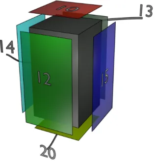
operations such as averaging, integration and differentiation. Instead of creating new groups we can import and adapt the geometric groups defined by the GEOM module. In Figure 3.10 we use the function import group from the SMESH module to perform this copy operation. The labels of the surfaces marked for boundary conditions and coupling interfaces are defined as follows. The inlet and the outlet of the reactor are labeled with 20 and 10 respectively. The reactor lateral surface are marked by 12,13, 14 and 15. The internal volume needed is label by 2. We recall that a number greater than 9 indicates a

(41)

Figure 3.11: Test 1. Coarse basic mesh for the three-dimensional reactor region. surface and less than 10 a volume by assumption. In Figure 3.11 the coarse basic mesh for the three-dimensional reactor region is shown. We recall that the coarse basic mesh must adapt over the assembly boundary. Mesh with elements that have surfaces between core assemblies is not allowed. A mesh refinement can be easily performed by using the FEMuS utility gencase in order to improve resolution inside the assembly grid.

3.2.3 Mono-dimensional primary loop mesh

Figure 3.12: Test 1. Sketch of the primary loop components.

(42)

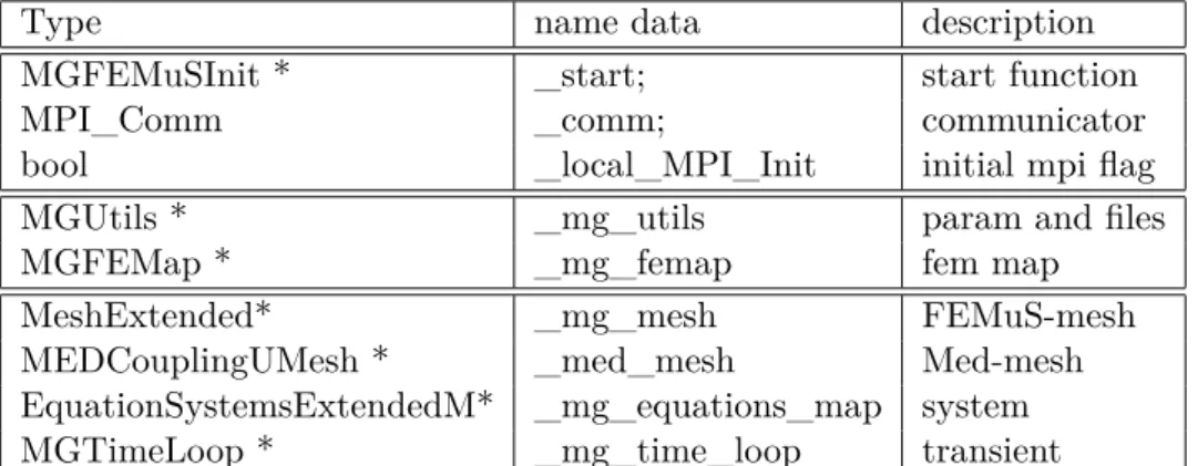
which is in this case the file circuit_test1.dat. The mesh can be generated by using GUITHARE, the graphical user interface on Salome platform. An overall sketch is shown in Figure 3.12. As said before in the mono-dimensional circuit the fluid exits from the point volume VOL enters the axial DOWNWARD, flows into the UPWARD branch and returns to the volume point VOL.

The mono-dimensional mesh is defined in the circuit_test1.dat produced by GUI-THARE. In Figures 3.13–3.16 details on the circuit components and its mesh are shown. The directive defining this circuit in the input deck are as follows

CIR = CIRCUIT UPWARD VOL3D DOWNWARD CIEL CALOPORT;

CIRCTOT = REACTOR CIR ;

There is only one circuit (labeled by CIR) which consists of 4 modules: UPWARD, VOL3D, DOWNWARD, CIEL. The UPWARD and DOWNWARD are axial mono-dimensional modules. VOL3D is a 0-mono-dimensional volume module and CIEL is a BCON-DIT module which is used to define pressure boundary condition in VOL3D. The key word CALOPORT is needed to identified the fluid. We define

CALOPORT = FLUID LEAD ;

at the beginning of the file to have lead as a coolant fluid. In Figure 3.13 Cathare

VOL-Figure 3.13: Test 1. The VOLUME module (VOL3D).

UME module (VOL3D) is shown. Here we report the corresponding Cathare command

lines for this VOLUME component

VOL3D = VOLUME JUPVOL USTREAM JVOLDOWN DSTREAM JCIEL DSTREAM ; GEOM VOL3D

(43)

Figure 3.14: Test 1. The BCONDIT CIEL module. 0.2 2.14

JUPVOL BOTTOM LENGTH 0. SECT .125 PERI .628 SIZE .2 VERTICAL JVOLDOWN BOTTOM LENGTH 0. SECT .125 PERI .628 SIZE .2 VERTICAL

JCIEL TOP LENGTH 0. SECT .125 PERI .628 SIZE .2 VERTICAL;

VOL3D is a VOLUME module (0-dimensional) with 3 junctions JUPVOL (USTREAM), JVOLDOWN (DSTREAM) and JCIEL (DSTREAM). The USTREAM and DSTREAM label indicates the circuit orientation. The geometry of VOL3D is defined by the key GEOM. We have two points at level z = 0.0 and z = 2.0m with constant section of 2.14m2_{. The other three lines define the geometry (length,section,perimeter,size) of} the junctions inside the VOLUME module. The junction direction is set vertical. The junction JCIEL is connect to the BCONDIT CIEL module. The BCONDIT CIEL module is described by

CIEL = BCONDIT JCIEL USTREAM ; MODEL CIEL BC5A

P REALLIST 1.01D5 1.01D5 1.01D5 1.01D5

ABSTIME REALLIST 0.0 0.1 100. 1.E+11 ;

The CIEL is a BCONDIT module with a junction JCIEL (USTREAM). The boundary condition model for CIEL is BC5A. The BC5A type of boundary conditions is an external outlet where one must specify only the pressure P. The pressure P is defined over three intervals of time [0, 0.1], [0.1, 100] and [100, 1.E+11]. In these three intervals the pressure is assumed to be constant at 1.01 × 105_{bar by the REALLIST command. In Figure 3.15} Cathare AXIAL DOWNWARD module is shown. The corresponding Cathare lines for this component are

(44)

Figure 3.15: Test 1. The AXIAL DOWNWARD module. DOW01 = XAXIS 0. ; DOW02 = XAXIS 7. ; DOW03 = XAXIS 9. ; DOW04 = XAXIS 9.4 ; LDOWARD = DOW01

SEGMENT 15 DOW02 COS -1. SEGMENT 20 DOW03 COS 0. SEGMENT 5 DOW04 COS 1. ; MESH DOWNWARD LDOWARD; GEOM DOWNWARD

(DOW01 AND DOW04) SECT 0.125 PERI 0.628 SIZE 0.2 ;

DOWNWARD is an AXIAL module with two junctions: JVOLDOWN (USTREAM) and JDOWNUP (DSTREAM). This component consists of 4 points: DOW01 (x = 0), DOW02 (x = 7), DOW03 (x = 9) and DOW04 (x = 9.4). It stars at the point DOW01 with 3 segments with 15 20 and 5 elements, respectively. The orientation of these three segment is defined by the cos directive: downward vertical for COS = −1, horizontal for COS = 0 and upward vertical for COS = 1. The section, perimeter and size of the pipe are define with the key directive GEOM. If the size is given the section and the perimeter can be automatically computed. In Figure 3.16 Cathare AXIAL UPWARD module is shown. Here we report the corresponding Cathare line for this component UPWARD = AXIAL JDOWNUP USTREAM JUPVOL DSTREAM;

UPW01 = XAXIS 9.4; UPW02 = XAXIS 16.0;

LUPWARD = UPW01 SEGMENT 15 UPW02 COS 1. ; MESH UPWARD LUPWARD;

(45)

Figure 3.16: Test 1. The AXIAL UPWARD module. GEOM UPWARD

(UPW01 AND UPW02) SECT 0.125 PERI 0.628 SIZE 0.2 ;

As written above the UPWARD component is an AXIAL connected between two junc-tions: JDOWNUP (USTREAM) and JUPVOL (DSTREAM). The USTREAM and DSTREAM label indicates the circuit orientation. The components has two points: UPW01 (x = 9.4) and UPW02 (x = 16). We remark that we have kept a unique coordi-nate system along the line for the UPWARD and DOWNWARD branch. There a unique segment with 15 element in the upward vertical (COS = 1) direction. The geometry is the same as the other AXIAL one.

The initial condition in the junction JDOWNUP is given as REALC JDOWNUP P 1.01D6 TL 400.0D0 HVSAT ALFA 1.0D-5 VL 1.0D-1 VV 1.0D-1; GOPERM;

The Cathare code is a two-phase code and even if we use only fluid coolant initial and boundary conditions for the other phase should be given. In this case we assume gas with the same temperature and velocity with gas fraction irrelevant (ALFA=1.0D-5). The computation direction is fixed by

(46)

We start from the UPWARD to VOL3D and to DOWNWARD. The CIEL BCONDIT is set at the end as usual.

3.2.4 Fuel distribution and pressure losses

The fuel and the pressure loss distribution are fundamental for the correct computation of the pressure and temperature fields. In this case we assume simple analytic distribution.

Figure 3.17: Distribution of the peak factor pk for fuel assembly.

In Figure 3.17 we show the distribution of the peak factor for fuel assembly for Test 1.

(47)

The peak factor pT is the ratio between the average source intensity and the assembly

value. The average volumetric source qav is set to

qav= 1.176156 × 108 (3.1)

The expression of the peak factor pL for pressure losses is set constant along the z

direction while over the plane is distributed as follows

pT(x, y) = 1.2 − .4 ∗ x ∗ (x − 3.66) ∗ y ∗ (y − 3.66) ∗ 16/167.9616 . (3.2)

The distribution is in parabolic form. In order to have maximum intensity on the edges of the reactor and the distribution bounded between 0.8 and 1.2 we subtract the parabolic distribution to the maximum peak value 1.2.

In a similar way in Figure 3.18 the distribution of the peak factor b for pressure losses are reported. The accidental pressure losses are assumed to be constant in a well specified vertical region. There is no particular physical sense for this assumption. The purpose of this choice is only to set enough intensity on a local region to that they can be seen in the the pressure solution when compared with gravity pressure losses.

3.2.5 Coupling FemLCore-Cathare on Salome platform for Test 1

The project should be written in the USER_APPL directory of the FEMuS code. This code has a directory structure similar to projects developed on Salome platform module and therefore we can reuse this structure again even for the Cathare input/output. The directory structure is shown in Figure 3.4. All the necessary files with the exception of the mesh file are contained inside the application directory FemLCore_cathare1. The input data files are in the DATA directory. The basic c++ files of the FemLCore code such as the Navier-Stokes and Energy equation solver together with Cathare links and FORTRAN files can be found in the SRC directory. The CFD three-dimensional mesh is in the MESH directory while the cathare.dat file defining the mono-dimensional geometry is stored in the SRC directory. The execuTable program is generated in this main directory while all the results both from FemLCore and Cathare are written in the

RESU directory. The coupling code starts three problems: P (FemLCore), C (Cathare)

and N problem (neutronics or heat sources).

The P problem is solved by the 3D-porous module of the FemLCore code. The P

prob-lem is defined by two parameter files: parameters.in and param_files.in. The MGUtils

class is the class that controls the parameter reading from the appropriate files stored in the DATA directory. Through the MGUtils class the parameters, the mesh and the basic structure directory name can be loaded. The coarse mesh is generated by the SALOME platform as discussed in Section 3.2.2. In this case we use a coarse mesh in MED Format contained in the file reactor.med The multigrid and multiprocessor mesh is generated by the gencase application by using the LIBMESH library [37, 38]. In order to assemble the discrete matrix of the Navier-Stokes and energy system with the Finite element method we need linear, quadratic and piecewise basis functions together with the topology of the appropriate geometric element. The appropriate MGFE and

(48)

Problem P Thermohydraulics Problem C Problem N Neutronics algebraic peaks Thermohydraulics 1D primary loop 3D core plena 3D Mesh Salome Med format FemLCore 3D Cathare 1D

Interface class Interface class Interface class

FemLCore 3D Cathare 1D CODE CODE Peaks algebric 1D mesh GUITHARE Cathare format SUPERVISOR main.cpp

Figure 3.19: Test 1. Schematic of the coupling computations

specify the equation system to be solved the std::vector<FIELDS> myproblemP must be filled. The dimension is 2 if Navier-Stokes system (NS_F) and energy equation (T_F) are to be solved. Once the utility classes (mgfemap(MGFE),mgutils[0](MGUtils), mgge-omel(MGGeomEl)) are initialized the P problem can be set by the following standard code lines

FEMUS P; // constructor

P.init_param(*mgutils[0]); // init parameter

P.init_fem(*mggeomel,*mgfemap);// init fem

// setting mesh

---P.setMesh(); // set MGmesh

// setting system ---P.setSystem(myproblemP,0,2); // set system 2 cell vector // setting inital condition at t=0

---P.solve_setup(itime_0,time); // initial time loop (t=0)

The FemLCore interface to Salome platform is called FEMuS. Each command needed to construct the problem is contained in this class. The parameters and the FEM element approximations are linked to the FEMuS interface and then to the FemLCore core class. The mesh in MED format is loaded in the FemLCore mesh structures. Two copies of the same mesh in different formats are allocated in the interface FEMuS class. This allows the transfer of data from the code to the Salome platform and viceversa. The function setSystem(myproblemP,0,2) initializes the system NS_F and T_F and allocates two piecewise-constant external fields. These external fields can be used by a neutronic code with the appropriate Salome interface. In order to exchange data from the three-dimensional simulation to the mono-three-dimensional one we need to define interface in the P Problem. The interfaces are created by writing

(49)

P.init_interface(33,10, 1,"mesh_file");// top pressure

P.init_interface(11,20, 2,"mesh_file");// bottom temperature P.init_interface(21,20, 2,"mesh_file");// bottom velocity P.init_interface(31,20, 1,"mesh_file");// bottom pressure

From Figure 3.20 we can see the location of the groups defined from mesh generator. With the first line the group 10 is associated with top surface which is the outlet of the reactor. However on the top surface we need to transfer data for the temperature and pressure fields. Therefore the interface with name 10 is created on the mesh group 10 for quadratic temperature field and the interface with name 33 is created on the mesh group 10 for linear pressure field. It is important to remark that the creation of the interface generates a local mesh which is quadratic and all the linear functions must be adapted over a coarser mesh. The bottom surface is the inlet of the reactor where we need to exchange temperature, velocity and pressure. For this reason three interfaces labeled 11, 21, 31 are defined over the same mesh geometric group 20.

The generation of the heat source is called N Problem. Since we are not interested in neutronic computations, the interface with a neutronic code is substituted by a simple interface that generates a semi-analytic heat source profile. This simple interface is defined by the ReactData class. In order to define the N Problem we write

ReactData *N;

N = new ReactData();

N->datagen(P.get_MGExtSystem());

N is therefore the interface that controls the data flow for the heat and pressure loss

sources inside and out of the reactor.

(50)

The C problem is a Cathare problem. The interface class is called Problem_Cathare. The initialization of this class can be done simply by

Problem_Cathare* c = new Problem_Cathare(); c->initialize();

The interface points for the Cathare problem can be defined as in Table 3.1. At the the

location name component position (ix) rad (irad)

inlet point 1 DOWNWARD 40 0

outlet point 2 DOWNWARD 1 0

pump pump pt DOWNWARD 25 0

exchanger heat_ex pt DOWNWARD 25 0

Table 3.1: Test 1. Cathare key interface points.

point 1 located at the inlet, with coordinates x = ix_1 of the DOWNWARD module we can get all the variables with the following Cathare interface command

rho_1=c->getValue_Cathare("LIQDENS","DOWNWARD",ix_1,0); f_1=c->getValue_Cathare("LIQFLOW","DOWNWARD",ix_1,0); P_1=c->getValue_Cathare("PRESSURE","DOWNWARD",ix_1,0); h_1=c->getValue_Cathare("LIQH","DOWNWARD",ix_1,0); T_1=c->getValue_Cathare("LIQTEMP","DOWNWARD",ix_1,0); v_1=c->getValue_Cathare("LIQV","DOWNWARD",ix_1,0);

With LIQDENS, LIQFLOW, PRESSURE, LIQH, LIQTEMP and LIQV as arguments this function returns the value of density, mass flow, pressure, enthalpy, temperature and velocity, respectively.

The pump and the heat exchanger are set in the DOWNWARD module. The pump model, which is located at the coordinate x = ix_p, is very simple. In the pump point we impose a constant pressure with

c->setValue_Cathare("DPLEXT","DOWNWARD",ix_p,0,DP);

where ix_p and irad are defined as in Table 3.1. DP= .75 × 105_{Pa is the pump gain} in pressure. The heat exchanger is located on the DOWNWARD module at the point with coordinates x = ix_h, see Table 3.1. The heat exchanger can be modeled by the following code lines

T_ex=c->getValue_Cathare("LIQTEMP","DOWNWARD",ix_h, 0); h_ex=c->getValue_Cathare("LIQH","DOWNWARD",ix_h, 0); h_ex1 = h_ex -w_ex*(cp*(T_ex-T_ex2));

c->setValue_Cathare("ENTLEXT","DOWNWARD",ix_h,0,h_ex1);

The cooling temperature Tex2is set to 400C. The enthalpy hex is determined iteratively

to the corresponding value of the cooling temperature Tex2. The constant wex is the

(51)

At the point 1 and point 2 defined in Table 3.1 we have the 3D/1D interfaces. At the point 2 the three-dimensional state must pass the temperature value to the Cathare code. The mono-coordinate of the Cathare code of the point 2 is labeled ix2. In order to set the temperature we use a feedback algorithm. Let Toutrbe the average temperature that

flows out from the three-dimensional reactor and t21/h21 be the temperature/enthalpy on the other side of the interface on the Cathare mono-dimensional mesh (point 2). The temperature t21 is corrected until it reaches Toutr by these code lines

t_21=c->getValue_Cathare("LIQTEMP","DOWNWARD",ix_2,0; h_21=c->getValue_Cathare("LIQH","DOWNWARD",ix_2, 0; h_12 = h_21-(cp*(t_21-T_outr)); // hentalpy correction c->setValue_Cathare("ENTLEXT","DOWNWARD",ix_2, 0,h_12);

The pressure coupling is obtained by imposing the three-dimensional average pressure drop P [0] − P0[0] to the mono-dimensional part of the circuit between the point 1 and point 2. In this way we correct the mono-dimensional drop with the correct one. We write the following code lines

press_p2=c->getValue_Cathare("PRESSURE","DOWNWARD",ix_2,0); press_p1=c->getValue_Cathare("PRESSURE","UPWARD",ix_1,0); dp_ioo=c->getValue_Cathare("DPLEXT","UPWARD",2,0); dp_io=dp_ioo-0.5*(fem_rho*(h*g+averageP[0]-averageP0[0])-(press_p1-press_p2)); dp_io=dp_ioo; c->setValue_Cathare("DPLEXT","UPWARD",2,0,dp_io);

On the inlet section of the reactor we need to set temperature and velocity field. Since we do not know the field distribution at the reactor we assume a constant distribution. The temperature T1 from the point 1 of Cathare should be imposed to the inlet reactor. We write

// Temperature coupling T_1(Cathare) with interface 11(bottom) std::ostringstream a; a<< T_1;

P.setAnalyticBoundaryValues(11,1, a.str().c_str());

P.write_Boundary_value(11,"T",1);// write inside x_old sol and for the velocity field we write

// velocity coupling v_1(Cathare) with interface 21 (bottom) std::ostringstream vel; vel<< "IVec*0.+JVec*0+KVec*"<< v_1; P.setAnalyticBoundaryValues(21,3, vel.str().c_str());

P.write_Boundary_value(21,"NS0",3); // write inside x_old

The boundary conditions for temperature and velocity are imposed directly by using the FEMuS interface functions write_Boundary_value directly on the old solution vector