Phenomenological analysis of near-threshold periodic modulations of the proton timelike form factor

Phenomenological analysis of near threshold periodic modulations

of the proton time-like form factor

A. Bianconi∗

Dipartimento di Ingegneria dell’Informazione, Universit`a di Brescia and Istituto Nazionale di Fisica Nucleare,

Gruppo Collegato di Brescia, 25133 Brescia, Italy

E. Tomasi-Gustafsson†

Abstract

We have recently highlighted the presence of a periodically oscillating 10 % modulation in the BABAR data on the proton time-like form factors, expressing the deviations from the point-like behavior of the proton-antiproton electromagnetic current in the reaction e++ e−→ ¯p+p. Here we deepen our previous data analysis, and confirm that in the case of several standard parametrizations it is possible to write the form factor in the form F0+ Fosc, where F0is a parametrization expressing the long-range trend of the form factor (for q2 ranging from the ¯pp threshold to 36 GeV2), and

Fosc is a function of the form exp(−Bp) cos(Cp), where p is the relative momentum of the final ¯

pp pair. Error bars allow for a clean identification of the main features of this modulation for q2 < 10 GeV2. Assuming this oscillatory modulation to be an effect of final state interactions between the forming proton and the antiproton, we propose a phenomenological model based on a double-layer imaginary optical potential. This potential is flux-absorbing when the distance between the proton and antiproton centers of mass is >_{∼ 1.7-1.8 fm and flux-generating when it is}

<

∼ 1.7-1.8 fm. The main features of the oscillations may be reproduced with some freedom in the

potential parameters, but the transition between the two layers must be sudden (0-0.2 fm) to get the correct oscillation period. The flux-absorbing part of the ¯pp interaction is well known in the

phenomenology of small-energy antiproton interactions, and is due to the annihilation of ¯pp pairs

into multi-meson states. We interpret the flux-creating part of the potential as due to the creation of a 1/q-ranged state when the virtual photon decays into a set of current quarks and antiquarks. This short-lived compact state may be expressed as a sum of several hadronic states including the ones with large mass Qn ≫ q, that may exist for a time t ∼ 1/(Qn− q). The decay of these large mass states leads to an intermediate stage regeneration of the ¯pp channel.

PACS numbers: 12.40.Nn Regge theory, duality, absorptive/optical models 13.40.Gp Electromagnetic form factors

∗_{E-mail: andrea.bianconi@unibs.it} †_{E-mail: etomasi@cea.fr}

I. INTRODUCTION

Both the annihilation reactions

e++ e− → ¯p + p, (1)

¯

p + p→ e++ e−, (2)

have been used to extract the electromagnetic form factors (FFs) of the proton in the time-like (TL) region (for a recent review see [1] and references therein). Assuming that the interaction occurs through one photon exchange, the annihilation cross section is expressed in terms of the FF moduli squared, as FFs are of complex nature in the explored kinematical region [2].

The collected statistics has not permitted the individual determination of the electric (GE) and magnetic (GM) FFs due to the available limited luminosity. The cross section σ of the reactions (1) and (2), allows to extract the squared modulus of an effective form factor Fp, that is in practice equivalent to the assumption GE = GM (strictly valid only at threshold) [3]: |Fp|2 = 3βq2_σ 2πα2 ( 2 + 1 τ ), (3)

where α = e2_{/(4π), β =} √_{1− 1/τ, τ = q}2_/(4M2_{), q}2 _{is the squared invariant mass of the} colliding pair, and M is the proton mass. The effect of the Coulomb singularity of the cross section at the ¯pp threshold is removed by the β factor: β → 0 for q → 2M, so that βσ is finite and the effective form factor is expected to be finite at the threshold.

The reactions (1) and (2) test close-distance components of the wave function of the ¯pp system, that are supposed to be suppressed because of ¯pp annihilation. Data on the ¯p-nucleon and ¯p−nucleus annihilation process at low energies (see [4–16], and the related theoretical analyses [17–19]) show that a proton and an antinucleon overlap little. When their surfaces come in touch, or even within a distance of 1 fm, they annihilate into other hadron states. Elastic scattering is present, but either of diffractive origin (for p≫ 100 MeV), or of refrac-tive repulsive hard-core nature (near threshold). In all cases, the wave function of the ¯pp relative motion is estimated to be strongly suppressed at distances lower than 1 fm. On the other side, reactions (1) and (2) involve a virtual photon with center of mass (c.m.) energy √

formed (or decays) have size ∆r ≤ 0.1 fm. So, the virtual photon tests the short-distance components of the ¯pp system, and TL FF complement, in this respect, the information acquired from other annihilation experiments.

Until recently, uncertainties and discontinuities between data coming from different mea-surements have prevented from appreciating the continuity features of TL FF data over a large q2 _{range. The recent results from the BABAR collaboration [20, 21], cover a q}2 _range going from near the threshold to 36 GeV2, with more than 30 data points only in the region q2 _{< 10 GeV}2_.

Specific features of the effective FF related to final state interactions between ¯p and p appear when expressing |Fp(q2)|2 in terms of the 3-momentum of the relative motion of the two hadrons. This has been illustrated in a recent work [22], where we have highlighted periodic features in a modulation of the order of 10 % , superimposed on the long-range trend of the effective FF. The precision of the available data does not forbid the interpretation where the oscillation pattern is attributed to independent resonant structures, as in Ref. [23]. However, the underlying assumption of the present work is that the oscillations are expression of a unique interference mechanism, affecting all the q2 _{range where the oscillations are} visible. Of course, the two points of view may coexist within a model where two or more resonance poles are the result of a global underlying mechanism, as in [24], or within a duality framework. As observed in our final discussion, the proposed phenomenological interpretation may be framed within several models, including multiple-pole ones.

In the present work we first scrutinize these oscillations by expanding the data analysis of Ref. [22]. We use four different parametrizations from the literature for the so-called ”background” term (the effective form factor as it appears if one neglects the small oscillating modulation). For each choice of the background, we fit the residual modulation, visible in the difference between the data and the background fit. We analyze the uncertainty on the periodical character of the oscillations, and on their possible long-range scaling behavior (Section II).

Next, we present a phenomenological model for the rescattering origin of the oscillations, within a DWIA (distorted wave impulse approximation) scheme where the outgoing (or incoming) hadron waves are distorted by an optical potential (Section III). In absence of distorting potentials, the background form of the TL FF is recovered (Section IV). This analysis shows that it is possible to reproduce most of the features of the observed oscillations

this way, but important constraints must be satisfied by the rescattering potential (Section V). Conclusions summarize the main finding of the paper.

II. ANALYSIS OF THE DATA

The effective proton FF extracted from BABAR data on e+_{+ e}− → ¯p + p(γ) [20, 21], is reported in Fig. 1 (black circles) as a function of q2_{, that is equivalent to the total energy} squared s in the TL region. As it can be noticed in the insert that highlights the near threshold region, 4M2 _{≤ q}2 _{≤ 10 GeV}2_{, the data show irregularities. These irregularities} acquire a peculiar structure when q2 is replaced by the relative momentum of the ¯pp system in the rest frame of one of the hadrons [22].

We introduce a function of the form

F (p) ≡ F0(p) + Fosc(p) (4)

where

1. The 3-momentum

p(q2) ≡ √E2− M2_{, E} ≡ q2_{/(2M )} − M. ₍₅₎ is the momentum of one of the two hadrons in the frame where the other one is at rest.

2. F0(p) (”regular background term” ) is a function expressing the regular behavior of the FF over a long q2 _range.

3. Fosc(p) describes the deviation of the TL FF from the long-range regular background appearing in the region 0 ≤ p <_{∼ 3 GeV and corresponding to M ≤ q ∼ 3 GeV,}< with q =√q2_.

Different forms available from the literature can be used for the background term. As measured by BABAR, F0[p(q)] is slightly steeper than expected on the ground of the corre-sponding fits of the space-like (SL) FF (dipole-like shape) and of the power law correcorre-sponding to quark-counting rules [25, 26]. The recent data are best reproduced by the function FR

proposed in [27] that we will use as a reference: |FR|(q2)| = A (1 + q2_/m2 a) [1− q2/0.71] 2, A = 7.7 GeV−4_{, m}2 a = 14.8 GeV 2 . (6)

Other parametrizations have been proposed. The world data prior to BABAR results were well reproduced in the experimental papers [28] according to the function:

|FS(q2)| = A

(q2₎2_log2_(q2_/Λ2₎, (7)

where q2 _{is expressed in GeV}2_, A = 40 GeV−4 _{and Λ = 0.45 GeV}2_.

The functional form of Eq. (7) is driven by the extension to the TL region of the dipole behavior. The dipole model of the SL FFs, more precisely their (q2)2 dependence, is em-pirically well known since the first elastic scattering experiments [29] and agrees with most of the nucleon models developed during last century, as for example, the constituent quark model of Ref. [30]. It is also consistent with PQCD large-q2 _{predictions [26].}

Based on Ref. [31], in order to avoid ghost poles in αs, the following modification was suggested ([32]) :

|FSC(q2)| =

A (q2₎2[_log2

(q2_/Λ2_{) + π}2]. (8)

In this case the best fit parameters are A = 72 GeV−4 and Λ = 0.52 GeV2_.

In Ref. [24] a form was suggested with two poles of dynamical origin (induced by a dressed electromagnetic current)

|FT P(q2)| =

A (1− q2_/m2

1)(2− q2/m22)

. (9)

The best fit parameters are A = 1.56, m2

1 = 1.5 GeV2 and m22 = 0.77 GeV2. The parametrizations with the best fit parameters are illustrated in Fig. 1 and summarized in Table I. The best fit functions are then subtracted from the data, leaving a regular oscillatory behavior, Fig. 2. It has magnitude ∼ 10 % of the regular term, and is well visible over the data uncertainties for p > 3 GeV. We have fitted the difference between the BABAR data and the regular background term F0(p) with the 4-parameter function

Fosc(p) ≡ A exp(−Bp) cos(Cp + D). (10)

Let us focus on the case F0 = FR, Eq. (6). The corresponding difference data are plotted in the lower panel of Fig. 2a. The relative errors in the parameters C and B show that the

]

[GeV

q

10

20

30

40

F

10

10

10

FIG. 1: (color online) Data on the TL proton generalized FF as a function of q2, from Ref. [20, 21] together with the fits from Eq. (6) (black solid line), Eq. (7) (blue dash-dotted line), Eq. (8) (red dashed line), and Eq. (9) (Green, long-dashed line). The insert magnifies the near threshold region. Because of their large error bars, the points over 16 GeV2 do not affect fit parameters, so that the four fits best reproduce the data in the insert, apart for the oscillations that are the focus of this work.

oscillation period is better defined than the damping coefficient exp(−Bp). Two and a half oscillations are clearly visible over the reaction threshold, while for p > 2.8 GeV the vertical error bars overcome the oscillation amplitude A exp(−Bp).

The parameter D defines the position of the first oscillation maximum that occurs at p = 0 within the error ∆D P/(2π), where P is the oscillation period. Estimating the oscillation period P = 1.13 GeV, the first oscillation maximum occurs at p = 0 within an error of 0.05 GeV. Five peaks (maxima and minima) are visible and the periodicity hypothesis, that is implicit in the cos(Cp + D) term implies that they are regularly spaced by a half-period of 1.13/2 GeV. Examining Fig. 2a (lower panel) we find:

0 1 2 3 p F 0.1 0.2 0.3 (a) p [GeV] 0 1 2 3 D 0.04 − 0.02 − 0 0.02 0.04 (b) 0 1 2 3 p F 0.1 0.2 0.3 p [GeV] 0 1 2 3 D 0.04 − 0.02 − 0 0.02 0.04 0 1 2 3 p F 0.1 0.2 0.3 p [GeV] 0 1 2 3 D 0.04 − 0.02 − 0 0.02 0.04 0 1 2 3 p F 0.1 0.2 0.3 p [GeV] 0 1 2 3 D 0.05 − 0 0.05 (d) (a) (c) (b) Fp p [GeV] D D D Fp Fp D Fp p [GeV]

FIG. 2: Referring to Eqs. (4) and (5), we report the background fits F0(p) of the BABAR data, according to the four parametrizations a) F0 = FR from [27] (Eq. (6), see text or Table 1), b)

F0 = FS from [28] (Eq. (7)), c) F0 = FSC from [31] (Eq. (8)), d) F0 = FT P from [24] (Eq. (9)), and the corresponding fits Fosc(p) of the differences between the data and each parametrization. In all the four cases Foschas the damped oscillation form of Eq. (10), with the best-fit parameters reported in Table 1. For each insert: (top) the data of BABAR are plotted, together with the parametrization F0(p) (blue, dashed line) and the complete fit FR(p) = F0(p) + Fosc(p) (solid black line); (bottom) the difference of the data and the parametrization is shown, together with the fit

Fosc(p) (solid red line).

• 1st minimum: estimated at 0.57 GeV, visible inside the range 0.5-0.6 GeV, • 2nd maximum: estimated at 1.13 visible at 1.1 GeV with negligible uncertainty, • 2nd minimum: estimated at 1.7 GeV, visible inside the range 1.7-1.8 GeV, • 3rd maximum: estimated at 2.26 GeV, visible inside the range 2.2-2.3 GeV,

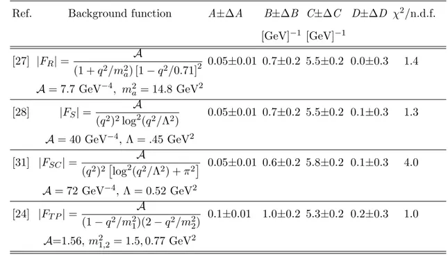
TABLE I: Background fit functions from Eqs. (6, 7, 8, 9) (see Fig. Fig:WorldData), and parameters

A, B, C, D (with the related χ2/n.d.f.) for Eq. (10 ) fitting in each case the difference between the data and the corresponding background function.

Ref. Background function A±∆A B±∆B C±∆C D±∆D χ2/n.d.f. [GeV]−1 [GeV]−1 [27] |FR| = A (1 + q2_/m2 a) [1− q2/0.71] 2 0.05±0.01 0.7±0.2 5.5±0.2 0.0±0.3 1.4 A = 7.7 GeV−4, m2_a= 14.8 GeV2 [28] |FS| = A (q2₎2_log2_(q2_/Λ2₎ 0.05±0.01 0.7±0.2 5.5±0.2 0.1±0.3 1.3 A = 40 GeV−4_{, Λ = .45 GeV}2 [31] |FSC| = A (q2₎2[_log2_(q2_/Λ2_{) + π}2] 0.05±0.01 0.6±0.2 5.8±0.2 0.1±0.3 4.0 A = 72 GeV−4_{, Λ = 0.52 GeV}2 [24] |FT P| = A (1− q2_/m2 1)(2− q2/m22) 0.1±0.01 1.0±0.2 5.3±0.2 0.2±0.3 1.0 A=1.56, m2 1,2= 1.5, 0.77 GeV2

• 3rd minimum: estimated at 2.83 GeV, visible inside the range 2.6-2.9 GeV.

The largest uncertainty in the position of the peak is found in the last case. Excluding this one, in the other cases the relative discrepancy lies within (0.1 GeV / 0.57 GeV) ≈ 15 %. This justifies the presence of the periodic term cos(Cp + D) in the fit. Such analysis may be repeated for the other cases in Fig. 2, with similar results.

Concerning the amplitudes of the half-oscillations, each of them is about 1/√2 of the previous one, so that each maximum of Fosc(p) is about 1/2 of the previous maximum. This motivates the use of exp(−Bp) in the fit, although in this case the error on this “1/√2 rule” is too large to exclude good fits with other analytic shapes. In particular, one possibility is that the oscillation amplitude is proportional to the background term, so that the overall fit would assume the form F0(p)[1 + ϵ cos(Cp)] with constant ϵ ≈ 0.1. For increasing momenta within the visible range, the damping of the oscillation and of the regular background term are similar: Fosc(p)/F (p)≈ constant, both decreasing by 1/e in about 1.4-1.5 GeV.

Since increasing relative errors hide the possible presence of the oscillations for p > 3 GeV, we cannot know whether the oscillations are relevant at larger p or not. Assuming that they are, the point of view supported in our previous work [22] and in the following is

that we are facing an interference effect between a small number of amplitudes, effectively competing in the visible momentum range. These amplitudes must be few, not forming a regular continuum, otherwise they would give rise to a diffraction pattern, rather than an oscillation pattern. comment that Note that the oscillatory behavior is present already in the cross section, and in other invariant functions of q2_{, but not periodic. A relevant point} is that Fosc(p) is periodic with respect to p, not with respect to q2 or q. Since p is a variable that is uniquely associated with the relative motion of the hadron, we associate periodicity with interactions between the forming hadrons after the virtual photon has been converted into quarks and antiquarks, Eq. ( 1), or before quarks and antiquarks annihilate into a virtual photon, Eq. (2). In both cases we name ”rescattering” these interactions.

III. OPTICAL MODEL

We assume that rescattering is a relatively small perturbation, and that in absence of rescattering the effective FF would coincide exactly with F0(p). We also assume that it is possible to neglect the dependence of the rescattering mechanism on q2_.

Let ⃗r be the space variable that is Fourier-conjugated to ⃗p: r is the distance between the centers of mass of the two forming hadrons, in the frame where one is at rest. The observed behavior is modeled via a two-stage process where:

• In the e+_e− _{→ ¯pp ”bare” process a ¯pp pair is formed at a distance r with space} distribution amplitude M0(r).

• Rescattering takes place between the newly formed hadrons (p and ¯p) according to an optical potential that is function of their distance r.

To introduce rescattering we use the Distorted Wave Impulse Approximation (DWIA) formalism, following the scheme employed in Ref. [33]. The starting point is the Fourier transform

F0(p) ≡ ∫

d3⃗r exp(i⃗p· ⃗r)M0(r) (11)

where we interpret exp(i⃗p· ⃗r) as the plane wave final state of the ¯pp pair in their center of mass, and M0(r) as a matrix element describing the earlier stage of the process. Neglecting

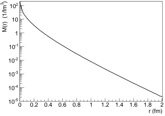
r (fm) 0 0.2 0.4 0.6 0.8 1 1.2 1.4 1.6 1.8 2 ) 3 M(r) (1/fm -5 10 -4 10 -3 10 -2 10 -1 10 1 10 2 10 M(r)

FIG. 3: The 3-dim Fourier transform M0(r) of F0(p), defined in Eq. (11).

rescattering, a detailed model for the formation process would lead to a matrix element of the form

F0(p) = < ψf(x1, ..., xn)ψf(⃗r)|T (r, x1, .., xn, xe+_e−)|ψ_i(x_e+_e−) >

≡ ∫

d3⃗r ψf(⃗r) M0(r), (12)

where the hard operator T is sandwiched between the initial state ψi, that is function of the 4-vector x_e+_e− expressing the relative coordinates of the e+e− pair, and the final states

ψf that depend on the internal coordinates x1, x2, ...xn of the two hadrons as well as on their relative position ⃗r. The result of integrating over all variables but r, is M0(q2, r), that in general depends on q2 since this is a parameter of ψi and ψf. We assume that this dependence may be neglected in the range 0 < p < 3 GeV where the oscillations are distinguishable from the background.

Plane Wave Impulse Approximation (PWIA) corresponds to the absence of rescattering:

ψf(⃗r) = exp(i⃗p· ⃗r) . (13)

of ¯pp rescattering. We choose a simple factorized distortion D(⃗r)

ψf(⃗r) = D(⃗r) exp(i⃗p· ⃗r) , (14) where D(⃗r) is calculated as a Glauber-like eikonal factor:

D(x, y, z) = exp ( − ib ∫ _∞ z ρ(x, y, z′)dz′ ) (15)

where ˆz // ⃗p and b is a complex number, whose meaning is:

• Pure real b: elastic rescattering potential, that may be attractive or repulsive depend-ing on the relative sign of Re(b) and pz.

• Pure imaginary b: imaginary potential causing flux absorption or flux creation in rescattering.

Strictly speaking the product bρ(⃗r) is not a potential. V (r) ≡ 2bpρ(⃗r) is a true optical potential appearing in a linearized form of the Schrodinger equation, but for simplicity we name ”potential” the product bρ(⃗r).

The key function is the real function ρ(r), describing the space distribution of the strength and the sign of the rescattering potential (ρ may be negative). We have tested three families of space densities ρ(r) for the rescattering potential:

1. Compact rescattering densities: they are decreasing functions of r, as for example Woods-Saxon densities. This class includes imaginary-dominated potentials that are typical of the theory of ¯pp low-energy interactions.

2. Hollow rescattering densities: they are very small or vanishing at small r, large in a sub-range of 0.2-2 fm, and tend to zero for larger r.

3. Double-layer rescattering densities: these are the combination of two potentials of class 2 with opposite sign. So we may have a region ra < r < rb with a repulsive potential and a region rc < r < rd with an attractive potential, or we may have two regions, characterized by an absorbing and a generating imaginary potential.

All the potentials considered here act in a range that is typical of strong interactions. Elec-trostatic potentials have not been considered, since the short-range scheme used here is not suitable for analyzing phase shifts that develop at distances≫ 1 fm.

Summarizing, we calculate F (p) as F (p) = 1 (2π)3 ∫ d3⃗r ei⃗p·⃗rD(⃗r)M0(r), (16) M0(r) ≡ ∫ d3⃗p e−i⃗p·⃗rF0(p), (17)

with D(⃗r) defined in Eq. (15). We observe that F (p) does not depend on the orientation of ⃗p because of the choice of constraining the z-axis to the direction ⃗p in the calculation of D(⃗r).

IV. MODEL RESULTS

After testing several configurations, the results are the following.

1) Compact potentials.

Spherical homogeneous potentials (constant up to a fixed radius), Gaussian potentials and Woods-Saxon potentials do not give positive results. Neither real nor imaginary potentials have produced periodic oscillation patterns. This is in contrast with the case of the angular distributions of nuclear physics (see for example [33] where evident periodic patterns are obtained via pure imaginary Woods-Saxon densities). However, in those applications the relevant variable is the t−channel momentum exchanged in elastic scattering or rescattering, while here it is the relative momentum of the colliding particles, that is equivalent to an s−channel momentum.

2) Hollow potentials (not changing sign or phase in the r range of interest).

We have tested simple double-step potentials (constant between two r values, zero else-where), and shifted-Gaussian potentials exp[−(r − r0)2/σ2], with both real and imaginary parts. Real hollow potentials produce periodical oscillations, but the oscillation period is far too large (2 GeV or more). In order to make it shorter, the peak value of the potential has to be pushed to r > 2 fm. M0(r) decreases by 3-4 orders of magnitude when r increases by 1 fm (see Fig. 3). So, at distances > 2 fm M (r) is very small, depriving of relevance the effects of a real potential that is active in these regions. Imaginary potentials of pure absorbing (or pure generating) class have been found to be incompatible with our starting requirement that rescattering is a small correction. For a hollow imaginary potential to produce oscillations with relative magnitude 10 %, one needs a strong imaginary potential, which leading effect is damping by orders of magnitude the unperturbed term.

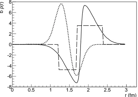
r (fm) 0 0.5 1 1.5 2 2.5 3 (r) ρ b -8 -6 -4 -2 0 2 4 6 8

Potential functions

FIG. 4: The three double-layer potentials used for the fits reported in figures 5, 6, and 7. Dashed curve: potential n.1 (Eq. (18)). Continuous curve: potential n.2 (Eq. (19)). Dotted curve: potential n.3 (Eq. (20)). These potentials are used in Eq. (15) to calculate the final state distortion factor D(x, y, z), that leads to the fit F (p) through Eq. (16).

3) Double layer potentials (presenting two r-ranges where the potential phase is

op-posite). Double-layer real potentials produce weaker oscillation effects than single-layer (hollow) potentials. Our best results have been obtained with double-layer imaginary po-tentials. These have been able to produce periodic oscillations with a period of 1 GeV or shorter, and of arbitrarily large amplitudes, depending on the parameters. Such potentials present an inner region where the ¯pp flux is produced and an outer region where the ¯pp flux is absorbed. The physical origin of this class of potentials is discussed in next section.

We report the results corresponding to the three different double-layer potentials illus-trated in Fig. 4. All of them are purely imaginary (Re(b)≡ 0). The former two potentials have been calibrated to reproduce, as well as possible, BABAR data. The third one presents peculiar features and non-optimal parameters, and it is reported for comparison discussion.

Potential n.1: Multiple-step function

Im(b)ρ(r) =: 0 for r < 1 fm and r > 2.4 fm; −4.8 for (1.2 < r < 1.7) fm;

3.5 for (1.7 < r < 2.4) fm; (18)

Potential n.2: Potential similar to the previous one, but regular:

Im(b)ρ(r) = B G(r− r0)T (r− r0)W (r− r0), (19) where

• B = 7.8 is an overall strength coefficient.

• G(r − r0) = exp[−(r − r0)2_/0.52_{] is a Gaussian with center in r}

0 = 1.8 fm, and width µ = 0.5 fm.

• T (r − r0) = tanh[(r− r0)/0.05] is a ”soft sign function”, that is equal to−1 for r ≪ r0 fm, to +1 for r ≫ r0 fm, and changes smoothly sign in a range of 0.1 fm.

• W (r − r0) = 1 + 0.05(r− r0) is a weight function that (slightly) increases the strength of the external absorbing peak over the internal generating one.

Potential n.3: Sum of a positive Gaussian in the inner region and a negative one in the

outer region:

Im(b)ρ(r) = A+G+(r− r+)− A−G−(r− r−), (20) with G± ≡ exp(−[(r − r±)2/w2], r+ = 1.35 fm, r− = r++ w, and w = 0.26 fm, A+=10, A−= 8.4.

This potential is very different from the previous two: the sign of the inner and outer parts are reversed (absorption inside), the average radius is smaller, the negative and positive peaks are more distant. It is reported here to highlight some effects of the parameters rather than for good fit purposes.

The results obtained with these potentials are presented in Figs. 5, 6, and 7. The fits with potentials 1 and 2 reproduce satisfactorily well the data, given the simplicity of the model. In these two cases, the data are slightly overestimated near the threshold. This may be attributed to the small-energy limitations of the eikonal formalism chosen here to

reproduce the wave distortion. As observed in [33] the use of this approximation within DWIA is good when several partial waves are involved in rescattering, and definitely it does not apply in a regime of S-wave dominance, corresponding to p≤ 200 MeV for ¯pp systems [17].

The example with potential n.3 shows that it is possible to obtain similar qualitative results with opposite configurations: absorbing potential in the outer region and generating potential in the inner region, or viceversa. For our best fits we have preferred the first option, because it corresponds to the phenomenology of ¯pp annihilation, dominated by flux absorption when the proton and antiproton begin to overlap.

Potential n.3 allows for an easy analysis of the separate role of the two potential layers, since one may independently modify the peak strengths A+ _{and A}−_{. Systematic attempts} show that it is possible to obtain periodic oscillations of pretty large amplitude by increasing both A+ _{and A}−_{, at the condition that the relative effect of the absorbing and of the} creating parts of the potential is well balanced, that may be obtained by acting on the ratio A+/A−. Apart for avoiding normalization problems, an equilibrated balance between the two strengths is one of the keys to get remarkable and periodic oscillations.

On the other side, this potential is not suitable for producing arbitrarily short oscillation periods, because it lacks a decisive feature of potentials n.1 and 2: their steep derivative at the point where they change sign. To obtain this feature with potential n.3, the distance between the two peaks must be smaller than their width. In such conditions the two Gaus-sians overlap and cancel reciprocally. We have been able to reduce the oscillation period down to what is visible in Fig. 7, but not further. The conclusion is that the period of the oscillations is related to a sudden transition between the flux feeding and the flux depleting regions.

Another important property shared by the three double-layer potentials is to produce a systematic threshold enhancement: p = 0 corresponds to an oscillation maximum, if the effect of the flux-creating and flux-absorbing parts of the potential are reasonably well balanced. This property is very stable, it is not related to a special set of parameters, and does not depend on the fact that the absorbing part of the potential is external (potentials n.1 and n.2) or internal (potential n.3). So, the threshold enhancement is an intrinsic property of the imaginary double-layer model.

used to fit ¯pp LEAR data [7, 17–19]. To reproduce LEAR elastic and annihilation data, phenomena taking place at small r have no relevance, since the surface interaction at r ≈ 1-2 fm prevents most of the initial ¯pp channel wave function from entering the r < 1 fm region. The ”regeneration” effect due to the inner potential introduced above would have little effect on the total elastic and inelastic cross sections, since it affects only a very small component of the wave function.

On the other side, this small component which is nonzero at small r is essential for the coupling of the proton-antiproton pair with a virtual photon with virtuality q2 _{> 4M}2_{. The} coupled regeneration/absorption mechanism introduced here produces, for r < 2 fm, an al-ternance of regions where this component of the ¯pp wave function is enhanced or suppressed. Let us discuss the conditions leading to observable effects. The enhancement of the cross sections at small p, where the the ¯pp distorted wave function exp[i⃗p· ⃗r]D(⃗r) approximately reduces to D(⃗r) and the Fourier transform of Eq. (16) simplifies to∫ d3_rD(⃗r)M

0(r), suggests that the potential enhances the wave function at small r where M0(r) is very large (see Fig. 3). This effect is not specific of double-layer potentials: for example with a spherical real attracting potential does the same. The presence of further oscillations at larger p however suggests that double-layer imaginary potentials create regions where the product D(⃗r)M0(r) alternatively becomes larger and smaller, enough to ”resonate” with the Fourier transform factor exp(i⃗p· ⃗r) for periodic p values far from the threshold (see Fig. 3b of [22]). If two regions with a larger and a smaller value of D(⃗r) are present at r+ and r− respectively, r+− r− must be small, or the steep r-decrease of M0(r) will make the modulation by D(r+) negligible with respect to D(r₋). This may explain the relevance of having a steep potential at the change of sign.

V. HYPOTHESIS ON THE PHYSICAL ORIGIN OF ”INNER CREATIVE/

OUTER ABSORPTIVE” POTENTIALS

An optical potential with an imaginary part may be justified within several theoretical frameworks but in general, and intuitively, its origin is related to the fact that a a multi-channel process is inclusively projected onto one multi-channel alone.

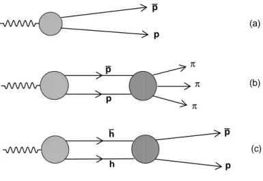
For the case of interest, this is illustrated in Fig. 8. Diagram (a) is the amplitude of γ∗ → ¯pp within a model that does not include ¯pp rescattering. This is supposed to lead

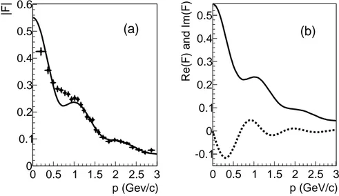
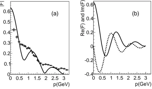
p (Gev/c) 0 0.5 1 1.5 2 2.5 3 |F| 0 0.1 0.2 0.3 0.4 0.5 0.6 (a) p (GeV/c) 0 0.5 1 1.5 2 2.5 3

Re(F) and Im(F)

-0.1 0 0.1 0.2 0.3 0.4 0.5 (b)

FIG. 5: Left panel: Continuous curve: |F (p)|, obtained with the double-layer rescattering potential n.1 (the multiple-step function in Fig. 4, see text), compared to the BABAR data points (full circles). Right panel: real (solid line) and imaginary (dashed line) parts of the model F (p).

p(GeV) 0 0.5 1 1.5 2 2.5 3 |F| 0 0.1 0.2 0.3 0.4 0.5 (a) p(GeV) 0 0.5 1 1.5 2 2.5 3

Re(F) and Im(F)

-0.1 0 0.1 0.2 0.3 0.4 0.5 (b)

FIG. 6: Left panel: Continuous curve: |F (p)|, obtained with the double-layer rescattering potential n.2 (continuous curve in Fig. 4, see text), compared to the BABAR data points (full circles). Right panel: real (solid line) and imaginary (dashed line) parts of the model F (p).

to the background regular component of the form factor, without oscillations. Diagram (b) considers the possibility that ¯pp annihilation into a multi-meson state depletes the final state produced by process (a). In our formalism this finds an expression in the absorption

p(GeV) 0 0.5 1 1.5 2 2.5 3 |F| 0 0.1 0.2 0.3 0.4 0.5 0.6 _(a) p(GeV) 0 0.5 1 1.5 2 2.5 3

Re(F) and Im(F)

-0.4 -0.2 0 0.2 0.4 0.6 (b)

FIG. 7: Left panel: Continuous curve: |F (p)|, obtained with the double-layer rescattering potential n.3 (continuous dotted curve in Fig. 4, see text), compared to the BABAR data points (full circles). Right panel: real (solid line) and imaginary (dashed line) parts of F (p).

component of the imaginary potential. The most interesting additional diagram is (c). The same model that in case (a) has been used to calculate the amplitude of γ∗ → ¯pp, is used in case (c) to calculate the amplitude of γ∗ → ¯hh, where h is a hadron that is different from p, for example a neutron or a higher mass baryon. Later rescattering converts this pair into a ¯pp state. The intermediate state is not necessarily a two-particle state. Any multi-meson state with the right quantum numbers may play the role of an intermediate state that is later converted into ¯pp.

According with the previous argument, the double-layer optical potential used here is not in conflict with the existing models for the TL FF, but is rather an effective way to include rescattering corrections to these models. Many models for the hadron coupling to the virtual photon have been developed and applied to the calculation of SL FFs. Some of them may be analytically continued to the TL region. This is the case for approaches based on vector meson dominance [34, 35] and dispersion relations [36, 37]. Constituent quark models in light front dynamics may be applied [38], as well as approaches based on AdS/QCD correspondence [24]. A phenomenological picture for the full time-evolution of the hadronization process has been proposed in [39].

pro-p p p p π π π h h p p (a) (b) (c)

FIG. 8: Examples of diagrams entering the absorptive and creative parts of the potential. (a): “direct” γ∗ → ¯pp. The light-grey circle represents a model amplitude without contributions by rescattering. It leads to the background regular term F0(p) or equivalently, in r−coordinate rep-resentation, to M0(r) (see Eq. (11)). (b): The γ∗ → ¯pp production is followed by an annihilation process reducing the final ¯pp outcome. This contributes to the absorptive part of the optical

po-tential. (c): The same model previously used to calculate the direct production γ∗ → ¯pp is now used to calculate γ∗ → ¯hh, where h is a hadron different from a proton. Rescattering converts ¯hh into ¯pp increasing the final output. The effect of this diagram is taken into account by the creative

part of the potential. Even other diagrams, with intermediate hadronic states more complicated than ¯hh, may contribute.

posed DWIA-optical potential scheme, following the prescription suggested in fig.8:

Step 1) The model is used to calculate the PWIA production amplitude of the ¯pp pair (diagram (a)), and this leads the background regular component of the effective form factor, and to its Fourier transform M0(r) in coordinate representation (Eq. (11)).

Step 2) Final state processes implying he annihilation of the ¯pp pair into mesons are added (diagram (b)). The relevant amplitudes of this group may be effectively summarized in a flux-absorbing optical potential that in coordinate representation modifies the plane wave of the ¯pp channel as in Eqs. (14) and (15).

Step 3) The model is used for calculating the amplitude for the production of other hadronic states ¯hh that are later converted into ¯pp by rescattering (diagram (c)). The amplitudes for the processes of this group may be effectively summarized in a flux-creating

optical potential distorting the plane wave of the ¯pp channel.

In principle processes as in Figs. 8b and 8c are possible everywhere in a range of a few fm around the initial virtual photon decay point. Why should the “flux enhancing” diagrams like (c) dominate the small−r regions?

While the explanation of the optical potential in terms of multi-step inelastic reactions is straightforward, for the answer to this question we may only propose an hypothesis, that relates the presence of the creation part of the potential to those regions where high-mass virtual intermediate states are more likely.

The amplitude for the transition from ¯pp to a state made of 3-10 mesons is not different from the amplitude for the reverse process, but phase space makes the probability of the former process larger than the probability of the latter. So, the hadronic states that may contribute to feeding the ¯pp channel (Fig. 8c) and not to further depleting it (Fig. 8b), are the states made by one or two heavy hadrons like N∗N¯∗ states. Unless q >> 2Mp, the hadrons composing these states are virtual, short-lived and slow, with few exceptions like a neutron-antineutron intermediate state. So, they play a role for small r only, since small r corresponds in the average to small times after the photon conversion into the first ¯qq pair. On the other side, these high-mass states must be present in the state that is initially produced by the decay of a virtual photon with q≥ 2Mp according to the statement that this state has space-time size of magnitude 1/q. According to the PQCD view[26], in the SL case (elastic electron-proton scattering) the virtual photon is absorbed by a fluctuation of the proton state consisting of valence quarks grouped within a space-time region of size 1/q. The fact that this fluctuation exists means that in the TL case a corresponding fluctuation of the ¯

pp state exists where the required number of valence quarks and antiquarks is concentrated within a region of space-time size 1/q. Indeed, the Feynman diagrams describing the PQCD kernel of the process are the same in SL and TL and in these diagrams all the involved partons are connected by propagator lines with off-shellness of magnitude q, that obliges them to be within a space-time distance 1/q.

If this 1/q-sized fluctuation takes place in a ¯pp annihilation, we may have the rare but possible event ¯pp → e+_e−_{. In the reaction e}+_e− _{→ ¯pp, the path is opposite: the virtual} photon creates a 1/q-sized fluctuation of quarks and antiquarks, that may evolve into a ¯pp pair, but may also evolve into other hadronic states (e.g. neutron-antineutron) since also these states present 1/q-sized fluctuations of their parton content.

Any configuration of a color singlet state, like the “3 quark + 3 antiquark” small-sized state produced by the decay of the virtual photon, may be written as a sum over physical hadronic states with the same quantum numbers, since these states form a complete basis for this system. However, a state with a size of magnitude 1/q cannot be reproduced by the sum of a small number of hadronic states since these have a typical size 1 fm. What is needed is a set of several states which interfere destructively at distances > 1/q from the virtual photon materialization point, and constructively at distances <_{∼ 1/q, so to build a} wave packet of size 1/q. Taking into account that 1/q is also the magnitude of the lifetime of this fluctuation, we may estimate that the sum must include hadronic states with a spread of magnitude q in their center of mass energy. With a virtuality that can be of the same magnitude as q, it is evident that many of these states cannot propagate far from the virtual photon materialization point, and this may support the dominance of the flux-enhancing term of the optical potential at small r.

As observed, this picture behind the small-r dominance of the flux-creation part of the potential is just an educated guess, because of the difficulties in passing from qualitative ideas to a detailed model.

VI. CONCLUSIONS

We have analyzed the modulation structure shown by the precise data on the TL proton form factor, recently obtained by the BABAR collaboration. First, we have repeated the data analysis already presented in our previous work [22] for the case of four different form factor parameterizations available in the literature. The difference between BABAR data and the form factor parametrization is well fitted by an oscillating function of the form A exp(−Bp) cos(Cp), where p is the momentum of the relative motion of the ¯pp pair. The periodicity of the cos(Cp) term is verified within 15 % in a p range from zero to 2.8 GeV.

The periodicity of this oscillating modulation as a function of the relative momentum of the final hadrons has been qualitatively explained in terms of rescattering between the final products of the reaction e+e− → ¯pp and reproduced via an optical potential of peculiar (double spherical layer) form.

An imaginary optical potential that is mainly flux-generating in a region of small distances between the centers of the forming (and still overlapping) proton and antiproton, and mainly

flux-absorbing at larger distances, produces systematic oscillations of the effective proton TL form factor, consistent with the observed ones. At distances ≈ 1-2 fm such a potential behaves as the optical potentials ordinarily used to reproduce ¯pp annihilation data, that is it damps the ¯pp flux by annihilating ¯p and p into multi-meson states. A possible explanation for the regeneration features of the potential at smaller distances could be in terms of coupling between the ¯pp final channel and large-mass virtual states (like baryon-antibaryon) temporarily produced by the virtual photon. In order to reproduce the data, the transition from the flux-generating to the flux-absorbing region must be sudden. A soft transition produces oscillations with periods longer than the observed one. With this double-layer structure, we always find threshold enhancement of the form factors. So, within this scheme threshold enhancement and oscillations are expressions of the same phenomenon.

We have tested other simpler configurations of the potential, and also real potentials with a range typical of strong interactions, but these do not seem to allow for oscillations with the required period and strength. The proposed phenomenological scheme is compatible with existing theoretical models for the TL form factors, since it may be considered as a rescattering correction that does not touch the core schemes of these models.

[1] S. Pacetti, R. Baldini Ferroli, and E. Tomasi-Gustafsson, Phys.Rep. 550-551, 1 (2015). [2] A. Zichichi, S. Berman, N. Cabibbo, and R. Gatto, Nuovo Cim. 24, 170 (1962).

[3] G. Bardin, G. Burgun, R. Calabrese, G. Capon, R. Carlin, et al., Nucl.Phys. B411, 3 (1994). [4] F. Balestra et al., Nucl. Phys. A452, 573 (1986).

[5] F. Balestra et al., Phys. Lett. B230, 36 (1989).

[6] R. Bizzarri, P. Guidoni, F. Marcelja, F. Marzano, E. Castelli, and M. Sessa, Nuovo Cim. A22, 225 (1974).

[7] W. Bruckner, B. Cujec, H. Dobbeling, K. Dworschak, F. Guttner, et al., Z.Phys. A335, 217 (1990).

[8] F. Balestra et al., Phys. Lett. B149, 69 (1984). [9] F. Balestra et al., Phys. Lett. B165, 265 (1985).

[10] A. Bertin et al. (OBELIX Collaboration), Phys. Lett. B369, 77 (1996).

[12] A. Zenoni, A. Bianconi, G. Bonomi, M. Corradini, A. Donzella, et al., Phys.Lett. B461, 413 (1999).

[13] A. Zenoni, A. Bianconi, F. Bocci, G. Bonomi, M. Corradini, et al., Phys.Lett. B461, 405 (1999).

[14] A. Bianconi, G. Bonomi, M. Bussa, E. Lodi Rizzini, L. Venturelli, et al., Phys.Lett. B481, 194 (2000).

[15] A. Bianconi, G. Bonomi, E. Lodi Rizzini, L. Venturelli, and A. Zenoni, Phys.Rev. C62, 014611 (2000).

[16] A. Bianconi, M. Corradini, M. Hori, M. Leali, E. Lodi Rizzini, et al., Phys.Lett. B704, 461 (2011).

[17] A. Bianconi, G. Bonomi, M. Bussa, E. Lodi Rizzini, L. Venturelli, et al., Phys.Lett. B483, 353 (2000).

[18] C. Batty, E. Friedman, and A. Gal, Nucl.Phys. A689, 721 (2001). [19] E. Friedman, Nucl.Phys. A925, 141 (2014).

[20] J. Lees et al. (BaBar Collaboration), Phys.Rev. D87, 092005 (2013). [21] J. Lees et al. (BaBar Collaboration), Phys.Rev. D88, 072009 (2013).

[22] A. Bianconi and E. Tomasi-Gustafsson, Phys. Rev. Lett. 114, 232301 (2015). [23] I. T. Lorenz, H.-W. Hammer, and U.-G. Meißner, Phys. Rev. D 92, 034018 (2015). [24] S. J. Brodsky and G. F. de Teramond, Phys.Rev. D77, 056007 (2008).

[25] V. Matveev, R. Muradyan, and A. Tavkhelidze, Teor.Mat.Fiz. 15, 332 (1973). [26] S. J. Brodsky and G. R. Farrar, Phys.Rev.Lett. 31, 1153 (1973).

[27] E. Tomasi-Gustafsson and M. Rekalo, Phys.Lett. B504, 291 (2001).

[28] M. Ambrogiani et al. (E835 Collaboration), Phys.Rev. D60, 032002 (1999). [29] R. Hofstadter, F. Bumiller, and M. Croissiaux, Phys.Rev.Lett. 5, 263 (1960). [30] M. Yamada, Prog.Theor.Phys. 46, 865 (1971).

[31] D. Shirkov and I. Solovtsov, Phys.Rev.Lett. 79, 1209 (1997). [32] E. A. Kuraev, private communication (2008).

[33] A. Bianconi and M. Radici, Phys.Rev. C54, 3117 (1996). [34] R. Bijker and F. Iachello, Phys.Rev. C69, 068201 (2004).

[35] C. Adamuscin, S. Dubnicka, A. Dubnickova, and P. Weisenpacher, Prog.Part.Nucl.Phys. 55, 228 (2005).

[36] M. Belushkin, H.-W. Hammer, and U.-G. Meissner, Phys.Rev. C75, 035202 (2007). [37] E. L. Lomon and S. Pacetti, Phys.Rev. D85, 113004 (2012).

[38] J. de Melo, T. Frederico, E. Pace, and G. Salme, Phys.Lett. B581, 75 (2004). [39] E. Kuraev, E. Tomasi-Gustafsson, and A. Dbeyssi, Phys.Lett. B712, 240 (2012).