Contents lists available atScienceDirect
Land Use Policy
journal homepage:www.elsevier.com/locate/landusepol
Testing the Environmental Kuznets Curve hypothesis on land use: The case
of Romania
Nicola Pontarollo
a,b,*
,1, Carolina Serpieri
c aEuropean Commission, Joint Research Centre (JRC), Ispra, Italy bDepartment of Economics and Management, University of Brescia, Italy cDepartment of Economics and Law, Sapienza University of Rome, ItalyA R T I C L E I N F O JEL classifications: C21 R14 Q15 Keywords:
residential built-up land Environmental Kuznets Curve spatial panel econometrics
A B S T R A C T
The aim of the present study is to test empirically the Environmental Kuznets Curve (EKC) hypothesis for 42 Romanian counties over the 2000-2014 period. Specifically, we investigate the existence of an inverted U-shaped curve relationship between residential built-up land and economic development in a low-income EU country undergoing rapid and profound transition. We do so by making innovative use of spatial panel econometric techniques. Contrary to our expectations, the results indicate an inverted EKC, implying that higher levels of residential built-up area occur for higher levels of wealth. Moreover, we find that the built-up land in Romania mainly reflects processes of urban expansion, such as sprawl or suburbanization, that may have harmful en-vironmental and social consequences. Spatial spill-overs in terms of built-up land arise and spread, albeit to a limited extent, to neighbouring locations. These findings are of potential significance for policy makers, because they highlight the need for coordination among neighbours. Furthermore, strengthening the institutional fra-mework and local tax management, and planning urban regeneration better could curb and even reverse the extensive built-up land expansion and real estate speculation.
1. Introduction
Within the European Union (EU), the urban dimension is a priority on the EU Cohesion Policy agenda. Indeed, in the 2014-2020 pro-gramming period, more than EUR 100 billion have been committed to supporting sustainable urban development (EC, 2017). Recently, in 2016, the Pact of Amsterdam (EC, 2016) introduced the Urban Agenda, and among the 12 action areas established, the Sustainable Use of Land and Nature-based Solutions was intended “to ensure that the changes in Urban Areas (growing, shrinking and regeneration) are respectful of the environment, improving quality of life” (EC, 2016: iv). Moreover, the EU Urban Partnership has an international dimension, being linked with the New Urban Agenda (Habitat III) and the Sustainable Devel-opment Goals (SDGs) (UN, 2015). Among the SDGs, the 11th promotes measures ensuring sustainable urban development and enhancing in-clusive urbanization by reducing “the adverse per capita environmental
impact of cities (…)” (SDG 11.6), by strengthening national and re-gional development planning (SDG 11.a), and by implementing in-tegrated policies for resource efficiency (SDG 11.b).
In our paper, the Environmental Kuznets Curve (EKC) in terms of a relationship between income and land use,2 as proxied by the
re-sidential built-up area, is conceived as an indicator of environmental sensitivity for urban planning policy.3Land use responds inevitably to
national regulatory frameworks and to their convergence and harmo-nization with European and international criteria like those mentioned above. In this regard, we consider the case of Romania as distinctive for the following reason. Being in 2017, according to Eurostat data, the second poorest European country, it experiences an interplay between the general improvement of the economic conditions that cause an in-crease in demand for housing and for real-estate investment, and the need to comply with SDG 11 and European priorities of the New Urban Agenda. Among the less developed EU countries, the highest rates of
https://doi.org/10.1016/j.landusepol.2020.104695
Received 12 March 2019; Received in revised form 30 March 2020; Accepted 9 April 2020 ⁎Corresponding author.
E-mail addresses:[email protected](N. Pontarollo),[email protected](C. Serpieri).
1The scientific output expressed does not imply a policy position of the European Commission. Neither the European Commission nor any person acting on behalf of the Commission is responsible for the use which might be made of this paper.
2In this paper, the term ‘land use’ is adopted interchangeably with the residential built-up land use as approximated by it.
3Urbanization phenomena, such as sprawl or suburbanization, can be indirectly observed and investigated through the EKC. Their assessment, as conducted in this study, is based on the interpretation of the empirical results of the EKC in light of the literature on urban land use.
Available online 31 May 2020
0264-8377/ © 2020 The Authors. Published by Elsevier Ltd. This is an open access article under the CC BY license (http://creativecommons.org/licenses/BY/4.0/).
agricultural land conversion to residential uses are observed in Poland, Slovakia and Romania (Ustaoglu and Brendan, 2017). Moreover, in 2015 Romania ranked sixth, preceded in descending order by Slovenia, Estonia, Bulgaria, Sweden and Finland, among the European countries with a percentage of built-up area equal to 0.9, below the EU average of 1.3 (source: Eurostat). Although the population is decreasing as a consequence of massive migration to western EU countries, large amounts of remittances have been invested in real estate. According to the World Bank, Romanians living abroad sent home around USD 23 billion during the 2008-2017 period, equivalent to around 10 percent of GDP in 2017, making Romania the first recipient in the EU. Remittances are used not only for subsistence expenditure, but also for investments, especially in real estate and education (Haller et al., 2018). Thus, a growth of built-up land is occurring as Romania is developing, but the extent to which this will occur in a sustainable manner is doubtful.4
The urban planning process in Romania underwent profound changes in the transition period from a communist to a democratic regime. These changes consisted of (i) shifts in the property regime of land from predominantly public to private; and (ii) contradictory po-licies that led to the funding of built-up development on agricultural areas (Grigorescu et al., 2012a;Stanilov, 2007) with the expansion of built-up areas (Sýkora and Čermák, 1998). Romania, indeed, is char-acterized by heterogeneous stages of development across its counties, with a steadily increasing divergence between lagging and more de-veloped areas in constant and relative terms, but with a high external convergence relative to the EU average (Ionescu-Heroiu et al., 2014). The authors show that the contribution of Bucharest to the national economy grew from 15% to 25% between 1995 and 2009, while most other counties became less prominent.
Our objective in this paper is to empirically verify the existence of the EKC with respect to residential built-up areas across 42 Romanian counties over the 2000-2014 period. The purpose is therefore to de-termine whether and how the consequences of economic development coexist in a country undergoing profound and rapid transition. In the EU, this argument has been recently addressed byBimonte and Stabile (2017a; 2017b) for Italy, but relating economic development to building permits.5Romania is a distinctive case because it is subject to a
set of rules which are common to other EU countries as a consequence of the 2007 accession, but it is still far from the average European stage of development. Romania has been only recently analysed byShahbaz et al. (2013), who, by adopting a standard time series technique, em-pirically tested the relationship among economic growth, energy con-sumption and pollutants over the 1980-2010 period. They validated the environmental Kuznets curve, i.e. a concave relationship between real per capita GDP and energy emissions. The result was confirmed in both the short and long run.
In our analysis, we use spatial panel econometric tools, which en-able us to identify the sign and magnitude of spatial spill-overs due to interactions in space among neighbouring locations with similar char-acteristics. A similar approach has been adopted by Pontarollo and Mendieta Muñoz (2020) for Ecuador who, however, similarly to Bimonte and Stabile (2017a;2017b), concentrate on building permits.6
Land conversion due to urban expansion, according to IPBES (2018), contributes to the biodiversity decline that, in turn, has an ef-fect on reducing nature’s contributions to people´s quality of life (IPBES, 2018). Soil has a slow regeneration process and, consequently, is considered a non-renewable resource (Pimentel et al., 2010,Gardi et al., 2015). Accordingly, spatial planning has to regulate its access and to limit overuse for the common welfare.
Environmental impacts related to urban fragmentation, happening in Romania mainly because informal settlements (Suditu and Vâlceanu, 2013) and land speculation in peri-urban areas (Grigorescu et al., 2012b) cause habitat fragmentation (Swenson and Franklin, 2000; Scolozzi and Geneletti, 2012;Li et al., 2010). This produces fragmen-tation of socio-ecological systems and habitat loss, directly affecting biodiversity and ecological processes (Haddad et al., 2015; Wilson et al., 2016) and undermining the quality and functionality of natural ecosystems (seeAlberti, 2005). This is particularly relevant to Romania, a country with an important biodiversity (EEA, 2011).
The results of the application of the EKC to land use may be useful for urban policy strategies in terms of orienting their targets and fi-nancial resources to the proper territorial level so as to generate higher benefits in terms of sustainable urban development. Moreover, if spatial spill-overs are explicitly modelled, and statistically significant, strengthening the coordination among neighbouring counties is a con-dition to maximize the policy objectives.
The study is organized as follows: in the second section we conduct a literature review focused on links most relevant to our approach; in the third we present an exploratory analysis, the empirical metho-dology and the data; in the fourth we set out the empirical results. In the fifth section we discuss the results, and in the last section we con-clude.
2. Setting the context: The Environmental Kuznets Curve The existence of an inverted U-shape curve was first verified by Kuznets in 1955 to test the relationship between per capita GDP and income inequality. Specifically, if the per capita GDP increases, then the income inequality initially increases, reaches its maximum, labelled ‘turning point’, and then declines. Inspired by the theory in its original version, a large body of literature investigating the existence of a non-linear relationship between per capita GDP and alternative environ-mental measures, namely EKC, started with the pioneering studies of Grossman and Krueger (1991;1995). The present paper is related to two specific research strands within the broader EKC literature that explores the dynamics between income level and urban development. First, we refer to those papers that analyse the wealth/land use re-lationship, still little investigated, at a territorial level lower than the national one. Among them,Bimonte and Stabile (2017a;2017b) ex-plore this issue by adopting building permits as a proxy for land con-sumption. Using standard panel econometric techniques, with a focus on Italian regions, they conclude that an inverted EKC is occurring. Kumar and Aggarwal (2003), with a similar approach, test the EKC for changing patterns of land use other than the residential, with respect to the 19 major states of a low-income country like India. They find that the hypothesis of a concave relation with the local development stages holds. Second, we are indebted to authors who have applied spatial econometrics to assess the EKC hypothesis. Among them, we first considerMaddison (2006)who investigated the relation between come and air pollution for 135 countries, finding evidence of an in-verted EKC and spatial spill-overs. Recently,Wang et al. (2013)have extended application of the spatial econometric technique to estimate the EKC for ecological footprints of 150 countries, confirming the the-oretical expectations of a U-shaped relation and the dependence of the
4Sustainable residential built-up land is defined according to SDG 11.3.1, i.e. the ratio of land use should be lower than population growth rates. The pliminary evidence in Appendix A displays at least an excessive amount of re-sidential built-up land and, possibly, speculation.
5The rationale for considering residential built-up land instead of the building permits is because we can potentially control for abusive building phenomena. Furthermore, to better understand whether land use reflects pro-cesses of built-up densification and urban expansion, we also investigate the relation between the city size and the GDP per capita.
6The rationale for considering the residential built-up land instead of building permits is that we can potentially control for unlicensed building works. Furthermore, to better understand whether land use reflects processes of
domestic environmental performance in terms of the ecological foot-print of consumption (or production) on the characteristics of neigh-bouring countries. Finally,Liu and Guo (2015)prove the existence of an EKC and spatial spill-overs for land conversion in a panel of Chinese provinces. Pontarollo and Mendieta Muñoz (2020) focused on land consumption as proxied by building permits, for 221 Ecuadorian can-tons. Using a Bayesian comparison approach applied to a spatial panel, they demonstrate that an inverted EKC and limited spill-overs hold. 3. Methods and Data
3.1. Exploratory analysis
We perform a preliminary exploratory analysis to provide a first overview of the Romanian context. The main objectives are to test if residential built-up land (i) grows at a lower rate than the population, fulfilling SDG 11.3.1, or vice-versa; (ii) is persistently concentrated in certain counties, and (iii) is both spatially polarized and clustered in space, i.e. “clustered by nature”.
To illustrate the relation between residential built-up land in Romania and population,Fig. 1shows in x-axis the annual population growth in Romanian counties, and in the y-axis the annual residential built-up area expansion over the 2000-2014 period. If the points were along the diagonal (in grey), then the built-up land would be sustain-able because it is proportional to population growth. If most points were up to the diagonal, this would mean an excessive built-up land use, compared with the population, and the reverse. In the Romanian case, we observe that the majority of points are above the diagonal and that, while built-up land grows year by year, the annual population growth is negative. This preliminary evidence displays at least an ex-cessive built-up land use and, possibly, speculation.
To check for spatial concentration of residential built-up land and the existence of “clusterization by nature”, we rely on Fig. 2, which shows Moran’s I7on the left-y axis and the variance on the right-y axis.
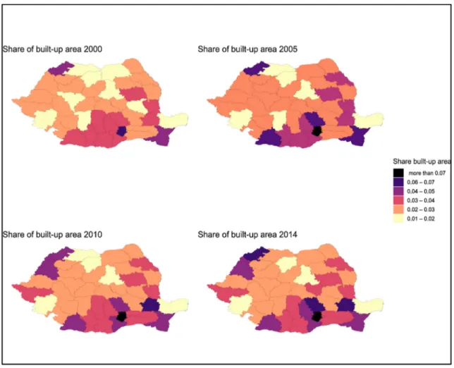
The positive and statistically significant Moran’s I highlights that areas with similar shares of residential built-up land are likely to be located close to each other. The share of residential built-up land, which is increasing over the period under analysis, means that a growing clus-terization, located in particular in the South-East where the capital city Bucharest is located and north-western parts of the country (seeFig. A1), is occurring over time. Moreover, the variance of built-up land, which, in this context provides a measure of the spatial inequality, is increasing together with Moran’s I, confirming a “polarization by nature”.
3.2. Methods
We borrow our empirical model fromBimonte and Stabile (2017a; 2017b) and we extend it in order to take account of the spatial di-mension as follows: = y + + + x + +µ y log GDP pop log GDP pop W i t t t i t i t t i , , , 2 (1) where i is the ithRomanian county of which there are n, and t is the year
of which there are T.Wtis a squared spatio-temporal spatial contiguity
weight matrix defined as the Kronecker product between the row standardized spatial weight matrix W of size n × n, and the identity matrix ITof size T, formally, Wt= IT⨂ W. W is based on a Queen
contiguity scheme, where counties are considered neighbours if they share at least one point of their borders. The parameter is the spatial autoregressive coefficient comprised between -1 and 1; µiis the vector
of spatial fixed effect (which embodies the unexplained time invariant characteristics); tis the idiosyncratic error term.
The termytrepresents the log of residential built-up area in county i at time t, while the vectorxtcomprises control variables representing
population density, the share of green areas, the number of buses over area, as a proxy for public transport, and the net migration.
In accordance with the hypothesis ofKuznets (1955), the GDP per Fig. 1. Expansion of residential built-up area and population growth in Romania.
7Moran’s I varies between the minimum and maximum eigenvector extracted from W (roughly -1 and +1). A positive (negative) value indicates positive (negative) spatial autocorrelation, i.e. locations with similar (dissimilar) values of the variable analysed are located close to each other. Moran’s I is based on a spatial weight matrix W. Formally, the spatial weights matrix is an n×n
(footnote continued)
positive matrix, where n is the number of regions. In each row i, a non-zero element wijdefines region j as being a neighbour of region i. By convention, the
capita is included non-linearly. According to his theory, GDP per capita should be concave and significantly different from zero, implying that once a certain stage of development has been reached, land use starts shrinking (Skonhoft and Solem, 2001;Culas, 2007;Liu and Guo, 2015). Equation(1)is a Spatial Lag Panel Model with spatial fixed effects (see, for instance,Elhorst, 2014). Because the model cannot be esti-mated through an Ordinary Least Squares (OLS) method, it is here es-timated with a maximum likelihood approach (ML) (Anselin, 1988a). In a standard regression model ρ = 0, i.e., Wtyt= 0, so the marginal effect
of a change in a variable belonging to vector x, say xi, would be equal to
θi. In the Spatial Lag Panel Model, the marginal impact of a change in a
regressor on the dependent variable is related not only to θibut also to
the spatial lag coefficient ρ, given that it is associated with the spatial autoregressive parameter Wtyt. The spatial lag coefficient ρ associated
with the spatial autoregressive parameter generates spill-overs due to the spatial multiplier 1/(1-ρ), whose matricial form is (I-ρW)-1and that
can be expressed as a geometric series: I+ ρW+ρ2W2+…+ρnWn.
Loosely speaking, this means that the total impact of a change in a variable xion land use is the result of the interaction among other
neighbouring counties. Indeed, following LeSage and Page (2009) the total effect of a change in xiis disentangled into two components: i) the
direct effect, which is the result of a marginal change of a variable in a certain spatial unit i on the dependent variable of the same unit i,8and
ii) the indirect effect, which corresponds to the impact that changes in the explanatory variable in a neighbour county j exert in county i due to spatial spill-overs; or, alternatively, how a shock hitting a county i, which has also an impact on the neighbour counties j, is reflected back to county i. Formally, the total impact of a change in a variable θi(its
marginal effect), is equal to the average of the values of the matrix
(I-ρW)-1θ
i, the direct effects to the average of the diagonal elements of
(I-ρW)-1θ
i, and the indirect effects to the average of the off- diagonal
elements of (I-ρW)-1θ
i.
Our selection of the Spatial Lag Panel Model is due not only to the idea that built-up land in a specific location is positively related to its use in neighbouring locations, but also to a set of statistical tests. The
Hausman test is used on standard and Spatial Lag Panel Model to de-termine if fixed or random effect has to be chosen. The selection of the Spatial Lag Panel Model is based on a Lagrange Multiplier (LM) (Anselin, 1988b;Anselin et al., 1996). LM test for spatial error depen-dence (LMerr) and LM test for spatial lag dependence (LMlag) are carried
out on the residuals of the standard (not spatial) regression. The model is selected according to the most significant test. If both are not sta-tistically significant, a non-spatial model has to be chosen. Otherwise, if both are significant, the spatial lag or spatial error model is chosen according to the most significant robust version of the two LM tests mentioned above. We additionally test for the presence of spatial au-tocorrelation on the residuals of the standard and spatial models via a randomized Moran test based on 1,000 permutations. Furthermore, for each model, we check for heteroskedasticity using the Breush-Pagan test and for model misspecification through the RESET test. Finally, multicollinearity issues are checked by means of the Variance Inflation Factor (VIF).
3.3. Data
All the variables employed in the analysis are constructed using annual data over the 2000-2014 time-period from the TEMPO dataset issued by the Romanian National Institute of Statistics. Data are dis-aggregated at NUTS3 level accounting for the 41 Romanian counties plus the capital city Bucharest. The built-up land use, i.e. our dependent variable, is expressed as the log of the share of hectares of residential built-up land in the total number of hectares of each county. The only monetary variable employed in the analysis, namely the log of per ca-pita GDP, is reported at 2005 Lei constant prices. The GDP deflator was taken from the World Bank.
To deal with potential misspecification problems, we also consider possible control variables that enter the model specification as ex-planatory (descriptive statistics are provided inTable B1in Appendix B). They are defined as follows:
•
Population density is the ratio between the population and the area inhectares of a certain county. It is a proxy for agglomeration, which is linked to geographical concentration of economic activities and raising productivity which, in turn, increases wages (Duranton and Puga, 2003;Charlot and Duranton, 2004). On the other hand, po-pulation concentration, since it is expected to increase the Fig. 2. Gini and Moran’s I of the residential built-up land.
8The direct effect accounts also for the feedback effects that, in general, are sizable. According toLeSage and Pace (2009: 36), “These arise because region i is considered a neighbour to its neighbour, so that impacts passing through neighbouring regions will exert a feedback influence on region i itself.”
residential land consumption, may impose high pressure on the housing market, increasing prices and potentially off-setting the rising wages. Both processes can modify peoples’ location choices (World Bank, 2013).
•
Share of green areas is expressed as the percentage of hectares of landdevoted to public parks and green spaces over the total number of hectares of each county. This is a proxy for the presence of natural and environmental amenities in an area (Borgoni et al., 2018; Schaeffer and Dissart, 2018). Previous studies on Romania highlight that the access to public open spaces and parks can be associated with sustainable urban planning strategy (Badiu et al., 2016);
•
Number of buses over area (in hectares) is considered a proxy for thepublic transport system because the bus is by far the most used public means of transport. Indeed, according to Eurostat data, be-tween 2000 and 2014 passengers using buses increased from 12.2% to 16.9% while, over the same period, train transport decreased from 16.3% to 4.6%.9The presence of public transport has a positive
effect on house prices because people are disposed to pay more for being close to the service (Des Rosiers et al., 2010; Wang et al., 2015). This, in turn, may be an incentive to increase the urbanised area, or to convert low density areas into higher density places, as shown, for example, byCervero and Kang (2011). Heavy reliance on public transport and better connectivity are more likely to be ob-served in higher urban densities areas like compact and dense cities (Lehmann, 2008,Newman and Kenworthy, 1989);
•
Net migration over population is the balance between immigrationand emigration flows with respect to the total population. Inbound (outbound) migration flows can increase (decrease) the housing demand (Bell et al., 2010) and leave space for speculation due to the rising rent prices (Saiz, 2003,2007). Out-migration, on the other hand, can determine inflows of remittances that can be used for consumption or investment (Yang, 2011). Although there is em-pirical evidence that remittances are used mainly for consumption and only secondarily for investment (see, among others, Chami et al., 2003), we cannot exclude that they have a significant effect on real estate. However, unfortunately, we cannot empirically control the effect of remittances on residential built-up land because the Romanian National Institute of Statistics does not provide data on remittances at county level.
4. Results
In our empirical estimation we proceed as follows. The first phase is estimation of a standard fixed effect panel regression model, which is chosen according to the Hausman test; in the second phase we control for the presence of spatial autocorrelation in the residuals and, if pre-sent, an appropriate spatial model (spatial lag or spatial error) is se-lected; the last step consists in estimation of the appropriate spatial model. Eq.(1)is estimated keeping our core variables, GDP per capita and its square, and then adding step by step one at a time the control variables. This enables us (i) to check for the robustness of the coeffi-cients associated with GDP per capita and its square to the inclusion of additional controls, and (ii) to identify if the latter additional controls have a significant impact too on land use. Finally, as mentioned in Section3.2, a set of tests are carried out on the estimates to check for their goodness and for the properties of the residuals.
The estimates of the standard fixed effects panel regression model are set out inTable 1and show a clear convex relation between GDP per capita and residential built-up area, even when controlling for addi-tional regressors. Nevertheless, the Breush-Pagan test reveals
heteroskedasticity of residuals and the RESET test model misspecifica-tion. On the other hand, VIF does not show multicollinearity issues. The randomized Moran test, based on 1,000 permutations, on the residuals of standard fixed effects panel regression model is statistically sig-nificant, pointing to the presence of spatial autocorrelation. Further-more, the LM test for spatial error dependence and the LM test for spatial lag dependence are both significant, and their robust versions point to spatial lag, since the Robust LM test for spatial lag dependence is more significant than the Robust LM test for spatial error dependence. Results obtained from the fixed effect Spatial Lag Panel Model are reported inTable 2. Tests on residuals show a strong improvement of the fit in terms of the Akaike Information Criterion (AIC) and residuals’ properties. Indeed, the difference between the AIC of the corresponding standard and spatial models, inTables 1 and 2, respectively, is almost always greater than around 10 or more, pointing to a “strong” pre-ference for spatial models, following the rule of thumb ofBurnham and Anderson (2004). Furthermore, in addition to the absence of spatial autocorrelation (The Moran’s I test is not significantly different from zero), also heteroskedasticity is absent, while the RESET test indicates possible non-linearities due mainly to population density.
Given these results and the considerations listed above, we focus on the estimates obtained through the fixed effect Spatial Lag Panel Model in commenting on the regression results.
The relation between GDP per capita and residential built-up land is convex ( <0; >0), and not concave as expected from the theory, implying that higher levels of land use occur for higher levels of wealth; i.e. the turning point where greater wealth implies decreasing built-up land is not reached.10This is clearly shown inFig. 3, where the log of GDP
per capita and the log of the share of built-up area are distributed along the x-axis and y-axis, respectively. The dots represent the counties and the black line the fitted (quadratic) regression line. The grey areas around the black line are the five percent confidence intervals. We can observe that the curve is relatively flat for very low values of (log) GDP per capita and then it starts growing exponentially. The 45-degree red (dashed) line can be taken as a reference for understanding at which point the elasticity of built-up land is equal to one, i.e. a 1% increase in GDP per capita implies a 1% increase in land use. We see that this happens for comparatively high levels of GDP per capita. Furthermore, it is worth mentioning that we checked for the existence of further turning points adding the third power of log(GDP/pop), finding a non-significant coefficient.
In our case, differently from the last studies listed above, as men-tioned, four additional control variables were considered to deal with misspecification issues that might arise.
The convex relation between residential built-up land and per capita GDP is confirmed when additional explanatory variables are included. The strongest and most statistically significant relationship of built-up land is with population density and natural amenities, both of which have a positive impact. Overcrowding phenomena tend to foster urba-nization, but at a decreasing rate, while the proximity of public green parks, which in principle can be associated with sustainable urbaniza-tion, has also the effect of attracting speculation. The proxy for public transport is positive and marginally statistically significant, and the proxy for net migration is positive but not statistically significant. The effect of the latter, in particular, can be explained by the evidence that despite persistently heavy outflows in Romania during the period under analysis (Eurostat, 2011),11 residential built-up land was still very
9Since, according to the Global Competitiveness Report 2018 (Schwab,
2018), railroad efficiency is very low in Romania, ranking the country in 2018 24thout of 26 EU countries for which data were available, we consider the bus transport a valid proxy.
10These findings, as happens in the literature, are based on an empirical regularity drawn from existing data that provide a snapshot of the present si-tuation. In our study, indeed, we are not able and we do not aim to forecast if, in the future, further turning points in terms of GDP could be reached, which is reasonable in a developing country like Romania.
11During the period from 2001 to 2010, people left Romania to work abroad and became the group of non-nationals living in the EU with the largest increase (almost seven-fold from 0.3 million in 2001 to 2.1 million by 2010).
intense, as shown also inFig. 1.
Inspection ofTables 1 and 2shows that the values of the regression coefficients estimated with standard panel models are bigger in size than the ones estimated with the Spatial Lag Panel Model because
spatial dependence is not correctly modelled. This happens because, as in an a-spatial regression ρ = 0, spatial dependence is implicitly em-bedded in the dependent variable, causing upward biased regression coefficients. The Spatial Lag Panel Model, compared with the standard Table 1
Panel Estimates for residential built-up area.
(1) (2) (3) (4) (5) (6) (7) (8) Log(GDP/pop) −1.776 *** −1.3925 *** −0.8146 *** −1.7895 *** −1.7864 *** −1.7809 *** −1.5274 *** −1.0132 *** (0.2912) (0.2813) (0.2770) (0.2849) (0.2870) (0.2905) (0.2966) (0.2907) Log(GDP/pop)2 0.1099 *** 0.0884 *** 0.0567 *** 0.1106 *** 0.1104 *** 0.1100 *** 0.0960 *** 0.0679 *** (0.0162) (0.0156) (0.0154) (0.0159) *** (0.0160) (0.0162) (0.0165) (0.0162) Pop. density 0.2949 *** 1.0201 *** 0.3112 *** 0.9904 *** (0.0603) (0.1074) (0.0058) (0.1085) Pop. density2 −0.0056 *** −0.0055 *** (0.0007) (0.0007) Green areas 3.7883 ** 4.9200 ** 3.0883 * (1.7395) (1.7445) (1.6541) Buses/area 7.2968 * −0.2945 4.9035 (3.9956) (4.1219) (4.0759) Net migr./pop. 6.0668 * 4.5501 1.9518 (3.3768) (3.3018) (3.0745) Turning point 3229 2634 1317 3262 3264 3278 2850 1739 Observations 630 630 630 630 630 630 630 630 R squared (adj.) 0.3196(0.3174) 0.3667(0.3191) 0.4290(0.3850) (0.2970)0.3462 0.3446(0.2953) 0.3233(0.3200) 0.3777(0.3275) 0.4593(0.4532) AIC −1308.98 −1332.21 −1401.51 −1312.07 −1310.56 −1310.53 −1337.25 −1395.51 Moran’s I 0.04779 ** 0.0590 ** 0.0990 *** 0.0365 * 0.0576 ** 0.0387 * 0.0385 * 0.0856 *** LM spatial lag 10.2674 *** 11.0095 *** 15.7604 *** 9.8322 *** 12.4014 *** 9.1203 *** 9.3583 *** 17.1145 *** LM spatial error 3.2333 4.9324 ** 13.8667 *** 1.8322 4.6930 ** 2.1203 2.1042 10.3680 *** Robust LM spatial lag 20.1480 *** 11.7751 *** 2.4670 29.8307 *** 18.3984 *** 23.1812 *** 21.1327 *** 7.0379 *** Robust LM spatial error 13.1139 *** 5.6981 ** 0.5733 21.8871 *** 10.6900 *** 16.2492 *** 13.8786 *** 0.2913 Hausman test 2.6973 18.621 *** 18.621 *** 20.282 *** 39.944 *** 2.7251 19.53 *** 65.463 *** Reset test 6.06
(p-val = 0.01) 21.04(p-val<0.01) 4.49(p-val = 0.03) 3.73(p-val = 0.05) 3.614(p-val = 0.06) 5.36(p-val = 0.021) 16.67(p-val<0.01) 1.51(p-val = 0.21) Breusch-Pagan test 172.23
(p-val<0.01) 21.75(p-val<0.01) 2.57(p-val = 0.63) 23.49(p-val<0.01) 23.49(p-val<0.01) 181.6(p-val<0.01) 25.69(p-val<0.01) 8.43(p-val = 0.30)
VIF 1.517 1.579 1.7514 1.529 1.529 1.526 1.607 1.7683
Note: *p ≤ 0.05; **p ≤ 0.01; ***p ≤ 0.001. Std. errors in parenthesis. Turning point is calculated as the exponential of the coefficient of Log(GDP/pop) over two
times the coefficient of Log(GDP/pop)2. Prices are expressed at 2005 Lei constant prices.
Table 2
Spatial Panel Estimates for residential built-up area.
(9) (10) (11) (12) (13) (14) (15) (16) Log(GDP/pop) −1.4827 *** −1.1977 *** −0.5521 ** −1.5987 *** −1.5983 *** −1.4981 *** −1.3724 *** −0.7658 *** (0.2687) (0.2489) (0.2631) (0.2725) (0.2738) (0.2681) (0.2828) (0.2750) Log(GDP/pop)2 0.0917 *** 0.0759 *** 0.0400 *** 0.0984 *** 0.0981 *** 0.0926 *** 0.0859 *** 0.0520 *** (0.0149) (0.0149) (0.0146) (0.0152) (0.0152) (0.0149) (0.0158) (0.01531) Pop. density 0.2955 *** 1.0448 *** 0.3026 *** 1.0182 *** (0.0577) (0.0102) (0.0621) (0.1026) Pop. density2 −0.0058 *** −0.0059 *** (0.0007) (0.0007) Green areas 3.6307 ** 4.7613 *** 2.7584 * (1.6638) (1.6367) (1.5647) Buses/area 8.9540 ** 1.4414 7.6421 ** (3.8131) (4.0189) (3.8557) Net migr./pop. 5.1510 * 3.6565 5.4664 (3.1149) (3.0557) (2.9084) Turning point 3244 2670 993 3373 3451 3259 2946 1577 Rho 0.1305 *** 0.1329 *** 0.1602 *** 0.1272 *** 0.1462 *** 0.1234 0.1260 *** 0.1767 *** (0.0470) (0.0465) (0.0454) (0.0470) (0.0473) (0.0473) (0.0469) (0.0454) Observations 630 630 630 630 630 630 630 630 AIC −1318.50 −1342.22 −1410.92 −1321.24 −1321.88 −1319.20 −1346.27 −1412.21 Moran’s I −0.0438 −0.0336 0.0076 −0.0511 −0.0424 −0.0462 −0.0439 0.0069 Hausman test 41.765 *** 37.519 *** 110.27 *** 92.841 *** 39.358 *** 41.929 *** 55.837 *** 82.246 *** Reset test 0.44
(p-val. = 0.64) 22.03(p-val<0.01) 1.64(p-val = 0.16) 0.87(p-val = 0.45) 2.44(p-val = 0.06) 1.74(p-val = 0.16) 14.01(p-val<0.01) 3.619(p-val<0.01) Breusch-Pagan test 5.39
(p-val = 1) 0.22(p-val = 0.97) 4.42(p-val = 0.1) 5.30(p-val = 1) 4.58(p-val = 1) 5.80(p-val = 1) 5.66(p-val = 1) 3.8819(p-val = 1)
VIF 1.517 1.579 1.7514 1.529 1.526 1.526 1.607 1.7683
Note: *p ≤ 0.05; **p ≤ 0.01; ***p ≤ 0.001. Std. errors in parenthesis. Turning point is calculated as the exponential of the coefficient of Log(GDP/pop) over two
panels, enables us to estimate also the direct, indirect and total effects due to the spatial multiplier. The direct, indirect and total effects based on the Spatial Lag Panel Model are reported in Table 3and refer to model (16) inTable 2.
The values of the direct effects are in line with the coefficient esti-mates, while the total effects are around 21% larger because they in-corporate the indirect effects due to the spatial multiplier, obtained as 1/(1−ρ). In the case of model (16) in Table 2, it is equal to 1/(1-0.177) = 1.21. Residential built-up land in a certain county i is de-termined jointly by the stage of development of the county in which it is located and the surrounding counties. This phenomenon, namely spa-tial spill-over, can be explained by the fact that, as wealth increases in these neighbourhoods, people may decide to invest not only where they live, but also in the neighbouring counties, thus increasing their built-up land. Analogously, a shock hitting the available income in one county has repercussions in the real estate market of the neighbouring counties, and back to the first one through the spatial multiplier.
Finally, mention should be made of LeSage and Pace’s study (2009), which introduced a partitioning technique that can be used to compute the coefficient estimates by different orders of neighbours, determining their relative importance in explaining residential built-up land. The results of this analysis, available upon request, show that spatial spil-lovers are confined to the immediate neighbour. This is reasonable given our units of observation, and demonstrates not only that what happens in a county is not independent from what happens in neigh-bouring counties, but also that the phenomenon of polarization and of “clusterization in nature” observed inFig. 2 and Fig. A1in Appendix A holds also when we control the built-up land dimension. This has major policy implications that will be discussed in the following section.
To better understand the residential built-up land dynamics, the estimates are replicated by considering as dependent variable the city size as proxied by the share of hectares of urban area on the total
number of hectares of each county.12The results, set out inTables C1
and C2in Appendix C, are close to those inTables 1 and 2, indicating not only that built-up area and city growth are closely related (the correlation between them is 0.85) but also that, specifically, these Fig. 3. Marginal effect of GDP per capita over residential built-up land based on model (16).
Table 3
Direct, Indirect and Total Effects Estimates.
direct indirect total Log(GDP/pop) −0.7711 *** −0.1590 ** −0.9302 *** (-2.7300) (-2.1042) (-2.7118) Log(GDP/pop)2 0.0523 *** 0.0108 ** 0.0631 *** (3.3427) (2.3484) (8.7259) Population density 1.0253 *** 0.2114 *** 1.2367 *** (10.1004) (3.0602) (8.7259) Population density2 −0.0059 *** −0.0012 *** 0.0071 *** (-8.9614) (-2.9681) (-7.8249) Share of green areas 2.7777 * 0.5728 3.3503 *
(1.8011) (1.5655) (1.8061) Number of buses over area 7.6951 * 1.5870 * 9..2820 *
(1.9295) (1.6771) (1.9371) Net migration over pop. 0.5504 0.1135 0.6639
(0.2848) (0.2567) (0.2819)
Note: *p ≤ 0.05; **p ≤ 0.01; ***p ≤ 0.001. Z-values based on 1000
permuta-tions in parenthesis for the direct, indirect and total effects in parenthesis. Estimates are based on model (16) inTable 2.
12According to the indicator “GOS102A - Inside town area of municipalities and towns by counties and localities”, of the TEMPO database, “The built-up area (ha) represents the territorial area comprised in the buildable perimeter of municipalities and towns, including the localities belonging to municipalities and towns, according to the systematisation plan approved for that locality. The area of villages which belong to the municipality (the town) is not included.”
findings confirm whatIațu and Eva (2016)found, i.e. that in Romania the increase of built-up areas coincides with city expansion and its suburbanization. In this regard,Ionescu-Heroiu et al. (2014: 40)show that the development patterns of new housing units from 1990 to 2011 confirm that the Romanian population is concentrating around key economic centres, including suburban areas that may offer better living standards at a more affordable price. Suburbs around major cities gained around 300,000 inhabitants between the 1990 and 2011 Cen-suses, while the country’s total population decreased by 4 million people. The suburbanization process, according to Sýkora and Ouředníček (2007), affects the spatial distribution of the population and increases inequalities (Petrovici, 2012). Indeed, contrary to the traditional socio-spatial patterns of the socialist cities, suburban zones are now characterized by élite persons with high incomes (Ouředníček, 2007), causing social tensions and residential segregation (Soós and Ignits, 2003) in territories traditionally populated by the working class and inhabitants of the former rural settlements.
Finally, it is worth mentioning that, as a robustness check, we es-timated both models (standard and spatial) by means of random effects, and the results hold.
5. Discussion
In light of the main results of the analysis, we discuss the potential causes behind land use dynamics in Romania and identify a role for policy interventions. Our first main finding demonstrates that there is a convex relation between economic development and residential built-up land, which contrasts with the classic inverted U-shape predicted by the EKC. This outcome, despite its contrast with some recent empirical analyses conducted on the relation between income and environmental variables (see, among others,Skonhoft and Solem, 2001;Culas, 2007; Liu and Guo, 2015), is not an isolated case in Europe, because it has been found byBimonte and Stabile (2017a;2017b) for Italy. Differently from previous studies, however, we extend the classic EKC framework to include spatial effects explicitly, which yield useful information that enables us to draw additional policy implications.
In the Romanian case, the increasing marginal effects of GDP per capita on residential built-up land and thus on city expansion can be explained by various alternative factors.
One of them is the weak institutional framework and the lack of transparency of the public administration (data from Worldwide Governance Indicators) and contradictory policies that have made land speculation possible (Niţă et al., 2015).Tudor et al. (2015), indeed, show that the land-use regulation has been not properly implemented in recent years, leading to an increased likelihood of distressed situa-tions (Iojă et al., 2014;Tudor et al., 2013). According toBTI (2018: 26), “the central government has used various mechanisms and legal loop-holes to prevent local government from actually increasing its leeway or making autonomous decisions in a large number of policy fields. On the other hand, many local decisions, taken in the previous climate of loose budget constraints, were clientelistic or simply wasteful”. Local authorities took advantage of urban sprawl as a way to increase their budgets through new taxation areas (Suditu, 2012). The resulting spa-tial pattern, as observed bySýkora and Ourednek (2007)contrasts with the compact built-up areas developed during the communist period. This increased land speculation leads to urban fragmentation (Hirt, 2013). Furthermore, agricultural land abandonment, which char-acterised Romania after the transition (Kuemmerle et al., 2009), has been proved to be a precursor of built-up development at the sprawling peripheries (Grădinaru et al., 2015a) that compromise the sustainable development of the urban landscape as long as urban planning is not under control and the collaboration among authority levels is rather weak (Grădinaru et al., 2015b).
Another interpretation of our results is that the transition in the past two decades from a centrally planned structure to a decentralised one, and the EU accession in 2007, have resulted in a complex regulatory
framework. During this process, several land laws13 have been
pro-mulgated to discipline decollectivisation and privatisation of the pre-vious state-owned land since the first law No 18/1991 also known as “The Land Law”, and the national land policy has been harmonized with the Common Agricultural Policy (CAP) prescriptions. As a con-sequence of both the switch from the state to a private regime and the convergence on EU criteria, local governments have experienced an even greater knowledge lag about the quality of individual properties, including the property rights, thus facing huge urban planning and management challenges. Information asymmetry may arise between economic agents with local administrations that may find it convenient to grant additional building permits to maximise their revenues at the expense of an excessive and unsustainable urban development (Suditu, 2012). Furthermore, the positive and significant spatial lag, which ac-counts for the second main result of the analysis, can be interpreted as evidence of policy mimicking among neighbours, as found for example byRevelli (2001)in the UK context. This implies that, with the aim of not leaving all the advantages of additional revenues from granting building permits to the neighbouring governments, local governments of a certain county may grant higher “urbanistic freedom” in response to the neighbours’ behaviour. Private agents, on the other hand, might find it preferable to behave like their counterparts in the neighbouring counties so as not to leave them all the advantages of the rising real estate prices. These results extend the win-win game observed for Italy byBimonte and Stabile (2017a;2017b), where public and private in-terests, together with institutional and political elements, interact in a spatial context.
An additional result of the analysis is the robustness of the existence of a convex relation between residential built-up land and per capita GDP to the inclusion of additional explanatory variables, namely po-pulation density, natural amenities, public transport and net migration. Therefore, in what follows, the discussion will focus upon those factors and their different roles in affecting the residential built-up pattern.
Regarding the effect of population density, a possible interpretation of the mechanisms responsible in Romania for its positive relation with the extensive built-up land use can be, as documented by theWorld Bank (2013), the fact that population distribution in major cities fol-lows what is known as a ‘camel-back’ pattern, i.e. a city’s periphery has a higher population density than the central business district. This is related to the post-communist suburban residential preferences that led to the increasing urbanization of suburban municipalities adjacent to major cities (Ionescu-Heroiu et al., 2014) due to the inability to re-configure the fixed capital stock of central cities, driving a very rapid rate of expansion of major Romanian cities (World Bank, 2013). Fur-thermore, the lack of policy vision and planning of the local public administration has contributed to generating chaotic and unsustainable sprawl, prioritizing private financial profits rather than public interest (Nae et al. 2019). This process has been due to the mass privatization (Buckley and Mathema, 2017) supported by the financial sector. In Romania, indeed, monthly mortgage payments are equal to, or even lower than, monthly rental payments, pushing up the homeownership rate contributing to suburbanization (Grigorescu et al., 2012b;Iațu and Eva, 2016).14Romanian banks offer a special credit that is guaranteed
by the Government, which in 2009 launched the First Home program to restart mortgage lending and support the construction sector in the aftermath of the financial crisis (Government Urgency Ordinance no.
13Among several laws (No 15/1990, No 31/1990, No 169/1997, No 1/2000) that influenced the land changes, the more recent No 198/1999 and No. 46/ 2000 were legislated to reorganize the state-owned farms into private trading companies.
14According to Eurostat, Romania has the highest homeownership rate in Europe in 2016. About 96% of Romanians own their residential properties. Moreover in 2016 the highest rate of people living in overcrowded dwellings among the Member States was registered in Romania (48.4%), followed by Latvia and Bulgaria.
60/2009 and Government Decision no. 717/2009).
The positive and statistically significant coefficient associated with the intrinsic value of natural and environmental amenities may be as-sociated with their scarcity (Suditu et al., 2004) due to the transition process that came at the expense of the conversion of green and agrarian landscapes into built-up land with industrial and residential uses. This is demonstrated by the fact that, in light of their importance, and given that in Romania environmental changes are the catalyst for land-use conflicts (Ianos et al., 2012), as a consequence of the EU ac-cession, a sustainable urban policy process has been framed. Indeed, currently, to comply with the EU Policy on urban environment as stated by the 7th Environmental Action Programme (7EAP) under the Priority Objective 8 on Sustainable Cities, in 2006 the Romanian government promulgated law no. 265/2006 for the environmental protection of soil through adequate interventions of management and conservation.
Regarding the positive effects of the variable that proxies public transport, to be noted is that, according to the World Bank (2013), public transport provision is crucial in Romania given that uncontrolled urban expansion due to planning fragmentation has increased pressures on transport infrastructure and utilities. However, public transport provision, because people are disposed to pay more for housing located near easily accessible services, may push up the residential built-up land use and urban expansion (seeCervero and Kang, 2011).Towards the end of the 1990s, Romania started to receive support to strengthen its public transport system from the European Bank for Reconstruction and Development and international donors. Thereafter, from 2007, the EU structural funds contributed to subsidising the process. The policy objective to create an integrated transport network, given that the private car is the prevalent means of transport in the country (Iordache, 2009and Eurostat data), is now even more urgent as urban sprawl is likely to increase (Iațu et al., 2011). However, since public transport plays an important role in city expansion, fares should be kept at market level because, if artificially low, they could lead to unsustain-able (sub)urban development patterns that incentivize, for example, commuting from the suburbs instead of living closer to the city centre (World Bank, 2013).
Finally, the coefficient of net migration is found not to be sig-nificant. Considering that Romania is losing population, the net out-flows may impact indirectly on the residential built-up land use through the role of remittances for real estate purposes. Indeed, as observed by Mehedintu et al. (2020), in Romania, people’s decreasing intention to engage in productive activities, relying on remittances, and the rise of inflationary pressure due to the excessive demand for land and houses caused by the artificial increase of their prices may be listed among the possible negative effects of remittances. In our study, however, the unavailability of data on remittances prevents us from investigating further the lack of significance of our variable, which might be due to the fact that (i) it does not proxy remittances well, or that (ii) re-mittances do not have the foreseen impact.
In view of the SDGs on socially sustainable spatial planning and of the EU Urban Partnership and the New Urban Agenda, the empirical evidence presented in this paper suggests various possible policy in-terventions. A first concern consists not only in the need to strengthen the institutional framework, to design an accessible and transparent cadastral system, and close the housing legislation lag, but also to re-think the main channel through which local governments collect their revenues, lowering the importance of property taxes. Another option, aimed at limiting real estate speculation, is to improve the legal rent control with more severe protection measures for the parties and to
provide incentives for restructuring houses rather than building new ones. This last point, framed in a wider context of urban regeneration, would improve living standards in cities and suburbs, mitigating the rise of house prices in order to respect habitat preservation. A more flexible approach to land-use planning recommended by the OECD (2017)requires co-ordination across all levels of government as well as across policy domains, to be timelier and adaptable to new challenges. Accordingly, horizontal policies like transport policy, environmental and building code regulations, spatial framework plans and population mobility have to be integrated with each other and, as demonstrated in our paper, coordinated among neighbours to avoid freeriding behaviour and to promote sustainable development.
6. Conclusions
In this paper, we have analysed the relationship between GDP per capita and residential built-up land among Romanian NUTS3 regions.
Romania is an interesting case study not only per se, as it is little explored in the literature, but also because it is one of the poorest EU member states, that could be taken as a reference to analyse similar contexts. Besides the convex relation between residential built-up land and economic development, the relation between city size and eco-nomic development has also been considered, leading to the conclusion that the mass residential built-up land expansion in Romania mainly reflects the process of city expansion and urbanization phenomena such as sprawl or suburbanization. Generally speaking, however, although the EKC, even with the explicit inclusion of spatial spill-overs, is a tool easily applicable and understandable, it is not always possible to model the factors affecting the land use conversion because they differ among countries, among regions, and over time even within a single country. In the context of the EKC for residential built-up land, our study, like similar studies in the literature, has relied on a relatively short time span, due to data limitation. However, to assess the general validity of the EKC for residential built-up land, an extension using longer time series is required in the future. Furthermore, our approach to the EKC reveals its limitation, because prescriptions in terms of the environ-mental impact of excessive land use cannot be drawn directly from its analysis per se; rather, they require a literature overview that indirectly allows one to infer the negative implications for the environment of the suburbanization process and sprawling phenomena. In our context, the geography of inequalities, the role of migration flows and remittances, which contribute to explaining how population distributed in the urban space in the post-socialism period, their causal relation with the built-up land consumption and the social and environmental consequences deserve further attention. Finally, another aspect that warrants in-vestigation in the future is the effect of the state-to-private regime switch and its consequences in terms of intensive spatial urban/sub-urban development among the Central and South-Eastern European states.
Authors statement
The authors contributed equally to this work. Acknowledgements
The authors thank two anonymous reviewers for their valuable feedback.
Appendix A
Appendix B
Fig. A1. Residential built-up land over the 2000-2014 period by NUTS3.
Table B1
Descriptive statistics.
Variable Min. Mean Max. Std. Dev.
Log(Share built-up area) −4.6388 −3.5070 −0.4081 0.6176
Log(Share area occupied by
cities) −5.5540 −4.1760 −4.000 0.8086
Log(GDP/pop) 7.8800 9.0790 10.4360 0.4210
Population density 0.2920 3.0296 90.8860 13.6843
Share of green areas 0.00008 0.0051 0.2034 0.0286
Number of buses over area 0.000009 0.0015 0.0651 0.0085
Appendix C
Table C1
Panel Estimates on city size.
(1a) (2a) (3a) (4a) (5a) (6a) (7a) (8a)
Log(GDP/pop) −1.6796 *** −1.7029 *** −0.4096 −2.0578 *** −1.6771 *** −1.9155 *** −1.4925 *** −0.7195 (0.4652) (0.4661) (0.4652) (0.4665) (0.4768) (0.4817) (0.4891) (0.4838) Log(GDP/pop)2 0.1174 *** 0.1189 *** 0.0474 * 0.1389 *** 0.1172 *** 0.1309 *** 0.1073 *** 0.0650 ** (0.0259) (0.0259) (0.0259) (0.0260) (0.0265) (0.0268) (0.0273) (0.0269) Pop. density 0.0399 *** 1.5238 *** 0.4730 *** 1.4939 *** (0.0045) (0.1804) (0.1073) (0.1805) Pop. density2 −0.0091 *** −0.0083 *** (0.0012) (0.0012) Green areas 12.3596 *** 13.8868 *** 11.1336 *** (2.8483) (2.8303) (2.7525) Buses/area −0.1587 −10.6507 −2.8377 (6.6391) (6.9496) (6.7824) Net migr./pop. 4.7273 3.5396 −0,3658 (5.6027) (5.2841) (5.1160) Turning point 1278 1288 – 1648 1280 1505 1048 – Observations 630 630 630 630 630 630 630 630 R squared (adj.) 0.4490(0.4086) 0.4848(0.4833) 0.5097(0.4719) (0.42604)0.4662 0.4490(0.4076) 0.4298(4.7273) 0.4841(0.4792) 0.5232(0.4838) AIC −672.754 −684.047 −710.27 −690.712 −670.755 −671.551 −706.269 −704.269 Moran’s I 0.0487 ** 0.0488 ** 0.1114 ** 0.0912 *** 0.0486 ** 0.0592 ** 0.0161 0.1583 *** LM spatial lag 7.1896 * 6.0040 ** 18.6343 *** 18.5237 *** 7.1764 *** 7.0383 *** 11.8000 *** 34.8632 *** LM spatial error 3.3558 *** 2.6471 * 17.5724 *** 11.8000 *** 3.3418 * 3.2442 * 18.5237 *** 35.4772 *** Robust LM spatial lag 7.0323 * 6.2242 ** 2.1008 8.3864 *** 7.0571 *** 7.0467 *** 1.6628 2.4774 Robust LM spatial error 7.0323 *** 2.8672 ** 1.0389 1.6628 3.2225 * 3.2526 * 8.3864 *** 3.0914 * Hausman test 7.4798 ** 4.566 44.823 *** 14.458 *** 43.104 ** 7.4931 * 15.64 ** 50.88 *** Reset test 6.06
(p-val. = 0.01) 24.72(p-val<0.01) 5.777(p-val = 0.01) 67.72(p-val<0.01) 1.98(p-val = 0.160) 1.85(p-val = 0.175) 0.43(p-val = 0.51) 14.94(p-val<0.01) Breusch-Pagan test 192.82
(p-val<0.01) 46.45(p-val<0.01) 12.72(p-val = 0.01) 51.79(p-val<0.01) 46.80(p-val<0.01) 195.83(p-val<0.01) 45.18(p-val<0.01) 17.72(p-val = 0.01)
VIF 1.815 1.854 2.039 1.873 1.815 1.817 1.938 2.097
Note: *p ≤ 0.05; **p ≤ 0.01; ***p ≤ 0.001. Std. errors in parenthesis. Turning point is calculated as the exponential of the coefficient of Log(GDP/pop) over two
times the coefficient of Log(GDP/pop)2. Prices are expressed at 2005 Lei constant prices.
Table C2
Spatial Panel Estimates on city size.
(9a) (10a) (11a) (12a) (13a) (14a) (15a) (16a)
Log(GDP/pop) −1.5718 *** −1.5351 *** 0.0013 −1.9104 *** −1.4917 *** −1.5782 *** −1.8780 *** −0.3432 (0.4617) (0.4612) (0.4417) (0.4508) (0.4573) (0.4615) (0.4720) (0.4512) Log(GDP/pop)2 0.1089 *** 0.1075 *** 0.0202 0.1266 *** 0.1043 *** 0.1091 *** 0.1251 *** 0.0379 (0.4617) (0.0257) (0.0245) (0.0251) (0.0255) (0.0257) (0.0263) (0.0251) Pop. density 0.0391 *** 1.6119 *** 0.0066 *** 1.6057 *** (0.0048) (0.1713) (0.0089) (0.1683) Pop. density2 −0.0099 *** −0.0095 *** (0.0011) (0.0011) Green areas 16.8302 *** 14.6951 *** 15.4915 *** (1.7952) (2.7765) (2.5671) Buses/area 1.1075 1.4544 2.8809 (6.3677) (6.5602) (6.3256) Net migr./pop. 4.3297 4.0807 −1.9299 (5.3639) (5.2542) (4.7715) Turning point 1362 1261 – 1891 1275 1384 1819 – Rho 0.1013 ** 0.0758 * 0.1610 * 0.1627 *** 0.0959 ** 0.1002 ** 0.1497 *** 0.2407 *** (0.0448) (0.0445) (0.0425) (0.0436) (0.0442) (0.0446) (0.0462) (0.0436) Observations 630 630 630 630 630 630 630 630 AIC −679.385 −689.898 −758.251 −707.540 −677.415 −678.082 −721.586 −784.637 Moran’s I 0.2127 *** −0.0336 −0.0396 −0.0095 −0.0272 0.2119 *** −0.0595 −0.0313 Hausman test 4.0319 6.1865 6.1865 6.1078 28.742 *** 0.5619 13.045 * 22.772 *** Reset test 0.10
(p-val = 0.90) 19.47(p-val<0.01) 2.84(p-val = 0.02) 19.47(p-val<0.01) 0.37(p-val = 0.78) 3.08(p-val = 0.027) 11.30(p-val<0.01) 3.76(p-val<0.01) Breusch-Pagan test 24.27
(p-val = 0.99) 28.61(p-val = 0.96) 9.21(p-val = 1) 28.61(p-val = 0.96) 24.61(p-val = 0.99) 24.01(p-val = 0.99) 8.70(p-val = 1) 4.91(p-val = 1)
VIF 1.815 1.854 2.039 1.873 1.817 1.815 1.938 2.097
Note: *p ≤ 0.05; **p ≤ 0.01; ***p ≤ 0.001. Std. errors in parenthesis. Turning point is calculated as the exponential of the coefficient of Log(GDP/pop) over two
Appendix D. Supplementary data
Supplementary material related to this article can be found, in the online version, at doi:https://doi.org/10.1016/j.landusepol.2020.104695. References
Alberti, M., 2005. The Effects of Urban Patterns on Ecosystem Function. International Regional Science Review 28, 168–192.
Anselin, L., 1988a. Spatial Econometrics: Methods and Models. Kluwer Academic Publishers, Dordrecht.
Anselin, L., 1988b. Lagrange multiplier test diagnostics for spatial dependence and spatial heterogeneity. Geographical Analysis 20, 1–17.
Anselin, L., Bera, A., Florax, R., Yoon, M., 1996. Simple diagnostic tests for spatial de-pendence. Regional Science and Urban Economics 26, 77–104.
Badiu, L.D., Iojă, C.I., Pătroescua, M., Breuste, J., Artmann, M., Nită, M.R., Grădinaru, S.R., Hossua, C.A., Onosea, D.A., 2016. Is urban green space per capita a valuable target to achieve cities’ sustainability goals? Romania as a case study. Ecological Indicators 50, 53–66.
Bell, S., Alves, S., Silveirinha de Oliveira, E., Zuin, A., 2010. Migration and Land Use Change in Europe: A Review. Living Review in Landscape Research 4, 2.
Bimonte, S., Stabile, A., 2017a. EKC and the income elasticity hypothesis Land for housing or land for future? Ecological Indicators 73, 800–808.
Bimonte, S., Stabile, A., 2017b. Land consumption and income in Italy: a case of inverted EKC. Ecological Economics 131, 36–43.
Borgoni, R., Michelangeli, A., Pontarollo, N., 2018. The value of culture to urban housing markets. Regional Studies 52 (12), 1672–1683.
Bertelsmann Stiftung’s Transformation Index, 2018. BTI 2018 Country Report: Romania (retrieved from:https://www.bti-project.org/fileadmin/files/BTI/Downloads/ Reports/2018/pdf/BTI_2018_Romania.pdflast access 15 December 2019). .
Buckley, R., Mathema, A., 2017. Housing privatization in Romania· An Anti‐commons tragedy? Economics of Transition and Institutional Change 26, 127–145.
Burnham, K.P., Anderson, D.R., 2004. Multimodel Inference: Understanding AIC and BIC in Model Selection. Sociological Methods and Research 33, 261–304.
Cervero, R., Kang, C.D., 2011. Bus rapid transit impacts on land uses and land values in Seoul, Korea. Transport Policy 18, 102–116.
Chami, R., Fullenkamp, C., Jahjah, S., 2003. Are immigrant remittance flows a source of capital for development? IMF Working Papers, WP/03/189..
Charlot, S., Duranton, G., 2004. Communication externalities in cities. Journal of Urban Economics 56, 581–613.
Culas, R.J., 2007. Deforestation and the environmental Kuznets curve: An institutional perspective. Ecological Economics 61, 429–437.
Des Rosiers, F., Thériault, M., Voisin, M., Dubé, J., 2010. Does an Improved Urban Bus Service Affect House Values? International Journal of Sustainable Transportation 4 (6), 321–346.
Duranton, G., Puga, D., 2003. Micro-Foundations of Urban Agglomeration Economies. NBER, Cambridge, MA.
European Environmental Agency, 2011. Landscape fragmentation in Europe Joint EEA-FOEN report. EEA Report No 2/2011.
European Commission, 2016. In: Urban Agenda for the EU ‘Pact of Amsterdam’ Agreed at the Informal Meeting of EU Ministers Responsible for Urban Matters on 30 May 2016 in Amsterdam. The Netherlands. (Accessed 21 December 2019). https://ec.europa. eu/regional_policy/sources/policy/themes/urban-development/agenda/pact-of-amsterdam.pdf.
European Commission, 2017. Report from the Commission to the Council on the Urban Agenda for the EU. COM(2017) 657 final. Brussels, 20.11.2017..
Eurostat, 2011. Migrants in Europe: A statistical portrait of the first and second genera-tion. Eurostat Statistical Books, European Union.
Elhorst, J.P., 2014. Spatial econometrics. From cross-sectional data to spatial panels. Springer, Berlin.
Gardi, C., Panagos, P., Van Liedekerke, M., Bosco, C., De Brogniez, D., 2015. Land take and food security: assessment of land take on the agricultural production in Europe. Journal of Environmental Planning and Management 58, 898–912.
Grădinaru, S.R., Iojă, C.I., Onose, D.A., Gavrilidis, A.A., Patru-Stupariu, I., Kienast, F., Hersperger, A.M., 2015a. Land abandonment as a precursor of built-up development at the sprawling periphery of former socialist cities. Ecological Indicators 57, 305–313.
Grădinaru, S.R., Iojă, C.I., Patru-Stupariu, I., 2015b. Do post-socialist urban areas main-tain their susmain-tainable compact form? Romanian urban areas as case study. Journal of Urban and Regional Analysis 7, 129–144.
Grigorescu, I., Mitrica, B., Kucsicsa, G., Popovici, E.-A., Dumitrascu, M., Cuculici, R., 2012a. Post-communist land use changes related to urban sprawl in the Romanian metropolitan areas. Journal of Studies and Research in Human Geography 6 (1), 35–46.
Grigorescu, I., Mitrică, B., Mocanu, I., Ticană, N., 2012b. Urban sprawl and residential development In the Romanian metropolitan areas. Romanian Journal of Geography 56, 43–59.
Grossman, G., Krueger, A., 1991. Environmental impact of a North American free trade agreement, NBER working paper, 3914.
Grossman, G., Krueger, A., 1995. Economic growth and the environment. Quarterly Journal of Economics 110, 353–377.
Haddad, N.M., Brudvig, L.A., Clobert, J., Davies, K.F., Gonzalez, A., Holt, R.D., Lovejoy, T.E., Sexton, J.O., Austin, M.P., Collins, C.D., Cook, W.M., Damschen, E.I., Ewers,
R.M., Foster, B.L., Jenkins, C.N., King, A.J., Laurance, W.F., Levey, D.J., Margules, C.R., Melbourne, B.A., Nicholls, A.O., Orrock, J.L., Song, D.X., Townshend, J.R., 2015. Habitat fragmentation and its lasting impact on Earth’s ecosystems. Science Advances 1, e1500052.
Haller, A.P., Butnaru, R.C., Butnaru, G.I., 2018. International Migrant Remittances in the Context of Economic and Social Sustainable Development. A Comparative Study of Romania-Bulgaria. Sustainability 10 (4), 1156.
Hirt, S., 2013. Whatever happened to the (post)socialist city? Cities 32, 29–38.
Ianos, I., Sirodoev, I., Pascariu, G., 2012. Land-use conflicts and environmental policies in two post-socialist urban agglomerations: Bucharest and Chisinau. Carpathian Journal of Earth and Environmental Sciences 7, 125–136.
Iațu, C., Munteanu, A., Boghinciuc, M., Cernescu, R., Ibănescu, B., 2011. The effects of transportation system on the urban sprawl process for the city of Iasi, Romania. WIT Transactions on The Built Environment 116.
Iațu, C., Eva, M., 2016. Spatial profile of the evolution of urban sprawl pressure on the surroundings of romanian cities (2000-2013). Carpathian Journal of Earth and Environmental Sciences 11, 79–88.
Iojă, C.I., Nita, M.R., Vanau, G.O., Onose, D.A., Gavrilidis, A.A., 2014. Usingmulti-criteria analysis for the identification of spatial land-use conflicts in the Bucharest Metropolitan Area. Ecological Indicators 42, 112–121.
Ionescu-Heroiu, M., Burduja, S.I., Sandu, D., Cojocaru, S., Blankespoor, B., Iorga, E., Moretti, E., Moldovan, C., Man, T., Rus, R., van der Weide, R., 2014. Romania -Competitive cities: reshaping the economic geography of Romania. World Bank Report number: 84324.
Iordache, C., 2009. the evolution of the urban public transport during the 1950-2006 period in Romania. Forum Geografic. Studii şi cercetări de geografie şi protecţia mediului 8, 108–115.
IPBES, 2018. In: Fischer, M., Rounsevell, M., Torre-Marin Rando, A., Mader, A., Church, A., Elbakidze, M., Elias, V., Hahn, T., Harrison, P.A., Hauck, J., Martín-López, B., Ring, I., Sandström, C., Sousa Pinto, I., Visconti, P., Zimmermann, N.E., Christie, M. (Eds.), Summary for policymakers of the regional assessment report on biodiversity and ecosystem services for Europe and Central Asia of the Intergovernmental Science-Policy Platform on Biodiversity and Ecosystem Services. IPBES secretariat, Bonn, Germany 48 pages.
Kuemmerle, T., Muller, D., Griffiths, P., Rusu, M., 2009. Land use change in Southern Romania after the collapse of socialism. Regional Environmental Change 9, 1–12.
Kumar, P., Aggarwal, S.C., 2003. The Environmental Kuznets Curve for Changing Land Use: Empirical Evidence from Major States of India. International Journal of Sustainable Development 6, 231–245.
Kuznets, S., 1955. Economic growth and income inequality. American Economic Review 49, 1–28.
Lehmann, S., 2008. Sustainability on the urban scale: Green urbanism – new models for urban growth and neighbourhoods. Urban energy transition – from fossil fuels to renewable power. Elsevier Books, Oxford, pp. 409–430 Ch. 18.
LeSage, J.P., Pace, R.K., 2009. Introduction to Spatial Econometrics. CRC/Taylor & Francis, Portland, United Stated.
Li, T., Shilling, F., Thorne, J., Li, F., Schott, H., Boynton, R., Berry, A.M., 2010. Fragmentation of China’s landscape by roads and urban areas. Landscape Ecology 25, 839–853.
Liu, J., Guo, Q., 2015. A spatial panel statistical analysis on cultivated land conversion and Chinese economic growth. Ecological Indicators 51, 20–24.
Maddison, J.D., 2006. Environmental Kuznets curves: A spatial econometric approach. Journal of Environmental Economics and Management 51 (2), 218–230.
Mehedintu, A., Soava, G., Sterpu, M., 2020. Remittances, Migration and Gross Domestic Product from Romania’s Perspective. Sustainability 12, 212.
Nae, M., Dumitrache, L., Suditu, B., Matei, E., 2019. Housing Activism Initiatives and Land-Use Conflicts: Pathways for Participatory Planning and Urban Sustainable Development in Bucharest City, Romania. Sustainability 11, 6211.
Newman, P., Kenworthy, J., 1989. Cities and automobile dependency: An international source book. Gower Publishing, Aldershot.
Niţă, M.R., Bălaş, V.G., Bîndar, M.G., Cîrdei, G.A., Mocanu, E., Nedelea, M., Tobolcea, T., 2015. Mapping the differences in online public information by local administrative units in Romania. Forum Geografic XIV (2), 199–210.
OECD, 2017. The Governance of Land Use in OECD Countries: Policy Analysis and Recommendations. OECD Publishing, Paris.
Ouředníček, M., 2007. Differential suburban development in the Prague urban region. Geografiska Annales B 89, 111–126.
Petrovici, N., 2012. Workers and the City: Rethinking the Geographies of Power in Post-socialist Urbanisation. Urban Studies 49 (11), 2377–2397.
Pimentel, D., Whitecraft, M., Scott, Z.R., Zhao, L., Satkiewicz, P., Scott, T.J., Phillips, J., Szimak, D., Singh, G., Gonzalez, D.O., Moe, T.L., 2010. Will limited land, water and energy control human population numbers in the future? Human Ecology 38, 599–611.
Pontarollo, N., Mendieta Muñoz, R., 2020. The environmental Kuznets curve in Ecuador: a spatial panel analysis. Ecological Indicators 108.
Revelli, F., 2001. Spatial patterns in local taxation: tax mimicking or error mimicking? Applied Economics 33, 1101–1107.
Saiz, A., 2003. Room in the Kitchen for the Melting Pot: Immigration and Rental Prices. Review of Economics and Statistics 85, 502–521.