©2014 Science Publication
doi:10.3844/ajassp.2014.396.405 Published Online 11 (3) 2014 (http://www.thescipub.com/ajas.toc)
Corresponding Author: Mario Versaci, Department of DICEAM, Università “Mediterranea”, Reggio Calabria, Italy
KRYLOV’S SUBSPACES ITERATIVE METHODS
TO EVALUATE ELECTROSTATIC PARAMETERS
1
Mario Versaci,
2Alessandra Jannelli,
3Giovanni Angiulli and
1Francesco Carlo Morabito
1
Department of DICEAM, Università “Mediterranea”, Reggio Calabria, Italy 2
Department of Mathematics and Computer Science, University of Messina, Messina, Italy 3
Department of DIIES, Università “Mediterranea”, Reggio Calabria, Italy Received 2013-12-16; Revised 2013-12-22; Accepted 2014-01-04
ABSTRACT
Most of the electromagnetic problems can be stated in terms of an inhomogeneous equation Af = g in which A is a differential, integral or integro-differential operator, g in the exitation source and f is the unknown function to be determined. Methods of Moments (MoM) is a procedure to solve the equation above and, by means of an appropriate choice of the Basis/Testing (B/T), the problem can be translated into an equivalent linear system even of bigger dimensions. In this work we investigate on how the performances of the major Krylov’s subspace iterative solvers are affected by different choice of these sets of functions. More specifically, as a test case, we consider the algebric linear system of equations obtained by an electrostatic problem of evaluation of the capacitance and electrostatic charge distribution in a cylindrical conductor of finite length. Results are compared in terms of analytical/computational complexity and speed of convergence by exploiting three leading iterative methods (GMRES, CGS, BibGStab) and B/T functions of Pulse/Pulse (P/P) and Pulse/Delta (P/D) type.
Keywords: Krylov’s Subspaces, Electrostatic Parameters
1. INTRODUCTION
As well known, capacitance C and electrostatic charge distribution q represent important parameters in electrostatic computation above all in applications in which problems of electrostatic charge can determine situations of danger (for example in aeronautics field). Because the computation of C and q leads to the formulation of the problem in terms of integral equations of type Equation (1):
Af=g (1)
where, A is an integro/differential operator, g a known forcing and f to be determined (Sadiku, 2000), it is imperative the exploitation of a procedure of resolution which, through a reduced computational charge (particularly useful in real-time applications), reformulates the problem in the algebrical field in more accessible resolution terms. In such a context, the
Method of Moment (MoM) can be considered an excellent candidate for the problem resolution because, by means of a suitable couple of Basis and Testing functions (B/T), it translates the integral equation into a correspondent matrix equation whose solvability requires an iterative numerical procedure above all in those cases in which the matrix dimension is too high to exploit direct procedures. The exploitation of MoM has become popular since in 1967 published a pioneering work about the MoM application in electrostatic problems and the scientific community has produced meaningful works of electrostatic modelling on different geometries exploiting MoM (Chakrabarty et al., 2002; Alad and Chakrabarty, 2012; Prarthan and Chakrabarty, 2001) in which the choice of the B/T couple was asked to the accuracy of the solution, the dimension of the matrix and the evaluation of the elements of the matrix and to problems linked to the conditioning of the same matrix and more, MoM has been applied to many problems in
several scientific domains. In Electromagnetics MoM has been applied to radiation problems, scattering problems, analysis and design of microstrips; analysis abd design of antennas; lossy structures, propagation problems (Sadiku, 2000; Angiulli and Versaci, 2002; 2003; Misran et al., 2008; Elangovan and Perinbam, 2012; Sultan et al., 2012; Wu et al., 2012; Zhang et al., 2013; Mouheddin and Jamel, 2009; Apaydin and Sevgi, 2012; Kumar and Parvathi, 2012). Surely, as Harrington suggests, the choice of B/T functions of Pulse/Delta (P/D) and Pulse/Pulse (P/P) type leads, from one hand, to easy formulations of the elements of the matrix L but, from the other, to slow convergences and reduced levels of accuracy, so, even willing to restore the desired accuracy, it results imperative the increase of the number of subsections, leading sometimes tobad conditionings of the same matrix. In this study, the authors report a comparative study on P/D and P/P functions used in MoM in terms of complexity, convergence and conditioning of the matrix for the evaluation of C and q in a cylindrical conductor of finite length. The numerical data are presented for each B/T couple in terms of conditioning number and convergence. Furthermore, they have been compared three leading iterative methods for the solution of the respective linear systems in Krylov’s subspace. Specifically, GMRES with and without restarting procedure, a biorthogonalization algorithm adapted from the bi-Conjugate Gradient Iteration (CGS) and bi-conjugate stabilized method (BicGStab) testing methods on matrixes with number of elements different from zero increasing step by step, evaluating the execution times and the number of necessary iterations. The study is organized as follows. Section 2 is dedicated to a quick overview of the MoM methodology and the analytical formulation and numerical translation of the electrostatic problem under examination. Section 3 describes the philosophy of the resolution of linear systems through Krylov’s subspaces and the numerical results, obtained through the translation into MatLab® code, are presented in section 4. Dutiful conclusions and plausible future perspectives close the present work.
2. CAPACITANCE AND CHARGE
DISTRIBUTION IN CYLINDRICAL
CONDUCTORS OF FINITE LENGTH
MoM is a procedure which allows to solve numerically non homogeneous equations of type (1). In Particular, expanding f with a series of functions definedin Lthrough N n n n 1
f =
∑
=αf with constant fn base functionαnto determine and substitute in (1), we obtain Equation (2):
N n n n 1 g Af = =
∑
α (2)Introducing a set of functions weight W = {w1, w2, ...,
wn} in the range of L and supposing fixed an appropriate
internal product <g1, g2> in the data space, the (2) can be
reformulated as Equation (3): N n n , n n n 1 w Af w , g = α < =< >
∑
(3)with m = 1,2,3,... that in the matrix form gets the form Equation (4):
Af=g (4)
The possible implementations differentiate themselves for the choice of fn and wn and the order of
the summation breaking off (Sadiku, 2000; 2010). MoM consists of four basic steps: (a) formulation of an appropriate integral equation; (b) by operation of discretization, transformation of the integral formulation into the equivalent algebraic formulation by means of Basis (B) and Testing (T) functions; (c) computation of the matrix elements; (d) resolution of the corresponding linear system to derive the parameters (Sadiku, 2000). Let us consider a metal cylinder with a circle section of L length and d diameter. Expressing the charge distribution q through functions of expansion, we obtain Equation (5): N n n n 1 q(y ') f = =
∑
α (5)where, fn are known basis functions and αn unknown
coefficients. So, the potential at position r due to any charge distribution on the cylinder at position r’can be expressed by Equation (6): N n n n 1 n n f q(y ') (y) d d 4 | r r ' | 4 | r r ' | B(y y ') f d 4 | r r ' | = Ω Ω Ω α Ψ = Ω = Ω = π∈ − π∈ − − α Ω == π∈ −
∑
∫
∫
∫
(6)with Ω as source region and B(y'-y) as basis functions. Under the hypothesis according to which the axis of the cylinder is place of source points and on the surface they
lay points of observation, the problem formulation is one-dimensional, so the basis functions B (due to their localized formulation) restrict the integral to be over the n-th segment. On each ym (computed as m∆y) it is
centred a new function, the so called Testing Function T(y-yn), for which, known the difference of potential V
and the number of subsections N, the expression gets the following form Equation (7):
N m y n (m 1) y n 1 n y m y 2 1/ 2 (n 1) y (m 1) y 4 T(y)dy T(y y ')v(y) dydy ' ((y y ') (d / 2) ∆ − ∆ = ∆ ∆ − ∆ − ∆ π∈ == α − − +
∑
∫
∫
∫
(7)with m =1,...,N. Indicating with Equation (8): n y m y mn ( n 1) y (m 1) y 2 2 1/ 2 T(y y ')V(y) A dydy ' ((y y ') (d / 2) ) ∆ ∆ − ∆ − ∆ − == − +
∫
∫
(8)The matrix of the coefficients (square of N order) and with Equation (9):
m y m (m 1) y V 4 ∆ T(y y ')V(y)dy − ∆ = π∈
∫
− (9)Known the supposed forcer, the problem can be presented in the matrix form Equation (10):
Aα =V (10)
For which the coefficients of expansion αn, obtainable
through the resolution of the system (10), give q and C values as follows Equation (11):
N n n 1 2 1 q y;c V = =
∑
α ∆ = (11)2.1. P/D Forms as B/T Functions
In this case, the basis functions, defined through rectangles of unitary height and basis localized on each subsection of width yn+1-yn get the form of (Alad and
Chakrabarty, 2012) Equation (12 and 13):
n n n 1
B (y)=1 if y∈[y y+ ] (12)
n
B (y)=0otherwise (13)
So that the formulation of the elements of the matrix A and respective integration get the form Equation (14):
n y mn ( n 1) y 2 2 1/ 2 m 1/ 2 2 m m 1/ 2 2 2 m n 1 m 2 1 A (y y ') (d / 2) ) n 1 n 1 d y y y y 2 2 2 log d y(n 1) / 2 y ) y y 2 ∆ − ∆ − = − + + + − − + = − − + − +
∫
(14)with yn+1/2=yn+∆y/2and yn-1/2=yn-∆/2 while the forcer
becomes Equation (15): m y m (m 1) y V 4 ∆ (y y ')V(y)dy 4 V − ∆ = π∈
∫
δ − = π∈ (15)and q and C calculated as in (11).
2.2. P/P Forms as B/T Functions
Similarly, as for the P/D case, the evaluation of the coefficients of the matrix A and relative integration lead to the expression (Alad and Chakrabarty, 2012) Equation (16):
(
)
(
)
(
)
(
)
(
)
2 2 1/ 2 1/ 2 2 2 2 2 1/ 2 2 2 n y m y mn (n 1) y (m 1) (m 1) / 2 (n 1) / 2 (m 1) (n 1) / 2 (m 1) / 2 (n 1) / 2 m 1 n 1 2 2 1/ 2 m (n 1) / 2 m (n 1) / 2 B(y y ')B(y y ') A dydy (y y ') (d / 2) ) y y (d / 2) (y y ) *log y y (d / 2) ) y y y y (d / 2) (y y ) * *log ∆ ∆ − ∆ − + + + + + + + + + + − − = − + = − + + − − + − + − − + − −∫
∫
(
)
(
)
(
)
(
)
(
)
2 1/ 2 m m 2 2 1/ 2 2 2 (n 1) / 2 n 1 2 1/ 2 ( n 1) / 2 (m 1) / 2 ( n 1) / 2 (m 1) / 2* (m 1) / 2 (n 1) / 2 m 1 n 1) 2 2 y y (d / 2) y y y y y (d / 2) y *log (y ) y (d / 2) y y + + − + − − − − − − − + − + + + − + + − + − + (16)where, yn+1/2 = yn+∆y/2 and yn-1/2 = yn-∆y/2, ym+1/2 =
ym+∆y/2 and ym-1/2 = ym-∆y/2. Finally, the forcer gets the
form of Equation (17): m y m (m 1) y V 4 ∆ B(y ' y)V(y)dy − ∆ = π∈
∫
− (17)In both cases it appears imperative to use an appropriate procedure of resolution of linear systems. Cramer’s method cannot, obviously, be suggested because of the prohibitive costs of execution (O(n+1)!) and the direct methods, even they factorize the matrix Ain the product of triangular matrixes, in presence of
random matrixes it’s not obvious that they are random, too. So, we drive our attention towards iterative methods and, in particular, towards projective methods based on Krylov’s subspaces, because they fit well the resolution of linear systems of big dimensions even in presence of scattering of the coefficient matrix.
3. KRYLOV’S SUBSPACES FOR
SOLVING LINEARSYSTEMS
From the linear system (10) and writing the residual r in the form V-Aα, the k-th step is linked to the initial residual r(0) in polynomial basis through (Liu, 2011) Equation (18):
k 1 (0) j j 0 r (I y A)r − = =
∏
− (18)With γ as relaxation or acceleration parameter. Setting r(k) = pk (A)r(0) pk(A), results a polynomial of k grade. Defining the vectorial subspace through the linear envelope Equation (19):
m 1 m
K (A; z)=span{z, Az,..., A −z} (19)
From (18), it is allowed to write rk∈Kk+1 (A, r(0)). Km
(A; z) is a vectorial space called Krylov’s subspace of m order generated by all vectors u∈Rn of the form u = pm-1
(A)z with ∂pm-1≤m-1. In absence of pre-conditioning, the iterated α(k) gets the form of Equation (20):
k 1 (k ) (0) (0) j j 0 r − = α = α +
∑
γ (20)Belonging to the Wk = {z= α(0) +y: y∈Kk (A; r(0))}
space. In general, it can be thought to methods building solutions approximated in the form Equation (21):
(k ) (0) (0) k 1 q−(A)r
α = α + (21)
Choosing qk-1 so that α(k) is the best possible
approximation in Wk.. dim (Km (A; z)) = min (m, ∂z) and,
as a consequence, dim (Km (A; z) = f(m)) not decreasing.
Increasing m the basis could become numerically unsteady because the vectors tend to be linearly independent so, m fixed, it can be computed an orthonormal basis for Km(A; z) through Arnoldi’s
procedure which, choosing z1 = z/||z||2 generates an
orthonormal basis {zi} through Gram-Schmidt’s method
and for k = 1,...,m computes T ik i k h =z Az , i = 1,2,…,k and k k k i 1 ik i w =Az −
∑
= h z.
k 1, k k 2 h + = w With Wk = 0 theprocess ends with a breakdown, or zk+1 = wk/||w||2 and
k=k+1 and, in step m, z1,…, zm form a base for Km (A; z)
so it is solved the linear system computing αk∈Wk as a
vector minimizing the Euclidean norm of the residual ||r||2
= minz∈wk ||V-Az||2 generating the so-called procedure
Generalized Minimum Residual (GMRES) (Liu, 2011).
3.1. GMRES
The basis vectors for Km (A; r (0)
) are memorized in columns of Zk with z1 = r(0)/||r(0)|| so the new iterate gets
the form α(k) = α(0) +vk z(k) with z(k) minimizing (0) (k )
1 z
2 2
ˆ
r e −H with H matrix of Hessenberg being superior. In terms of computational cost, Arnoldi’s procedure is of m2/2 order, while GMRES is of m2 order. Obviously, the procedure can be improved computing the residual at regular intervals and interrupting the algorithm when K gets the sufficient dimension to the tolerance required. Because GMRES requires a considerable computational effort, they have been developed different variables among which also GMRES (m) based on the use of the restarting after m steps. based on the use of the restarting after n steps, it is not certain that the method is not subjected to stagnations and, in particular, we would like not to be necessary to memorize all the vectors of the basis to compute the solution, eliminating also the necessity of two harboured cycles. In such a context, another class of projective methods is based on the algorithm of Lanczos’ bi-orthogonalization, in which the main benefits stands in memorizing only a reduced number of vectors (Liu, 2011).
3.2. CGS and BicGStab
Lanczos’ bi-orthogonalization produces a couple of orthogonal bases for the subspaces Equation (22 and 23):
m 1 m 1 1 1 1 K (A, z )=span{z , Az ,..., A − z } (22) T T T m 1 m 1 1 1 1 K (A , w )=span{w , A w ,...,(A ) −w } (23) solving both Aα = V and ATα* = V*. The algorithm is efficient if it is really necessary to solve both the systems and it becomes excessively expensive if it is used only for the resolution of Aα = V. Infact, the matrix A is sometimes available in the matrix-vector form and, in this case, it is not possible to get also AT out in the same form. This way, they’re searched some modifications called Transpose-Free Variants which won’t use the transposed matrix. A first solution is Conjugate Gradient Squared (CGS) which writes the residual through a
squared polynomial φj(A). Such a choice, in case of irregular convergence, provokes an increase of rounding off errors and possible overflows. This leads to prefer the BicGStab method (Biconjugate Gradient Stabilized) based on the writing of the residual as product of two polynomials Ψj (A)φj (A) (Liu, 2011). At any case, it is not possible, in general, to say which of the two methods is more efficient. However, on the basis of the estimations of the computational costs, decreasing the number of the elements different from zero present in the matrix, BicGStab should be quicker. Infact, even in BicGStab there are two matrix-vectors products, these should have a limited cost as to the products carried out m2 times and to GMRES’ high cost of memorization. In this work, the idea is to test methods on matrixes with a number of elements different from zero increasing step by step, considering the time employed and the number of necessary iterations. At any case, dealing with iterative methods, it is necessary to fix the stop conditions, for which, from the recourse relation on the error e(k+1) = Be(k) with B matrix of iteration, we obtain ||e(k+1)||≤ ||B|| ||e(k)|| and applying Schwarz’s inequality we find ||e(k+1)||≤||B||(||e(k+1)-α(k)). If then ||B||≤1, it stands out
the well known rise ||α-α(k+1)
||≤ (k 1) B (k 1) (k )
1 B
+ +
α − α ≤ α − α
− that, for k = 0, becomes
k 1 (k 1) B (1) (0) 1 B + + α − α ≤ α − α
− particularly useful for the
estimation of the number of iterations for the condition satisfying ||e(k+1)||≤∈ with ε fixed tolerance. To increase the efficiency, the stop test will be carried out on the normalized residual ||r(k)|| ||r(0)||≤∈ or ||r(K)|| ||b||≤∈ while the control on the error occurs through the
sequence of rises (k ) 1 (k ) (k ) A r r K(A) V K(A) − α − α ≤ ≤ α α ≤∈
.
4. NUMERICAL RESULTS
The matrix elements Amn have been computed by
means of (14) and (16) by B/T functions of P/D and P/P type respectively. Above the construction of the single matrixes, the correspondent linear systems have been solved through iterative procedures of GMRES, CGS and BicGStab type and, as a comparison, with the Gauss-Jordan matrix inversion. In all cases the forcers used were equal to the excitation voltages obtaining, through the (11), the distributions of electrostatic charge on each
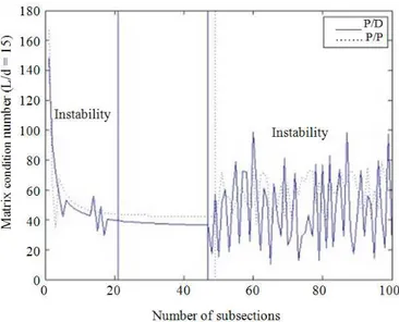
single subsection and the values of the capacitance of the charged conducting cylinder. Interested in assigning subdivisions leading to conditions of stability of the solutions respect the disturbance of the entry results, the choice of the number of N subsections has been derived from the comparison between the two criteria. The first, for each value of the length/diameter ratio, assesses the minimums of the trends of the conditioning numbers K(A) = ||A|| ||A-1||≥1 (graded index of sensitiveness of the solution to the disturbance of the entry data with values as close to the unit as less sensitive it is the system to the disturbance), N increasing for each A matrix drawn per P/D and P/P functions. In certain cases under examination, the drawn trends, even presenting instability for little values of N,settle themselves step by step N increases of value, to produce, then, strong conditions of instability over a certain N given value. By way of example, Fig. 1 shows the trend of the matrix condition number according to the number of subsections for each couple of B/T functions as to the value 15, while Fig. 2 shows the trend of the capacitance per unit of length according to the number of subsections for each B/T couple as to the value 6 of the length/diameter ratio (no restarting for GMRES). In particular, to the i-th minimum, mini (K(A)), it
corresponds an i-th value of N, Ni, so that the first
criterion gives Nthe minimum value of the Ni, min(Ni).
The second criterion assesses the trends of the capacitance (pF) when increasing the number of subsections for each B/T couple and for each resolutive procedure of the linear system until the capacitance values are not affected by evident oscillations due to numerical instability. Labelling Nj the values for N over which, at any case, it occurs a
numerical instability, the second criterion gives N the minimum value of the Nj, min (Nj). So, the final
assignation for N will be Equation (24):
i j
N=min (min(N ), min(N )) (24)
Keeping us, this way in a safety advantage because really far from conditions of instability, but always sufficiently close to the conditions of minimum for K(A). In the case under examination, according to the (24), the final N is tested around 45 units. The comparison for capacitance of specimen (pF), obtained with different B/T functions and for increasing values of length/diameter ratio, have been compared with the analytical solution (Alad and Chakrabarty, 2013) and are reported in Table 1 for each procedure of resolution of the linear system.
Fig. 1. K(A) versus the number of subsections for each couple of B/T functions as to the value 15 of the length/diameter ratio
Fig. 2. C (pF/m) according to the number of subsections
Table 1. Comparison between capacitance values (pF/m) obtained through analytical integration with GMRES, CGS, BicGStab and Gauss-Jordan inversion when varying the length/diameter ratio and for different B/T couples
Gauss-Jordan GMRES CGS BicGStab
Analitical --- --- --- --- L/d Method P/D P/P P/D P/P P/D P/P P/D P/P 6 22.33 25.84 23.44 24.11 23.19 25.12 23.40 25.87 23.12 10 18.55 21.07 21.99 20.91 21.77 20.81 21.23 20.11 22.20 15 16.35 18.35 20.33 18.22 19.96 18.06 20.70 18.37 20.14 20 15.08 16.80 17.14 17.09 17.00 16.20 17.10 16.22 17.14 25 14.22 15.76 16.30 15.76 16.43 15.34 16.43 15.33 16.55 30 13.59 15.01 15.67 14.88 15.80 14.15 15.85 15.07 15.89 60 11.62 12.70 13.64 12.94 13.99 12.30 13.77 12.34 13.15
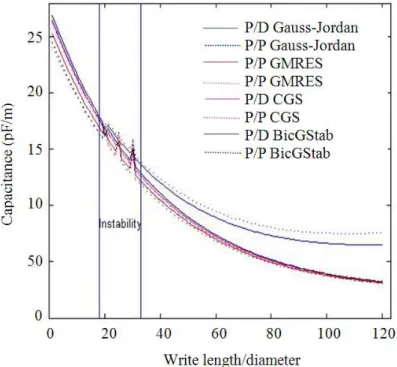
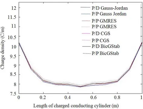
They have been traced, as marked in Fig. 3, the trends of the capacitance (pF/m) according to the length/diameter ratio for each B/T couple and resolutive procedure of the linear system (no restarting for GMRES), highlighting the instability area, too. The distribution of electrostatic charge (C/m) with value equal to 400 of length/diameter ratio for each B/T couple and relatively to each resolutive procedure of the linear system (no restarting for GMRES) is visualized in Fig. 4. In order to evaluate the convergence of the numerical data on the capacitance,
Fig. 5 shows the trend of the capacitance (pF/m) with
value equal to 400 of length/diameter ratio, for each B/T couple and as to each resolutive procedure of the linear system (no restarting for GMRES). To assess the convergence speed of the iterative procedures and considering that when they increase the number of the elements different from zero present in the matrix, BicGStab should be quicker than GMRES, the methods have been tested on A matrixes with number of not null elements, increasing step by step and evaluating the number of iterations required and the CPU-Time. Specifically, with reference to the GMRES procedure, when it increases the length/diameter ratio and for different B/T functions, they have been drawn the dimensions of theA matrix
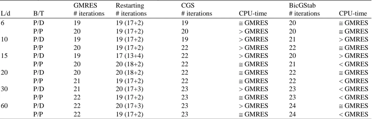
which guarantees the convergence and the correspondent number of iterations in absence/presence of restarting (for GMRES). In this last case, the number of iterations has been differentiated in internal/external iterations, correspondent to the cycles nesting. Finally, as to the CGS and BicGStab procedures, always for different B/T functions and for increasing length/diameter ratio, they have been drawn the dimensions of the A matrix guaranteeing the convergence and the correspondent number of iterations and the comparison too of the CPU-time respect the GMRES procedure. The results are presented in Table 2.
5. CONCLUSION
In the present work, upon the double research about the number of useful subsections and the instability areas got from the comparison between the two criteria of which in the previous paragraph (Fig. 1 and 2), it has been presented a comparative study about P/D and P/P functions used in MoM in terms of complexity, convergence and conditioning of the matrix for the evaluation of C and q in a cylindrical conductor of finite length. The numerical data are presented for each B/T couple in terms of number of conditioning and convergence.
Fig. 3. Capacitance trend (pF/m) according to the length/diameter ratio for each B/T couple and resolutive procedure of the linear system (no restarting for GMRES). The vertical lines single out the area of instability
Fig. 4. Distribution of electrostatic charge (C/m) with value equal to 400 of length/diameter ratio for each B/T couple and as to each resolutive procedure of the linear system (no restarting for GMRES)
Fig. 5. Capacitance trend (pF/m) with value equal to 400 of length/diameter ratio for each B/T couple and as to each resolutive procedure of the linear system (no restarting for GMRES)
Table 2. Comparison between GMRES (without and with restarting), CGS and BicGStab in terms of dimension of the matrix guaranteeing the convergence, number of iterations (differentiated into internal and external) and CPU-time according to length/diameter ratio and for different B/T couples
GMRES Restarting CGS BicGStab
L/d B/T # iterations # iterations # iterations CPU-time # iterations CPU-time
6 P/D 19 19 (17+2) 19 ≅ GMRES 20 ≅ GMRES P/P 20 19 (17+2) 20 > GMRES 20 ≅ GMRES 10 P/D 19 19 (17+2) 19 > GMRES 21 > GMRES P/P 20 19 (17+2) 22 > GMRES 22 ≅ GMRES 15 P/D 19 17 (13+4) 22 > GMRES 20 > GMRES P/P 20 20 (18+2) 22 ≅ GMRES 21 < GMRES 20 P/D 20 20 (18+2) 22 ≅ GMRES 22 ≅ GMRES P/P 21 19 (17+2) 22 ≅ GMRES 22 < GMRES 30 P/D 21 20 (17+3) 23 > GMRES 23 < GMRES P/P 22 19 (17+2) 23 ≅ GMRES 23 < GMRES 60 P/D 22 20 (17+3) 23 > GMRES 24 ≅ GMRES P/P 22 19 (17+2) 23 ≅ GMRES 24 < GMRES
Moreover, they have been compared three leading iterative methods for solving the respective linear systems in Krylov’s subspaces (GMRES, CGS and BicGStab) on matrixes with a number of elements different from zero increasing step by step, evaluating times of execution and number of necessary iterations. From the analysis of Table 1 it can be noticed the good adherence of the results obtained as to the analytical solution (Alad and Chakrabarty, 2013), the capacitance values (pF/m) obtained with GMRES (no restarting), CGS, BicGStab and with Gausse-Jordan’s inversion when varying the length/diameter ratio and for P/P couples. Variation of capacitances of hollow cylinder with height by diameter ratio using P/D and P/P methods and analytical one have been carried out by means Gauss-Jordan, GMRES. CGS and BicGStab algorithms. In particular, as for all the procedures of resolution considered, P/P with BicGStab performs better the analytical results (Fig. 3). The charge distribution q (Fig.
4) presents maximums at the extremity of the specimen
and, through marked inclinations, it is ranged the minimum in correspondence at the middle of the specimen. The convergence data show that BicGStab procedure with P/P couple that converges faster than other procedures (Fig. 5) presenting a better adherence to the analytical solution. The comparison between GMRES (with and without restarting), CGS and BicGStab in terms of matrix dimensions guaranteeing the convergence, the number of iterations (differentiated into internal and external) and CPU-time according to the length/diameter ratio and for different B/T couples, presented in Table 2, has highlighted that P/P BicGStab, even presenting an increase of the number of iterations, provides a decreasing trend of CPU-time. Obviously,
what has been dealing with in the present work is desirable to be tested on specimen with more complex geometries and on more matrixes comparing BicGStab with GMRES with different restarting options of adaptive type. However, the choice of operating on a cylindrical specimen was dictated by the fact that more complex specimens can be treated modularly as a set of cylindrical elements. Obviously, the present study has the limitation of treating only two pairs of functions B/T. In the future, it would required a more detailed study of comparison between functions belonging to a set of pairs B/T characterizing by a bigger cardinality. Because of the bad conditioning of the matrix of the system, it is imperative the exploitation of suitable pre-conditioners.
6. REFERENCES
Alad, R.H. and S.B. Chakrabarty, 2013. Capacitance and surface charge distribution computations for a satellite modeled as a rectangular cuboid and two plates. J. Electrostat., 71: 1005-1010. DOI: 10.1016/j.elstat.2013.09.006
Alad, R.H. and S.B. Chakrabarty, 2012. Inverstigation of different basis and testing functions in method of moments for electrostatic problems. Prog. Electromagnet. Res. B, 44: 31-52.
Angiulli, G. and M. Versaci, 2002. A neuro-fuzzy network for the design of circular and triangular equilateral microstrip antennas. Int. J. Infrared Millimeter Waves, 23: 1513-1520. DOI: 10.1023/A:1020333704205 Angiulli, G. and M. Versaci, 2003. Resonant frequency
evaluation of microstrip antennas using a neural fuzzy approach. IEEE Trans. Magnet., 39: 1333-1336. DOI: 10.1109/TMAG.2003.810172
Apaydin, G. and L. Sevgi, 2012. Method of Moments (MoM) modeling for resonating structures: Propagation inside a parallel plate waveguide. Applied Computat. Electromagn. Soc. J., 27: 842-849.
Chakrabarty, S.B., 2002. Capacitance of dielectric coated cylinder of finite axial length and truncated cone isolated in free space. IEEE Trans. Electromagn.
Compatib., 44: 394-398. DOI:
10.1109/TEMC.2002.1003406
Elangovan, G. and J.R. Perinbam, 2012. Wideband E-Shaped microstrip antenna wireless sensor networks Am. J. Applied Sci., 9: 89-92. DOI: 10.3844/ajassp.2012.89.92
Kumar, P.R. and R.M.S. Parvathi, 2012. Multiple input multiple output system with space time block coding and orthogonal frequency division multiplexing. J.
Comput. Sci., 8: 449-453. DOI:
10.3844/jcssp.2012.449.453
Liu, J., 2011. A comparative study of block preconditioners for incompressible flow problems. J.
Math. Stat., 7: 255-261. DOI:
10.3844/jmssp.2011.255.261
Misran, N., M.T. Islam and N.K. Jiunn, 2008. Design and development of broadband inverted e-shaped patch microstrip array antenna for 3G wireless network. Am. J. Applied Sci., 5: 427-434. DOI: 10.3844/ajassp.2008.427.434
Mouheddin, S. and B.H.T. Jamel, 2009. Indoor characterisation using high-resolution signal processing based on five-port techniques for signal input multiple output systems. Am. J. Eng. Applied Sci., 2: 365-371. DOI: 10.3844/ajeassp.2009.365.371
Prarthan, D.M. and S.B. Chakrabarty, 2001. Capacitance of dielectric coated metallic bodies isolated in free space. Electromagnetics, 31: 294-314.
Sadiku, M.N.O., 2000. Numerical Techniques in Electromagnetics. 2nd Edn., CRC Press, ISBN-10: 1420058274, pp: 760.
Sadiku, M.N.O., 2010. Elements of Electromagnetics. 5th Edn., Oxford University Press, New York, ISBN-10: 0195387759, pp: 845.
Sultan, K.M., H.H. Abdullah and E.A. Abdallah, 2012. Method of moments analysis for antenna arrays with optimum memory and time consumption. Proceedings of the Progress in Electromagnetics Research Symposium, Mar. 27-30, Malaysia, pp: 1353-1356.
Wu, J., S.K. Khamas and G.G. Cook, 2012. Moment method analysis of a conformal curl antenna printed within layared dielectric cylindrical data. IEEE Trans. Antennas Propagat., 61: 3912-3917. DOI: 10.1109/TAP.2013.2254440
Zhang, K., J. Ouyang, F. Yang, C. Wu and Y. Li et al., 2013. Radiation analysis of large antenna array by using periodic equivalence principle algorithm. Progress Electromagn. Res., 136: 43-49. DOI: 10.2528/PIER12110507