DISCUSSION PAPER SERIES
IZA DP No. 11625
Davide Azzolini
Alberto Martini
Enrico Rettore
Barbara Romano
Antonio Schizzerotto
Loris Vergolini
Testing a Social Innovation in Financial
Aid for Low-Income Students:
Experimental Evidence from Italy
Any opinions expressed in this paper are those of the author(s) and not those of IZA. Research published in this series may include views on policy, but IZA takes no institutional policy positions. The IZA research network is committed to the IZA Guiding Principles of Research Integrity.
The IZA Institute of Labor Economics is an independent economic research institute that conducts research in labor economics and offers evidence-based policy advice on labor market issues. Supported by the Deutsche Post Foundation, IZA runs the world’s largest network of economists, whose research aims to provide answers to the global labor market challenges of our time. Our key objective is to build bridges between academic research, policymakers and society.
IZA Discussion Papers often represent preliminary work and are circulated to encourage discussion. Citation of such a paper should account for its provisional character. A revised version may be available directly from the author.
Schaumburg-Lippe-Straße 5–9
53113 Bonn, Germany Email: [email protected]: +49-228-3894-0 www.iza.org
IZA – Institute of Labor Economics
DISCUSSION PAPER SERIES
IZA DP No. 11625
Testing a Social Innovation in Financial
Aid for Low-Income Students:
Experimental Evidence from Italy
JUNE 2018
Davide Azzolini
FBK-IRVAPPAlberto Martini
Università del Piemonte Orientale and ASVAPP
Enrico Rettore
University of Trento, FBK-IRVAPP and IZA
Barbara Romano
ASVAPPAntonio Schizzerotto
University of Trento and FBKLoris Vergolini
ABSTRACT
IZA DP No. 11625
JUNE 2018
Testing a Social Innovation in Financial
Aid for Low-Income Students:
Experimental Evidence from Italy
1This paper presents the results of a randomized controlled trial aimed at testing the effectiveness of an innovative intervention of asset building (Percorsi) on high school students’ transition to the university. Contrary to most traditional forms of financial aid, the tested intervention is expected to enhance an active involvement of the families and imposes a strong conditionality in the use of the benefits. The experiment, called ACHAB (Affording College with the Help of Asset Building) has been carried out in the province of Torino (Northwest Italy) between 2014 and 2017. For the evaluation purpose, an ad hoc survey has been carried out to collect longitudinal information on enrolment decisions and academic performances (number of exams and persistence) during the first semester and at the beginning of the second year. External data and applicant baseline information were used to perform a multidimensional targeting strategy aimed at identifying the ‘target population’, i.e. those students who were at risk of giving up their university enrolment decisions because of economic reasons. The experimental results point to the existence of positive and significant effects of the program on university enrolment and sizeable and significant positive effects on academic performance and university persistence. The effects of the program are significantly larger for students coming from vocational schools than for students who completed technical or general secondary schools.
JEL Classification: C90, D04, I22, I24
Keywords: higher education, social inequality, financial aid, asset building, randomized controlled trial
Corresponding author:
Enrico Rettore
Department of Sociology and Social Research University of Trento
Via Verdi 26 38122 Trento Italy
E-mail: [email protected]
1 The authors are especially greateful to Silvia Cordero, William Revello, Erich Battistin and Ugo Trivellato for suggestions and comments; to Giovanni Minchio, Simone Schüller and Elena Vettoretto for outstanding contribution to the research; to Laura Mclean for her excellent translations and to the participants at workshops at the various institutions we visited. The authors acknowledge the financial support of the European Union through Grant Agreement VS/2014/0571.
1 Introduction
Although University attendance has risen substantially over the past half century, this gain has been unevenly distributed. There is evidence of low-income families being unable to afford a university education for their children. Contrary to the ideal of higher education qualifications achieved solely because of one’s own intellectual capacity, learning ability, and former school performance, several recent comparative analyses show that family socioeconomic background still strongly affects the chances of enrolling at university and getting a tertiary qualification (Shavit et al. 2007; Bernardi & Ballarino 2016). As education is an important intergenerational and career mobility resource, social inequality in educational opportunities generates longlasting disparities in individuals’ lives.
Different forms of financial aid, from scholarships to loans, have been tried to reduce inequality of access to university education. The purpose of ACHAB (Affording College with the Help of Asset Building) is to provide an experimental test of the effectiveness of a promising but largely untested policy instrument: an asset building program aimed at facilitating access to post-secondary education among high school students from low income families. To enter and stay in the program (Percorsi), families are required to regularly save small amounts of money while their children are in high school. The strong incentive is that each euro saved is supplemented by four euro from a private donor. The conditionality is that the resulting balance is spent for documented university-related expenses.
2 Literature review
2.1 Financial aid policy
Policy-makers have three broad options to make university education more affordable. The first option is providing direct financial aid, in the form of scholarships, grants or tuition waivers conditional on economic need and/or on satisfactory academic performance. The second option is providing some form of collateral to students to enable them to borrow against future earnings by offering low-interest student loans. Third, policy makers can subsidize (public) universities, so that tuition paid by the families covers only a small fraction of the costs and university becomes automatically affordable for the great majority of families. Objections to almost-free university education include being fiscally regressive, and breeding mediocrity, because higher ability/income students tend to stay away from public universities, when there exist a private - and expensive - alternatives on offer.
Countries use different combinations of these options. The United States are a useful example because they deploy a full mix of solutions which allows them to accumulate evidence of the effectiveness of the alternatives. The most widespread form of financial aid here as in other countries is based on the supply of monetary incentives such as grants and scholarships that can be awarded according to merit and/or financial need. Previous studies, mostly based on the US experience, show positive effects of these measures on both enrolment rates (Dynarski 2002, 2003; Angrist et al. 2016) and subsequent academic performance—such as completion and drop-out rates, average grades and
2
and Dynarski (2012) critically examine the evidence on the cost-effectiveness of different forms of student aid and conclude that “simple and transparent programs appear to be most effective” and that “programs that link money to incentives […] appear to be particularly effective”. A widely quoted estimate puts the effect of $1,000 of financial aid (or reduction in college costs) as generating 3-4 percentage point increase in the college enrolment rate among students from low-income families (Castleman and Long, 2012).
In Europe, where the (tuition) costs of attending university are generally lower, the results of financial aid are more mixed. While in France, Sweden and Denmark there are positive effects (Fack and Grenet 2015; Fredriksson 1997; Nielsen et al. 2010, respectively), in Germany there is no general accordance about the effectiveness of financial aid on enrolment (Baumgartner and Steiner 2006; Stenier and Wrohlich 2012). The results are puzzling also for academic performance: Leuven at al. (2010) did not find any effect for the case of the University of Amsterdam, while Belot et al. (2007), focusing on the Neatherlands, showed that a reduction in the grant duration had small positive effects on average grades.
Tuition fees are found to be a relevant determinant of enrolment choices (Long 2004). Hence, policy measures intended to reduce or eliminate (Domina 2014) them generally exert positive effect on enrolment decisions. Also in line with these studies, Hübner (2012) found that the introduction of tuition fees in some German states reduced dramatically university enrolment.
The most critical financial aid is perhaps the one based on student loans. This way of financing education has increased rapidly in recent decades and brought along concerns about the consequences
of the loans for the new generations of young adults (Goldrick‐Rab et al. 2014). Moreover, existing
evidence suggests that they are not effective in fostering university participation and persistence (Dowd and Coury 2006; Malcom and Dowd 2012). Marx and Turner (2017) found no effect of loan offers on enrolment but reported an increase in the average grade as well as in the number of credits achieved. Neill (2008) found a positive effect of loans on university enrolment in Canada, but this result is limited to the subgroup of students living outside their parents’ house.
2.2 Asset-building programs
The above-described financial aid solutions have different drawbacks and the right mix remains a contentious issue in most countries. Particularly, all the reviewed approaches have two common traits: they do not impose any conditionality on the use of the funds received as loan or scholarship, and they do not involve the families into an active role.
The latter represent a non-negligible limitation: as emerging from a well-established strand of literature, children of socioeconomically deprived families struggle to obtain high educational degrees because of a mix of financial constraints and low educational expectations of their parents (Goldrick-Rab et al. 2016). Financial aid policy that successfully manages to attenuate disadvantaged families’ financial constraints as well as enhance their educational expectations looks like a promising solution to effectively tackle social inequality in education attainment (Kim et al. 2018).
3
Individual development accounts based on asset-building mechanisms are increasingly seen as a viable policy option to foster families’ long-term development goals (Sherraden 1991, Beverly et al. 2013). Asset building provides a mechanism for low-income families to start saving regularly small amounts of money. The savings are then heavily topped-up by a donor but are also constrained to be used to pay for education related expenses. As a tool for fighting poverty, asset building has steadily spread since the pioneering experiences of the early 1990s (OECD, 2003). For example, in the UK, each pound deposited into a so-called “Saving Gateway account” is matched by the UK government at a certain rate and up to a monthly contribution limit. Matching provides a transparent and understandable incentive for eligible individuals to place funds in an account. These matched incentive programs are aimed at encouraging either a general or a specific saving habit. In some instances, savings are incentivized for a specific goal (home ownership, self-employment, small business start-up).
Financial aid based on asset-budilding mechanism has two main comparative advantages over the most classical forms of financial aid such as scholarships, loans or tuition waivers (Dynarski and Scott-Clayton 2013). First, by stimulating stronger and longer-lasting family commitment and financial plans, asset-building programs trigger parents’ expectations and children’s attitudes toward education by making the entire family more confident about the actual sustainability of long-term education plans (Beverly et al. 2013). Second, typically these programs impose a strong conditionality in the usage of the monetary benefits, thus reducing the risk of stimulating opportunistic behaviors. Moreover, in contexts such as the US, asset-building programs have also been recognized as a potential strategy to reduce students’ reliance on loans (Assets and Education Initiative 2013).
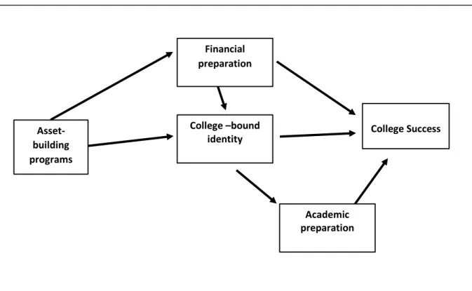
The channels through which asset-building programs can enhance college participation and success are sketched in Figure 1. The direct channel (“financial preparation”) comprises aspects connected to liquidity constraints and the ability of planning the use of disposable economic resources. The indirect channel, instead, operates on both family and students’ college expectations (“the college-bound identity”). The formation of the so-called “college-college-bound identity” could translate into higher college participation both directly and indirectly, by positively affecting academic preparation (i.e., high school results).
Asset-building programs for post-secondary education investments have been implemented in several countries (Loke and Sherraden 2009, Beverly et al. 2013). Nonetheless, evidence about their effectiveness is scarce (Leckie et al. 2010; Cheatham and Elliot 2013; Grinstein-Weiss et al. 2013; Bogle et al, 2016; Mills et al 2016; Kim et al. 2018). The few existing evaluation studies concern multi-purpose indivudal development conducted in Anglo-Saxon countries. They showed relevant impacts on outcomes such as financial literacy and saving behaviour (Russel et al. 2008; Leckie et al. 2010; Elliot and Sherraden 2013; Mills et al 2016). Moreover, they show some evidence of positive effects on post-secondary education enrolment rates (Leckie et al. 2010; Cheatham and Elliot 2013; Grinstein-Weiss et al. 2013).
4
Figure 1: Pathways from asset-building programs to college success
Source: Beverly et al. 2013, p. 4.
Among the individual development accounts that are closer to Percorsi both because they focus only on education investments and because they imply a “rapidly incentivized” savings mechanisms, two - implemented in the United States - are worth being mentioned.
First, the Viking “Advantage” program is an Individual Development Account sponsored by a non-profit organization called Beyond Housing, operating in the Saint Louis area, and set up as a custodial account at Truman Bank. Viking Advantage IDA is a matched-savings account: every dollar saved up to $1,500 is matched with two dollars. IDA savings can be used for application fees, books, tuition, and/or computer purchase at any accredited institution. Eligibility for the program is based on total household income. Student participants must attend one club meeting per month for financial education.
Another example of a program in this vein is offered by the three public universities of Arizona (i.e., Arizona State University, Northwest Arizona University and University of Arizona). The program, called “Earn to Learn”, asks students to earn up to $500 per year of each of the four years of college. This amount is then multiplied by a 8:1 matching multiplier. Hence, each year students can earn $4,000 to pay for tuition, books and other university-related expenses. The matching scholarship is renewable for up to four years depending ongoing funding as long students remain eligible and continue to earn and save $500 each year. Additionally, the program offers coaching for students which includes personal finance training, college readiness training, and ongoing support from the very first day of attending college all the way through graduation.
Asset-building programs Financial preparation College Success College –bound identity Academic preparation
5 2.3 The Italian context
Upper secondary education in Italy is divided into three main tracks: the academic (licei), the technical (istituto tecnico), and the vocational (istituto professionale). These tracks last five years and end with a final state exam (Esame di maturità). All students passing this exam can enrol at the university, independently from the track attended.
Tertiary education is based on a sequential system, which comprises a 3-year Bachelor’s (laurea
breve) and a 2-year specialization (laurea magistrale) degrees, with the latter granting the access to
doctoral programs. Italian public universities’ tuition fees are a small fraction of those charged in other countries (e.g., the US), with tuition averaging €1.000 euro a year. Yet, such low tuition combined with other costs (such as books, transportation, rent, software and Internet access), leaving aside foregone earnings, concur to an average annual cost between €2.500 and €3.000, which might not be affordable by families in severe financial distress (Barone et al. 2014).
In Italy, the main program for funding university participation is the so-called Diritto allo studio (‘Right to study’) that is regulated at the national level and co-financed by the regional governments. It is designed to cover direct costs, and students can have access to it according to family income and academic performance. In addition to this national-regional scheme, there are few small programs funded by local governments or by private foundations that offer further monetary aid. But such interventions are not systematic and are rather scattered throughout the country.
3 Program and experimental protocol
2.1 The program’s main features
Percorsi is a small asset-building program implemented since 2010 by the Ufficio Pio of the Compagnia di San Paolo, a foundation based in Torino, northwest of Italy. The very first aim of Percorsi was to
help families hit by the economic crisis and then forced to give up their children’s education plans. Under this program, eligible families are admitted, and a dedicated savings account opened in their name. To stay in the program, families have to deposit between €5 and €50 a month, for up to six years. Families can deposit up to €2,000 and the savings are supplemented with a 4:1 matching multiplier by the Ufficio Pio. Thus, the maximum of €2,000 saved by the family, supplemented by a maximum grant of €8,000, together make €10,000 available to pay for college, a sum that is in line with the average costs of getting a standard 3-year Italian degree. If spent during high school, the money saved carries a multiplier of 2:1, while the multiplier is 4:1 if the expenses are related to college. As it happens in most asset-building programs, in addition to the savings account, students and their families have to attend a financial education course to remain in the program.
2.2 Recruitment and targeting
The ACHAB demonstration was targeted to all students living in the province of Torino and enrolled in
6
years. In the fall of 2014 and 2015, all high schools in the province of Torino were invested by a promotional campaign, led by Ufficio Pio with the help of a marketing company, with the explicit aim of convincing eligible student to sign up for the program, by filling the on-line application form. The campaign was very effective and led to recruit 1,033 fourth and fifth-year students in the first cohort and 307 fifth-year students in the second.
After student recruiting, the second step concerned the identification, among applicant students, of those who were truly at risk of not being able to continue their education, because of economic hardships. This was achieved by implementing a multidimensional targeting strategy. First, an eligibility criterion based on family income was made explicit to all students: eligible students had to come from families with an ISEE (the national index of the equivalent economic situation of the family) below 25.000 euro. Second, the information provided by applicants in the application form was used to screen out students with too high or too low probability of enrolling at the university, as it will be explained below.
The two sets of students (i.e., ACHAB applicants and students at risk) do not naturally overlap. Students at risk might fail to apply, for many reasons, such as lack of knowledge or lack of trust; while on the opposite side, being the income threshold a very imperfect measure of actual ability to pay, we could have some students not truly at risk still buying what they consider a lottery ticket. The results of the lottery will not change their decisions, although some pure income effect cannot be ruled out. We cannot double guess their true intentions, but we can screen them differently. In what follows, we describe the targeting procedure implemented for the first call’s applicants (school year 2014-2015). The procedure was replicated identically in the second call (school year 2015-2016).
From 1,033 to 945: Eliminating missing data
Of the 1,033 completed applications, some had missing data for some variables such as parental occupation and education and immigration background, that were crucial to predict the likelihood of university enrollment. More precisely, 80 had missing information on some items that result as strong predictors of university enrolment; 8 cases are excluded because they were born before 1991. Such first screening left us with 945 usable cases, still a far cry from the 500 target. Such excess demand offered a chance of experimenting with a multidimensional targeting strategy (Azevedo and Robles 2013), to which we now turn.
Imagine applicants ordered in terms of their predicted probability of going to university, and that probability varies continuously from zero to one. At the two extremes of the probability spectrum, we would expect to find two polarly opposite groups—that we call “never-enrollees”, those with a probability of enrolling almost zero, and “always-enrollees”, those with a probability of enrolling close to one.
7
Given the demonstration set-up, the identification of never-enrollees is based on the answers to specific questions about enrolment intentions included in the application form of the project. Our a priori expectation was that of intercepting relatively few never-enrollees. To be sure, the great majority of students who would not consider enrolling in university did not even apply to ACHAB. However, a special provision is that Percorsi allowed two separate matching multipliers: in addition to the 4:1 multiplier for university-related expenditure, a lower multiplier of 2:1 is allowed for school related expenditure while in high school. So the presence of applicants with no explicit intention to enroll in University but still interested in the program cannot be ruled out. Forty-four students, about 5% of the total applicants, are excluded using the answers they gave to two questions in the application form (Table 1). More precisely, the students who answered “3” to question 3.21 or to question 3.26 are dropped from the analysis. This drop brought the usable population down from 945 to 901.
Table 1 Questions Used To Screen Out Never Enrollees
3.21 Do you think you will enroll at the university right after your diploma?
1. Yes
2. I would like to, but I am afraid that my family cannot afford it 3. No
4. I haven’t decided yet
3.26 If your answer to 3.21 is “I haven’t decided yet”?
1. It is due to my family’s economic situation
2. I am undecided because I am afraid that the university is too difficult for me 3. I am undecided because I am not sure that going to university is worth much
From 901 to 500: minimizing always-enrollees
The next move is aimed at identifying – among the ACHAB applicants – those students that, given their characteristics, look likely they would enroll at the University no matter their assignment to the treatment or the control group. This problem is widely known in the literature as the problem of targeting benefits of social programs. A proper targeting is crucial for the success of ACHAB as well. We needed a way of simulating applicants’ probability of enrolling in university after the completion of high school. To produce these simulations, i.e., to calculate the enrollment probability of each individual, a unique resource from the Province of Trento (Northeast Italy) – the Indagine sui diplomati trentini (Survey on
High School Graduates carried out in the Province of Trento, SHSG henceforth2 – was used.
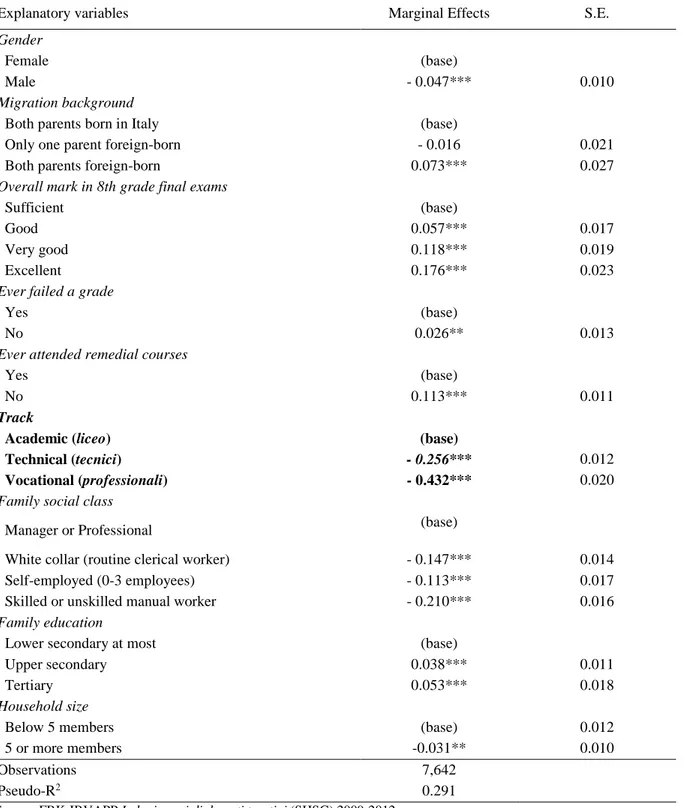
Determinants of the probability of enrollment in university are analyzed by the means of a logistic regression model, whose estimates are shown in Table 2. Confirming existing evidence, the main determinants of University enrolment probability are the type of school attended and family
2 We chose these data over alternative options (such as the Bank of Italy’s Survey of Household Income and
Wealth - SHIW) for two important reasons. First, the SHSG data provide richer and more detailed information on several key aspects, including (a) enrolment intentions and actual enrolment; (b) socio-demographic characteristics; (c) social origins (parental education and parental social class); (d) school career (school type attended, mark obtained on the 8th grade final exam; failure experience; and attendance of remedial courses). Second, the SHSG data cover four high school graduates cohorts, while SHIW is a household survey representative of the entire population.
8
background. The coefficients on type of high school turn out to be largest, motivating our decision to use academic tracks as a randomization blocking variable. The coefficients presented in Table 2 are then applied to each ACHAB applicants’ characteristics in order to predict their individual university enrolment probability.
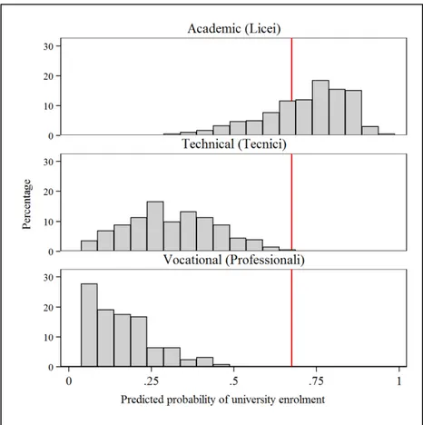
In the meantime, our target was revised to 520, in order to have a small pool of extra cases from which to draw substitutes for the cases of immediate withdrawals from the program. To select the 520 students out of the 901 valid applications, we ranked the ACHAB applicants according to their predicted enrolment probability. Then, we include in the sample 520 students starting from the one with the smallest value of the predicted probability of enrolment. The remaining 381 students (i.e., those with ‘high’ predicted probability of enrolment) are dropped from further use in the analysis. The resulting cut-off in the predicted probability of enrolment is 0.675: only cases with a predicted probability lower than the cut-off point are included in the randomization procedure.
The distribution of the computed predicted probability in the sample of ACHAB applicants is shown in Figure 2. The figure shows that all students who are excluded from the sample come from the academic track. This comes as no surprise considering the size and significance of the coefficients on school type displayed in Table 2.
An identical procedure, one year later
Motivated by the success of the 2014-15 edition, and made aware of the danger of underpowered experiments, the Ufficio Pio decided to increase the sample size by adding another wave of observations to the sample. The applications were not very much in excess. After eliminating these 13 applicants with either missing or invalid information, the number of valid observations amounted to 294. 8 students were dropped as ‘never-enrollees’ and 36 as ‘always-enrollees’. The remaining 250 applicants were admitted to the study and randomized.
9
Table 2 The logistic regression model used to predict the probability of enrollment
Source: FBK-IRVAPP Indagine sui diplomati trentini (SHSG) 2009-2012.
Note: The dependent variable is individual actual enrolment in university. Pooled sample, estimation model additionally contains survey year indicators
* p<.1; ** p<.05; *** p<.01.
Explanatory variables Marginal Effects S.E.
Gender
Female (base)
Male - 0.047*** 0.010
Migration background
Both parents born in Italy (base)
Only one parent foreign-born - 0.016 0.021
Both parents foreign-born 0.073*** 0.027
Overall mark in 8th grade final exams
Sufficient (base)
Good 0.057*** 0.017
Very good 0.118*** 0.019
Excellent 0.176*** 0.023
Ever failed a grade
Yes (base)
No 0.026** 0.013
Ever attended remedial courses
Yes (base)
No 0.113*** 0.011
Track
Academic (liceo) (base)
Technical (tecnici) - 0.256*** 0.012
Vocational (professionali) - 0.432*** 0.020
Family social class
Manager or Professional (base)
White collar (routine clerical worker) - 0.147*** 0.014
Self-employed (0-3 employees) - 0.113*** 0.017
Skilled or unskilled manual worker - 0.210*** 0.016
Family education
Lower secondary at most (base)
Upper secondary 0.038*** 0.011
Tertiary 0.053*** 0.018
Household size
Below 5 members (base) 0.012
5 or more members -0.031** 0.010
Observations 7,642
10
Figure 2 Distribution of predicted university enrolment probability by high school track
Note: First cohort data. The vertical line indicates the cut-off (0.675).
2.3 Randomization
This section illustrates the randomization procedure performed to assign 300 individuals among the 716
eligible applicants3 to the treatment group and the rest to the control group. We formed nine blocks
based on the cohort of entry (4th or 5th year) and on secondary school track (academic, technical or vocational). This way we obtained nine separate randomized experiments (Bloom 2006). The choice of these blocking factors reflects the fact that high school track is the strongest predictor of students’ university enrolment probability. To guarantee that the treated cases have a balanced distribution across bl ocks, we randomized one block at a time to reach block-specific targets. Table 3 shows the sample disposition after randomization.
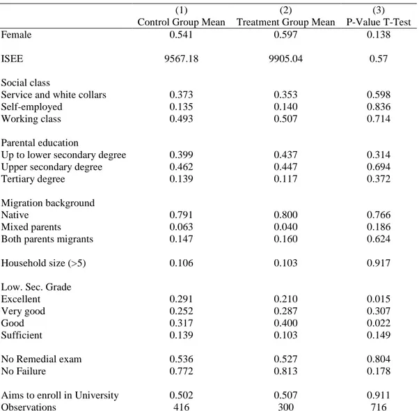
The assessment of statistical equivalence of the assignment to treatment or controls groups is based on the following individual and family characteristics collected in the application form: gender, final mark in the 8th grade, grade retention, participation in remedial courses; predicted university enrolment probability and self-reported enrolment intention; family background (ISEE, social class, parental education, immigrant background) and household size. Table 4 displays the balancing tests for
3
Out of the 770 valid applications, only 716 are actually used because of two reasons. First, 29 applicants (22 in the first
two cohorts and 7 in the third cohort) were replaced due to irregularities in their application forms. Second, 25 students belonging to cohort 2 and assigned to the control group, reiterated their application in the subsequent school year: 14 of them ended up again in the control group and 11 in the treatment group. We consider these reiterated applications as students belonging to cohort 2 and the 11 cases are treated as crossovers.
11
the full sample. The first two columns of Table 4 report the mean values for each of the characteristics, whereas the third column reports the p-values of the t-test of the difference.
Table 3 Disposition of the three coorths of ACHAB applicants
Table 4 Balancing test for the full sample
(1) (2) (3)
Control Group Mean Treatment Group Mean P-Value T-Test
Female 0.541 0.597 0.138
ISEE 9567.18 9905.04 0.57
Social class
Service and white collars 0.373 0.353 0.598
Self-employed 0.135 0.140 0.836
Working class 0.493 0.507 0.714
Parental education
Up to lower secondary degree 0.399 0.437 0.314
Upper secondary degree 0.462 0.447 0.694
Tertiary degree 0.139 0.117 0.372
Migration background
Native 0.791 0.800 0.766
Mixed parents 0.063 0.040 0.186
Both parents migrants 0.147 0.160 0.624
Household size (>5) 0.106 0.103 0.917
Low. Sec. Grade
Excellent 0.291 0.210 0.015 Very good 0.252 0.287 0.307 Good 0.317 0.400 0.022 Sufficient 0.139 0.103 0.149 No Remedial exam 0.536 0.527 0.804 No Failure 0.772 0.813 0.178
Aims to enroll in University 0.502 0.507 0.911
Observations 416 300 716
Notes: F-test of joint significance from a regression of all characteristics on the probability to be assigned to
the treatment group - F-test (15, 700) = 1.09, Prob > F. = 0.358. (Cohort ONE) 13th grade in 2014-2015 (Cohort TWO) 12th grade in 2014-2015 (Cohort THREE) 13th grade in 2015-2016 Applicants 530 503 307 Valid applicants 483 462 294
Screened out applicants 207 218 44
Eligible applicantsa 256 242 218
Treated 103 97 89
12
Tables A.1-A.5 (Appendix A) present balancing tests for cohort and track. For most individual and family characteristics there are no significant differences between treated and controls groups. To control for the small existing imbalances, the impact estimates will be obtained via regression models that allow adjusting the estimates by adding relevant covariates.
4 Data and variables
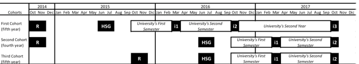
In addition to the baseline information collected with the application form, the outcome data were collected with follow-up interviews conducted via CATI (Computer-Assisted Telephone Interviewing) and carried out by a subcontractor, under the ACHAB team supervision. These surveys took place in Spring and Fall of 2016 and 2017 (Figure 3).
The most relevant dimensions for the outcomes are connected to university enrolment and retention. In other words, we collect information on: i) university enrolment; ii) exams taken at the end of the first semester/first year/second year as proxies of retention; iii) enrolment in the second year as a measure of university persistence. These outcomes are coded as dichotomous variables. University enrolment takes value 1 if the student is enrolled at the university and 0 otherwise. The second outcome is passing at least one exam during the first semester, which is coded as taking value 0 for both those who did not take any exam the first semester and for those who never enrolled and 1 otherwise. The third outcome is passing at least two exams during the first year, which is coded similarly to the previous outcome. The last outcome is the persistence at the university and it takes value 1 if the students is
enrolled at the second year and value 0 for those who drop-out and for those who never enrolled. 4
Figure 3 The ACHAB data collection plan
Legend: R=randomization; HSG=High school graduation; i1=First interview; i2=Second interview; i3=Third interview.
4Enrolment in post-secondary non-tertiary courses is not counted as participation in higher education, as the 4:1 matching
grant provided by Percorsi is strictly limited to University attendendance.
Oct Nov Dec Jan Feb Mar Apr May Jun Jul Aug Sep Oct Nov Dic Jan Feb Mar Apr May Jun Jul Aug Sep Oct Nov Dic Jan Feb Mar Apr May Jun Jul Aug Sep Oct Nov Dic First Cohort (fifth year) i1 i2 i3 Second Cohort (fourth year) i1 i2 Third Cohort (fifth year) i1 i2 Cohorts University's First
Semester University's Second Semester University's Second Year University's First Semester 2017 2014 2015 2016 R R University's First Semester University's Second Semester University's Second Semester R HSG HSG HSG
13 4.1 Attrition
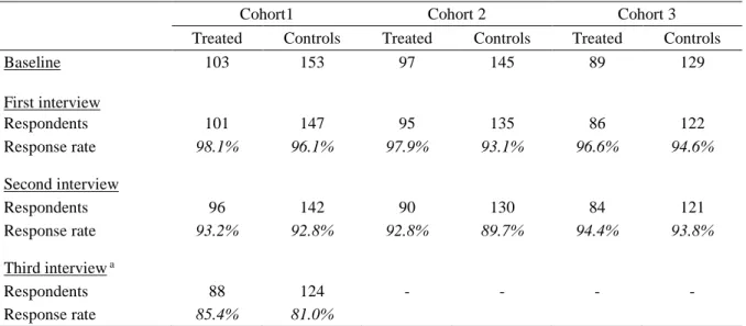
The CATI interviews process went smoothly and produced excellent results, as shown in Table 5. The non-response rates were low and the treated and controls differential attrition was well below the standards set by the What Works Clearinghouse (2014). The comparison conducted in Appendix B shows that the distributions of the characteristics of respondents changes very little overtime as the sample slowly loses some of its members to attrition.
Table 5 Response rates
Cohort1 Cohort 2 Cohort 3
Treated Controls Treated Controls Treated Controls
Baseline 103 153 97 145 89 129 First interview Respondents 101 147 95 135 86 122 Response rate 98.1% 96.1% 97.9% 93.1% 96.6% 94.6% Second interview Respondents 96 142 90 130 84 121 Response rate 93.2% 92.8% 92.8% 89.7% 94.4% 93.8% Third interview a Respondents 88 124 - - - - Response rate 85.4% 81.0%
a The data of the third interview are not analyzed in this paper.
5 The analysis of program impacts
The estimates of program impacts are presented as regression-adjusted differences in means. We run regressions including covariates for three main reasons: i) increasing in the precision of all the estimates, notably of the variables used for blocking; ii) correcting for possible group imbalances; iii) carrying out heterogeneity analysis of the program’s impact.
The impact estimates on the four outcomes are obtained through a set of linear probability models:
𝑌𝑌𝑖𝑖= 𝛽𝛽0+ 𝛽𝛽1∙ 𝑍𝑍𝑖𝑖+ 𝛽𝛽2∙ 𝐵𝐵𝑖𝑖+ 𝛽𝛽3∙ 𝑋𝑋𝑖𝑖+ 𝜀𝜀𝑖𝑖
Where Y is the outcome of interest, Z is the treatment assignment, 𝐵𝐵 are the blocking variables (high
school tracking in three levels – academic, technical and vocational – and the school grade attended when entering the program) and X is a set of relevant characteristics (sex, parents income measured through the ISEE index and the student performance in earlier grades: failure and remedial courses) included in order to increase the precision of our estimates. Because of the negligible non-compliance to treatment assignment (only 11 crossovers and zero no-shows), we present intent-to-treat (ITT) effects.
14 5.1 The homogeneous impact model
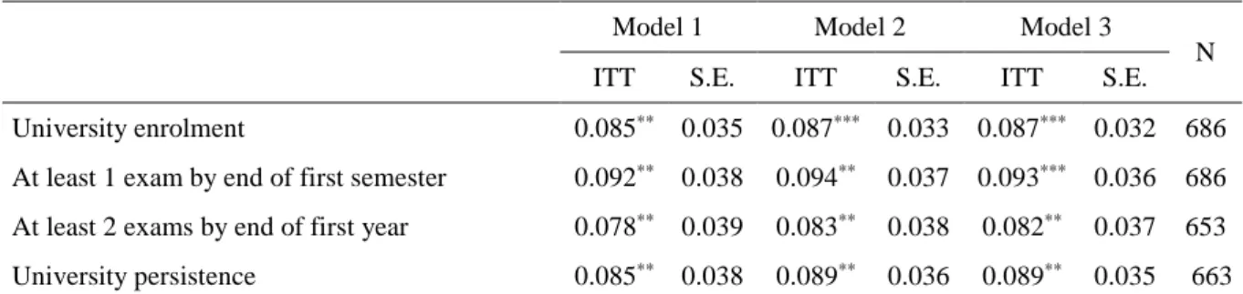
The three models presented in Table 5, going from left to right, contain an increasing number of control variables. More precisely, Model 1 does not contain any controls, Model 2 includes the blocking variables and Model 3 adds some relevant characteristics listed above. Table 6 shows how little the estimated impact varies across models. As expected, the simple inclusion of additional explanatory
variables does not affect significantly the estimated value of β, the coefficient of the treatment status, in
any relevant way. The completed list of all the estimated coefficients are shown in Appendix C. Table 6 shows the coefficients of the random assigment variable Z.
Table 6 Estimates of homogeneus program effect and their robust standard errors
Model 1 Model 2 Model 3
N ITT S.E. ITT S.E. ITT S.E. University enrolment 0.085** 0.035 0.087*** 0.033 0.087*** 0.032 686
At least 1 exam by end of first semester 0.092** 0.038 0.094** 0.037 0.093*** 0.036 686
At least 2 exams by end of first year 0.078** 0.039 0.083** 0.038 0.082** 0.037 653
University persistence 0.085** 0.038 0.089** 0.036 0.089** 0.035 663
Note: Model 1 does not contain any control variables; Model 2 controls for the blocking variables; Model 3 controls for the blocking variables and for sex, ISEE, school career (failure and remedial courses).
* p<.10, ** p<.05, *** p<.01
Note that the precision of the estimated coefficients does increase with the inclusion of more explanatory variables, but to a trivial extent: see for example the coefficients of the variable enrolled in a University from 0,035 (Model 1), to 0,033 (Model 2), and to 0,032 (Model 3).
Looking at the causal effects estimated by Model 3, the impact on the outcome “University enrolment” is about 8.7 percentage points on average, and it is significantly different from zero; almost the same values (about 8.9 percentage points) we get for the outcome “University persistence”. Thus, on average, receiving the ACHAB financial aid offer improves University enrolment by about 9 pp.
The other two outcomes, “at least 1 exam during first semester” and “at least 2 exams during first year, suggests that ACHAB’s impact might be slightly deteriorating over time: the likelihood that an ACHAB student takes one exam in the first semester is slightly above 9 percentage points, while that of taking two during the first year is slightly above 8 percentage points. Yet, the two estimates are not significantly different from one another.
5.2 Impact heterogeneity
A substantial heterogeneity is hiding behind the estimates shown in Table 6. We conduct an heterogeneity analysis with respect to each of the four outcomes and the two blocking variables, namely upper-secondary school track (Table 7) and lenght of exposure to the program (Table 8). The OLS regression are specified as in Model 3 (shown in Table 6).
15
technical track, to an intermediate result (+9pp) for the academic track, to a more substantively and statistically significant +20pp among vocational students. Documenting the existence of such heterogeneity represents the most important finding of this part of the analysis.
Table 7 Heterogeneity of impacts, by high school track
Academic Technical Vocational
ITT S.E. N ITT S.E. N ITT S.E. N
University enrolment 0.091* 0.040 333 0.047 0.059 249 0.205** 0.102 104
At least 1 exam by end of first
semester 0.069 0.049 333 0.046 0.062 249 0.333
*** 0.099 104
At least 2 exams by end of first
year 0.079 0.051 315 -0.003 0.063 238 0.349
*** 0.096 100
University persistence 0.071 0.045 321 0.051 0.063 240 0.274***
0.103 102 The models control for the blocking variables and for sex, ISEE, school career (failure and remedial courses).
* p<.10, ** p<.05, *** p<.01
Let us look at the other outcomes shown on the other outcomes for students from the vocational track. Without ACHAB, the probability of taking at least one exam during the first semester, and that of taking at least two in the first year, would be much lower: partipation in ACHAB makes students from vocational schools progress through the first year in University faster than they would otherwise. These results have important implications for financial aid policy. The evidence gathered here suggests that the available resources should be targeted explicitly to the students from vocational schools. For these students, the program’s cost-effectiveness is highest, not only because the program’s impact is the largest but also because the deadweight (i.e., the share of students that would go at the university even in the absence of the incentive, that is the levels observed among the controls, Table 9) is the smallest (44.1% vs. 77% in the academic track).
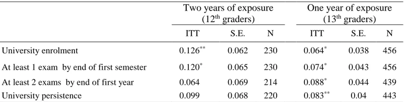
The second key finding is the role played by the length of exposure to the program (1 school
year for 13th graders; 2 school years for 12th graders). As shown in Table 8, students recruited in the 12th
grade show a higher enrolment than the others. Concerning university persistence (i.e., enrolment in
university for the second year), the point estimates indicate that students recruited in the 12th grade have
slightly higher chances of continuing the university studies, yet the estimate is not statistically significant. To shed further light on this point further research and replication studies are needed.
Table 8 Heterogeneity of impacts, by lenght of exposure to the treatment
Two years of exposure (12th graders)
One year of exposure (13th graders)
ITT S.E. N ITT S.E. N
University enrolment 0.126** 0.062 230 0.064* 0.038 456
At least 1 exam by end of first semester 0.120* 0.065 230 0.074* 0.043 456
At least 2 exams by end of first year 0.064 0.069 214 0.088* 0.044 439
University persistence 0.099 0.068 220 0.083** 0.04 443
16
* p<.10, ** p<.05, *** p<.01
Table 9 Average outcome for control units
Overall
Track Graders
Academic Technical Vocational 12th 13th
University enrolment 67.1 77.7 62.2 44.1 53.3 74.0
At least 1 exam by end of first semester 56.4 68.0 52.7 27.1 45.2 62.1 At least 2 exams by end of first year 52.7 64.0 50.7 19.4 40.2 58.9
University persistence 59.3 73.4 51.8 31.0 42.3 67.7
6 More facts about the treated and the treatment
This section provides a description of how the different components of the treatment were implemented during the experimental period. First of all, all students assigned to the treatment actually complied with the assignmnet by actually starting to make deposits (zero noshows). As already remembered above, 11 students assigned to the control group in the first call, reapplied in the second call and got eventually access to the program (we label them as crossovers).
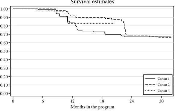
Figure 4 How long did they stay on the program?
A second important piece of information - first of all for program administrators who want to know how to allocate their resources – is students’ retention in the program. Figure 4 shows Kaplan-Meier survival function estimates for the three cohorts. Considering cohorts one and two, 30 months after the access to the program, about 30-34% of students dropped out either because they failed to fulfil the savings requirement or because they abandoned school. It is apparent that the grade attended by students at
0.00 0.10 0.20 0.30 0.40 0.50 0.60 0.70 0.80 0.90 1.00 0 6 12 18 24 30
Months in the program
Cohort 1 Cohort 2 Cohort 3
17
enrolment in the program made a difference for their survival. While for cohort one (13th graders), the
big drop occurs around the end of the first year, for cohort two (12th graders) a similar drop occurs at
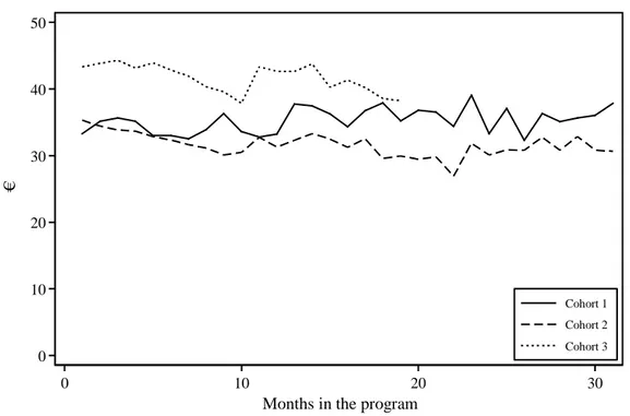
the end of second year. As far as chort three is concerned, the behavior is the similar to that of cohort one in the first months, but then the line is truncated as they entered the program one year later and they are no longer observed. Figure 5 shows the monthly average amounts saved by the ACHAB students and their families. The first two cohorts saved a bit less—between 30 and 40 euro—while the third cohort did save more, about an extra 10 euro a month.
Figure 5 How much did they save?
The program’s rules allowed a wide variety of choices and behaviors. For example, if streched over 6 years, even an average contribution between 25 and 30 a month allows the student to have access to the full contribution of €2,000, that in turns translate into a full matching grant of 8,000 euro. The amount saved has a direct consequence for the likelihood that a family reaches the maximum allowable grant of 2,000 within the horizon of 6 years. At full load, the maximum is reached in 40 months, that is, in slightly more than 3 years. At a lower average of 40 euro per month, it takes 50 month, while at 30 euro a month, reaching 2000 it takes 67 months. Lower savings levels, instead, would result in loss in obtainable matching grants.
On average, in the first 30 months, students of cohort 1 and 2 saved about 790 and 805 euros, respectively. They obtained matching grants of 1768 and 1200, respectively. This reflects not only the amount of money saved but also the use of the matched grant, for either secondary education (x2) or tertirary education (x4) expenditures, with cohort 1 students showing clearly higher transition rates to university. Considering the composition of the expenditures, on the whole sample, tuition fees account for about 34% of all expenses, followed by PC and other digital devices (27%). Transport accounted for 18% and books for 6%. Rent only accounts for less than 5% and is explained by the fact that the great
0 10 20 30 40 50 € 0 10 20 30
Months in the program
Cohort 1 Cohort 2 Cohort 3
18
majority go to one of the local universities, and they keep living with their parents. Future analyses will consider how different groups of students (i.e., defined by their parental socioeconomic background) made use of the program and the extent to which they could benefit from it.
Finally, concerning participation in the financial education classes, ACHAB students participated to a great extent to the classes (only 14% of students were absent for up to 20% of the lessons). Moreover, less than 2 out of ten students had the habit of saving monre for long-term goals (e.g. vacations or paying fees); and 74% of the students agreed that the finantial literacy course made
them change their savings habits.5
Table 10 On what do they spend the money? (Euros)
Expenditure type Cohort 1 Cohort 2 Cohort 3 Total University fees 72,134 33,097 39,319 144,549 PC and other digital devices 42,193 33,306 39,373 114,872 Transport 26,296 23,089 25,911 75,296 Books 16,120 1,726 7,584 25,430 Rent 9,050 3,023 2,103 14,176 Other 16,338 26,436 10,797 53,571 Total 182,131 120,675 125,087 427,893
7 Discussion and conclusions
What we have provided in this report is a picture of a succesful program, one that with minimal administrative costs is able to deliver an innovative and effective form of financial aid to low-income students. Understanding the channels through which Percorsi increased students‘ transition and retention at the University is of utmost importance. Integrating the experimental results presented above
with qualitative data gathered throughout the project,6 three main mechanisms seem to have played a
major role.
Reduced economic barriers. The reduction of economic barriers occurs at two different stages
of the program and thus affects two different outcome variables: in high school, before university enrolment: the guarantee of having a fixed sum of money (determined by the individual’s own savings behaviour) increases university enrolment rates among program participants; after university enrolment: the availability of additional finances frees students from having to work or allows them to work less to support themselves, thus improving their academic performance.
Broadened horizons and enhanced future prospects. Access to financial aid also has a decisive
impact on modifying the recipients' expectations, aspirations and perceptions of self and family. Such
5 This information was collected via a survey of all 300 eligible was fielded to gather more (qualitative)
information on this important topic. The interviews were held through CAWI (computer-aided-web-interviewing): 242 cooperated with the request out of the 300 eligible, with a response rate of 80.1 percent.
6Fifty in-depth interviews with students both treated and controls were conducted. More precisely: 20
pre-randomization interviews; 5 interviews with the Ufficio Pio staff; 21 post-pre-randomization interviews, about one third treated cases, two thirds controls.
19
changes can make a difference not only in whether they decide to embark on a university course or not, but also in what and where they ultimately choose to study, since attending a longer, more challenging degree course would otherwise be impracticable for those who need to hold down a job. Indirect evidence for this positive shift in attitude is the fact that Percorsi-ACHAB has a greater effect on students who join the program in their fourth year of high school rather than later on, which gives them more time to make sense of their changing perspectives and to implement more ambitious choices.
Encouragement effect. Students admitted to the Percorsi-ACHAB program do not fit the
conventional mould of a scholarship recipient. None of them ranks at the top of their class academically and none come from high schools with a high rate of transition to university. Nonetheless, over the course of extensive interviews and interactions with privileged witnesses, these students reveal that being admitted into the program made them feel as though they had been given a second chance or that it was their first taste of success in a school career marked by a lack of encouragement and a history of bad decisions. This sense of achievement then acts as a springboard for further success, providing an important source of motivation for them to go on to university and complete their required exams.
To conclude, an important result to be stressed is that the program made a difference mainly for the students enrolled in vocational schools. The empirical result also suggest that the overall university performance of vocational students improves when they receive an asset building type of assistance, making them more likely to graduate. The voluntary nature of the program does not allow mechanical generalizations. Yet, it is undisputable that the EU objective of 40 % of the workforce between 25 and 34 year olds holding a tertiary degree will never be achieved in Italy without the contribution from a sizable fraction of those who attended a vocational school.
20
References
Angrist, J., Autor, D., Hudson, S., and Pallais, A. (2016). Updated Results from a Randomized Evaluation of Post-Secondary Aid, Columbia University, Working paper.
Assets and Education Initiative (2013). Building Expectations, Delivering Results: Asset-Based Financial Aid and the Future of Higher Education. In W. Elliott (Ed.), Biannual report on the assets
and education field. Lawrence, KS: Assets and Education Initiative (AEDI).
Azevedo V., and Robles, M. (2013). Multidimensional targeting: Identifying beneficiaries of conditional cash transfer programs, Social Indicators Research, 112(2), 447-475.
Barone, C., Abbiati, G. M., and Azzolini, D. (2014). Quanto conviene studiare? Le credenze degli studenti su costi, redditività economica e rischi di fallimento dell’investimento in istruzione Universitaria, Quaderni di sociologia, 64, 11-40.
Baumgartner, H. J., and Steiner, V. (2006). Does more generous student aid increase enrolment rates
into higher education? Evaluating the German student aid reform of 2001, IZA Discussion Paper
No. 2034.
Belot, M., Canton, E., and Webbink, D. (2007). Does reducing student support affect scholastic performance? Evidence from a Dutch reform, Empirical Economics, 32(2-3), 261-275.
Bernardi F., and Ballarino, G. (2016). Education, Occupation and Social Origin: A Comparative
Analysis of the Transmission of Socio-Economic Inequalities, Cheltenham (UK): Edward Elgar
Publishing.
Bettinger, E. (2015). Need-based aid and college persistence: The effects of the Ohio College Opportunity Grant, Educational Evaluation and Policy Analysis, 37(1_suppl), 102S-119S.
Beverly, S. G., W. Elliott III, and M. Sherraden (2013). Child Development Accounts and College Success: ccounts, Assets, Expectations, and Achievements, CSD Perspective No. 13–27. Bloom H. (2006). The Core Analytics of Randomized Experiments for Social Research, New York:
MDRC.
Bogle, M., Acs, G., Loprest, P. J., Mikelson, K., and Popkin, S. J. (2016). Building Blocks and Strategies
for Helping Americans Move Out of Poverty. US Partnership on Mobility from Poverty.
Castleman, B. L., and Long, B. T. (2012). Looking Beyond Enrollment: The Causal Effect of Need Based Grants on College Access, Persistence, and Graduation. Mimeo.
Cheatham, G. A., and W. Elliot (2013). The effects of family college savings on postsecondary school enrollment rates of students with disabilities, Economics of Education Review, 33, 95–111. CNVSU (2010). Rapporto sul Sistema Universitario, MIUR, Roma.
Deming, D., and Dynarski, S. (2009). Into College, Out of Poverty? Policies to Increase the Postsecondary Attainment of the Poor, NBER Working Paper 15387.
Domina, T. (2014). Does merit aid program design matter? A cross-cohort analysis, Research in Higher
Education, 55(1), 1-26.
Dowd, A. C., and Coury, T. (2006). The effect of loans on the persistence and attainment of community college students, Research in higher education, 47(1), 33-62.
Dynarski, S. (2002). The behavioral and distributional implications of aid for college, American
Economic Review, 92(2), 279-285.
Dynarski, S. M. (2003). Does aid matter? Measuring the effect of student aid on college attendance and completion, American Economic Review, 93(1), 279-288.
Dynarski, S. M., and J. Scott-Clayton. (2013). Financial Aid Policy: Lessons from Research. The Future
of Children, 23(1), 67–91.
Elliott, W., and Sherraden, M. (2013). Assets and educational achievement: Theory and evidence, Economics of Education Review, 33, 1-7.
Fack, G., and Grenet, J. (2015). Improving college access and success for low-income students: Evidence from a large need-based grant program, American Economic Journal: Applied
Economics, 7(2), 1-34.
Fredriksson, P. (1997). Economic incentives and the demand for higher education, The Scandinavian
Journal of Economics, 99(1), 129-142.
Harvey, P., N. Pettigrew, R. Madden, C. Emmerson G. Tetlow, and M. Wakefield (2007). Final Evaluation of the Saving Gateway 2 Pilot: Main Report, Treasury, London.
Hübner, M. (2012). Do tuition fees affect enrollment behavior? Evidence from a ‘natural experiment’in Germany, Economics of Education Review, 31(6), 949-960.
21
loan program reforms for Black students and Historically Black Colleges and Universities, Madison Wisconsin HOPE Lab.
Goldrick-Rab, S., R. Kelchen, D. N. Harris, and J. Benson. (2016). Reducing income inequality in educational attainment: Experimental evidence on the impact of financial aid on college
completion, American Journal of Sociology 121 (6): 1762–1817.
Grinstein-Weiss, M., M. Sherraden, W. G. Gale, W. M. Rohe, M. Schreiner, and C. Key (2013). Long-term effects of Individual Development Accounts on postsecondary education: Follow-up evidence from a randomized experiment, Economics of Education Review 33: 58–68.
Kim, Y., J. Huang, M. Sherraden, and M. Clancy (2018). Child Development Accounts and Saving for College: Mediated by Parental Educational Expectations?, Social Science Quarterly Advance online publication.
Leckie N., T. S.-W. Hui, D. Tattrie, J., Robson, and J. Voyer (2010). Learning to Save, Saving to Learn, Ottawa: Social Research and Demonstration Corporation.
Leuven, E., Oosterbeek, H., and Klaauw, B. (2010). The effect of financial rewards on students'achievement: Evidence from a randomized experiment, Journal of the European
Economic Association, 8(6), 1243-1265.
Long, B. T. (2004). How have college decisions changed over time? An application of the conditional
logistic choice model, Journal of econometrics, 121(1-2), 271-296.
Loke, V., and M. Sherraden (2009). Building assets from birth: A global comparison of Child Development Account policies, International Journal of Social Work 18 (2): 119–129.
Malcom, L. E., and Dowd, A. C. (2012). The impact of undergraduate debt on the graduate school enrollment of STEM baccalaureates, The Review of Higher Education, 35(2), 265-305.
Marx, B. M., and Turner, L. J. (2017). Student Loan Nudges: Experimental Evidence on Borrowing and
Educational Attainment, NBER Working Paper 24060.
Mills, G., McKernan, S. M., Ratcliffe, C., Edelstein, S., Pergamit, M., Braga, B., and Elkin, S. (2016). Building Savings for Success: Early Impacts from the Assets for Independence Program Randomized Evaluation, Urban Institute Working Paper.
Neill, C. (2008). The effect of student loan limits on university enrolments, Canadian Labour Market
and Skills Researcher Network Working Paper.
Nielsen, H. S., Sørensen, T., and Taber, C. (2010). Estimating the effect of student aid on college enrollment: Evidence from a government grant policy reform, American Economic Journal:
Economic Policy, 2(2), 185-215.
OECD (2003) Asset Building and the Escape from Poverty. A New Welfare Policy Debate, Paris. Russell, R., Harlim, J., and Brooks, R. (2008). Saver Plus 2008 follow-up survey results, Melbourne,
Australia: RMIT University.
Scott-Clayton, J. (2011). On money and motivation a quasi-experimental analysis of financial
incentives for college achievement, Journal of Human Resources, 46(3), 614-646.
Shavit R. R. Yossi, and A. Gamoran (2007). Stratification in Higher Education: A Comparative Study, Stanford: Stanford University Press.
Sherraden, M. (1991). Assets and the Poor: A New American Welfare Policy, Armonk, NY: ME Sharpe. Steiner, V., and Wrohlich, K. (2012). Financial student aid and enrollment in higher education: New
evidence from Germany, The Scandinavian Journal of Economics, 114(1), 124-147.
What Works Clearinghouse (2014). Procedures and standards handbook (Version 3.0), Washington,
22
Appendix A Validation of Random Assignment
Table A1 Balancing test for the 12th grade
(1) (2) (3)
Control Group Mean Treatment Group Mean P-value t-test
Female 0.503 0.639 0.037
ISEE 10735.662 11235.598 0.573
Social class
Service and white collars 0.393 0.381 0.856
Self-employed 0.090 0.093 0.934
Working class 0.517 0.526 0.897
Parental education
Up to lower secondary degree 0.434 0.454 0.770
Upper secondary degree 0.428 0.412 0.815
Tertiary degree 0.138 0.134 0.931
Migration background
Native 0.745 0.773 0.616
Mixed parents 0.055 0.072 0.593
Both parents migrants 0.200 0.155 0.372
Household size (>5) 0.110 0.082 0.479
Low. Sec. Grade
Excellent 0.228 0.155 0.164 Very good 0.255 0.258 0.965 Good 0.359 0.464 0.102 Sufficient 0.159 0.124 0.451 No Remedial exam 0.441 0.505 0.332 No Failure 0.710 0.794 0.146
Aims to enroll in University 0.379 0.515 0.036
Observations 145 97 242
Notes: F-test of joint significance from a regression of all characteristics on the probability to be assigned to
23
Table A2 Balancing test for the 13th grade
(1) (2) (3)
Control Group Mean Treatment Group Mean p-value t-test
Female 0.567 0.568 0.994
ISEE 8946.155 9281.867 0.662
Social class
Service and white collars 0.369 0.328 0.364
Self-employed 0.156 0.167 0.757
Working class 0.475 0.505 0.522
Parental education
Up to lower secondary degree 0.376 0.438 0.180
Upper secondary degree 0.482 0.458 0.609
Tertiary degree 0.142 0.104 0.227
Migration background
Native 0.823 0.802 0.572
Mixed parents 0.064 0.026 0.060
Both parents migrants 0.113 0.172 0.070
Household size (>5) 0.106 0.109 0.918
Low. Sec. Grade
Excellent 0.316 0.245 0.095 Very good 0.255 0.297 0.319 Good 0.301 0.365 0.151 Sufficient 0.128 0.094 0.255 No Remedial exam 0.574 0.552 0.630 No Failure 0.801 0.828 0.466
Aims to enroll in University 0.571 0.495 0.103
Observations 282 192 474
Notes: F-test of joint significance from a regression of all characteristics on the probability to be assigned to
24
Table A3 Balancing test for the academic track
(1) (2) (3)
Control Group Mean Treatment Group Mean p-value t-test
Female 0.503 0.639 0.037
ISEE 10735.662 11235.598 0.573
Social class
Service and white collars 0.393 0.381 0.856
Self-employed 0.090 0.093 0.934
Working class 0.517 0.526 0.897
Parental education
Up to lower secondary degree 0.434 0.454 0.770
Upper secondary degree 0.428 0.412 0.815
Tertiary degree 0.138 0.134 0.931
Migration background
Native 0.745 0.773 0.616
Mixed parents 0.055 0.072 0.593
Both parents migrants 0.200 0.155 0.372
Household size (>5) 0.110 0.082 0.479
Low. Sec. Grade
Excellent 0.228 0.155 0.164 Very good 0.255 0.258 0.965 Good 0.359 0.464 0.102 Sufficient 0.159 0.124 0.451 No Remedial exam 0.441 0.505 0.332 No Failure 0.710 0.794 0.146
Aims to enroll in University 0.379 0.515 0.036
Observations 145 97 242
Notes: F-test of joint significance from a regression of all characteristics on the probability to be assigned to
25
Table A4 Balancing test for the technical track
(1) (2) (3)
Control Group Mean Treatment Group Mean p-value t-test
Female 0.438 0.500 0.329
ISEE 6480.115 7054.765 0.564
Social class
Service and white collars 0.307 0.308 0.993
Self-employed 0.150 0.135 0.726
Working class 0.542 0.558 0.811
Parental education
Up to lower secondary degree 0.431 0.452 0.746
Upper secondary degree 0.471 0.471 0.993
Tertiary degree 0.098 0.077 0.562
Migration background
Native 0.725 0.740 0.792
Mixed parents 0.072 0.029 0.137
Both parents migrants 0.203 0.231 0.591
Household size (>5) 0.118 0.067 0.183
Low. Sec. Grade
Excellent 0.275 0.221 0.336 Very good 0.248 0.279 0.587 Good 0.320 0.375 0.366 Sufficient 0.157 0.125 0.477 No Remedial exam 0.582 0.558 0.704 No Failure 0.752 0.769 0.747
Aims to enroll in University 0.412 0.442 0.628
Observations 153 104 257
Notes: F-test of joint significance from a regression of all characteristics on the probability to be assigned to
26
Table A5 Balancing test for the vocational track
(1) (2) (3)
Control Group Mean Treatment Group Mean p-value t-test
Female 0.697 0.739 0.631
ISEE 8873.015 7534.326 0.304
Social class
Service and white collars 0.212 0.174 0.620
Self-employed 0.152 0.261 0.155
Working class 0.636 0.565 0.453
Parental education
Up to lower secondary degree 0.530 0.630 0.296
Upper secondary degree 0.409 0.261 0.107
Tertiary degree 0.061 0.109 0.362
Migration background
Native 0.727 0.630 0.281
Mixed parents 0.045 0.109 0.205
Both parents migrants 0.227 0.261 0.686
Household size (>5) 0.152 0.130 0.756
Low. Sec. Grade
Excellent 0.152 0.174 0.754 Very good 0.106 0.130 0.695 Good 0.394 0.478 0.380 Sufficient 0.348 0.217 0.137 No Remedial exam 0.561 0.804 0.007 No Failure 0.606 0.848 0.005
Aims to enroll in University 0.455 0.348 0.263
Observations 66 46 112
Notes: F-test of joint significance from a regression of all characteristics on the probability to be assigned to
27
Appendix B Characteristics of Survey Respondents in the different surveys
Table B1 Characteristics of survey respondents
BASELINE SURVEY 1 SURVEY 2
(1) (2) (3) (1) (2) (3) (1) (2) (3) Control Group Mean Treatment Group Mean P-Value T-Test Control Group Mean Treatment Group Mean P-Value T-Test Control Group Mean Treatment Group Mean P-Value T-Test Female 0.541 0.597 0.138 0.528 0.603 0.051 0.529 0.562 0.442 ISEE 9567.177 9905.042 0.567 9689.694 9848.768 0.793 9758.805 10022.430 0.711 Social class Service and white collars 0.373 0.353 0.598 0.381 0.349 0.400 0.391 0.352 0.362 Self-employed 0.135 0.140 0.836 0.132 0.144 0.656 0.141 0.133 0.782 Working class 0.493 0.507 0.714 0.487 0.507 0.613 0.468 0.515 0.283 Parental education Up to lower secondary degree 0.399 0.437 0.314 0.391 0.432 0.285 0.364 0.429 0.126 Upper secondary degree 0.462 0.447 0.694 0.464 0.452 0.747 0.478 0.455 0.596 Tertiary degree 0.139 0.117 0.372 0.145 0.116 0.282 0.158 0.116 0.163 Migration background Native 0.791 0.800 0.766 0.794 0.798 0.910 0.808 0.837 0.391 Mixed parents 0.063 0.040 0.186 0.058 0.041 0.310 0.051 0.021 0.082 Both parents migrants 0.147 0.160 0.624 0.147 0.161 0.621 0.141 0.142 0.994 Household size (>5) 0.106 0.103 0.917 0.102 0.103 0.959 0.101 0.103 0.940 Low. Sec. Grade Excellent 0.291 0.210 0.015 0.292 0.209 0.014 0.320 0.215 0.007 Very good 0.252 0.287 0.307 0.259 0.284 0.460 0.276 0.300 0.540 Good 0.317 0.400 0.022 0.310 0.401 0.013 0.286 0.395 0.008 Sufficient 0.139 0.103 0.149 0.140 0.106 0.192 0.118 0.090 0.304 No Remedial exam 0.536 0.527 0.804 0.538 0.521 0.650 0.566 0.524 0.335 No Failure 0.772 0.813 0.178 0.779 0.812 0.300 0.818 0.828 0.762 Aims to enroll in University 0.502 0.507 0.911 0.508 0.507 0.984 0.562 0.524 0.376 Observations 416 300 716 394 292 686 297 233 530