Health Effects of Risky Lifestyles and Adverse Working Conditions: Are Older Individuals More Penalized?

For Review Only

Health effects of risky lifestyles and adverse working conditions: Are older individuals more penalised?

Journal: British Journal of Industrial Relations Manuscript ID BJIR-OA-18-0220.R2

Wiley - Manuscript type: Original Article

Keywords: age groups, health, lifestyles and working conditions

Abstract:

Using unusually rich panel data from Denmark we investigate differences by age in the health implications of risky lifestyles and adverse working conditions. Accounting for time-invariant unobserved heterogeneity, overall we find no health penalties for older workers (55 and over) compared to younger ones (18 – 34; 35 – 54). However, the former suffer more from the health consequences of risky lifestyles – especially the lack of consumption of fruit and vegetables and physical inactivity. Working conditions negatively relate with health, but fewer differences across age groups exist. Selection bias, namely the healthy worker effect, does not alter our results.

For Review Only

Health effects of risky lifestyles and adverse working conditions:

Are older individuals more penalised?

Running Title: Health, lifestyles and working conditions by age

(Word count: 8,681 excluding tables and title page)

Abstract

Using unusually rich panel data from Denmark we investigate differences by age in the health implications of risky lifestyles and adverse working conditions. Accounting for time-invariant unobserved heterogeneity, overall we find no health penalties for older workers (55 and over) compared to younger ones (18 – 34; 35 – 54). However, the former suffer more from the health consequences of risky lifestyles – especially the lack of consumption of fruit and vegetables and physical inactivity. Working conditions negatively relate with health, but fewer differences across age groups exist. Selection bias, namely the healthy worker effect, does not alter our results.

For Review Only

A growing body of evidence studies how workers’ health depends on a variety of physical, biological, behavioural and social dimensions. Some studies show that a job’s physical hazards and psychosocial stressors play a big role (Green and Mostafa 2012). Others suggest that risky lifestyles, such as smoking, heavy drinking, bad food habits or physical inactivity are key determinants of major preventable diseases (Patja et al. 2005).

In this context, the age of workers plays an important role. On the one hand, the ageing process incorporates several health risks. On the other hand, health implications of work and non-work activities may depend on age, limiting the work potential of older workers compared to younger ones. The empirical literature on these issues is limited. Some studies focus on age, but without specific reference to risky lifestyles and working conditions. Others analyse only the population of older workers. Overall, detailed longitudinal information on key variables is rarely available for the entire working-age population. This makes it difficult to control for fixed individual unobservable health components correlated with both key variables and the ageing process.

We complement the literature in several ways. First, we present new evidence on health differentials by age, controlling for lifestyles, working conditions as well as individual fixed effects. Second, we explore if lifestyles and working conditions do play a role for such differentials. To this purpose, we allow for the health gradient of key explanatory variables to be age-specific. Third, we use a broader range of health measures and a richer set of lifestyles and working conditions. This may help in developing a better understanding of how health gradients are generated, which may have implications for policies aimed at limiting the consequences of major risks at different ages (see for example Cai and Kalb, 2006). To these purposes, we exploit a unique dataset, the Danish Work Environment Cohort Study (DWECS), which includes longitudinal information on lifestyles, working conditions and health at all ages.

Differently from many other countries, in Denmark the health implications of risky behaviours and working conditions have long been central in the policy debate. Danish authorities introduced

For Review Only

several regulations to adopt best practices for the improvement of working conditions and screening of enterprises in terms of health and safety at work, as well as policies aimed at promoting healthy lifestyles and extending the working life. An example is the 'Flex-Seniority' initiative, which encourages older workers to remain active in the labour market longer (see Barslund, 2015). For these reasons, Denmark is then an interesting and relevant country for our analysis, although its specific institutional setting suggests taking particular care in extending the policy implications to other countries.

We define three age groups (18 – 34; 35 – 54; 55 and over), five indicators for working conditions and a comprehensive set of measures for four lifestyle dimensions. We study their association with four health measures: Self-assessed health (SAH), Mental health (MH), Vitality (VT) and Musculoskeletal health (MSH). Our estimates describe robust associations that in our preferred specification account for time-invariant individual heterogeneity.

Random effects estimates show that, in general, older cohorts of Danish workers experience worse health than younger ones. However, fixed unobservable individual traits explain a large portion of these differences. Once controlling for that, perceived health tends to be similar across age groups, except for VT. Overall, there are no systematic differences in the health effects of risky lifestyles and working conditions between age groups. This applies in particular to the negative association between working conditions and health, which is usually statistically significant but similar across age groups. Still, a number of age gradients do exist, although they vary across the health dimensions considered, and concern only specific lifestyles and working conditions. For example, older Danish individuals (55 and over) suffer the health consequences of inappropriate food habits and physical inactivity, especially for MH and VT.

The remainder of the paper is organised as follows. Section 2 reviews the relevant literature. Section 3 documents the dataset, describes the variables and provides descriptive statistics. The empirical strategy is outlined in Section 4, while empirical results are presented in Section 5. Section 6 concludes.

For Review Only

An extensive literature suggests that adverse working conditions might harm workers' health, especially its mental component (Robone et al. 2011; Cottini and Lucifora 2013 among others). In this literature, the age of the individual is rarely the main variable of interest. One exception is Jones et al. (2013) who use cross-country European data to study whether older and younger workers differ significantly over a range of work-related ill health indicators. They find that once having taken into account both the healthy worker effect and the endogeneity of working conditions, the perceived work-related health of older workers reduces by 5 to 11%, depending on the health measure considered.

Similarly, Davies et al. (2016) use UK labour force survey data and find a positive association between age and work-related ill health in the working age population. This relationship is less robust in the sub-population of employees, suggesting that selection due to the healthy worker effect may underestimate true effects. These are stronger when accounting for health problems that stem from a former job, indicating that work risks tend to cumulate over time. Given the importance of working conditions to health outcomes, they recommend that measures of job quality (not available in their data) should be used in the analysis (Davies et al., 2016). Fletcher et al. (2011) use US data to analyse the effect of five-year cumulative exposure to adverse job characteristics on current health. They also control for lagged health to address self-selection into jobs. They find that individuals who work in jobs characterised by bad conditions experience a decrease in health and that this is more evident for older workers.

Henseke (2018) uses SHARE and constructs three job quality indicators à la Green and Mostafa (2012): job insecurity, pay and intrinsic job quality. The latter encompasses several job domains, including job discretion, social support and physical demands. He finds a positive association between job quality and health. This reflects mostly time-invariant unobserved heterogeneity, while selection induced by the healthy worker effect is not important. Moreover, lagged job quality has a transitory effect on health.

For Review Only

Several disciplines analyse the relationship between lifestyles - such as eating and sleeping well, smoking, exercising and alcohol consumption - and individuals’ health. There are examples from epidemiology, medicine and occupational health (for example Netterstrøm et al. 1991; Siegrist and Rödel 2006), and also economics (among the others Kenkel 1991, 1995; Hu et al. 1995; Humphreys

et al. 2014). Unhealthy lifestyles are major risk factors for various chronic diseases and premature

death (for a review, see Loef and Walach 2012). Not smoking, keeping within recommended alcohol limits and physical activities have also been associated with better physical and mental health. The maintenance of these behaviours is equally important in older age for a healthy ageing process (for example Brach et al. 2004).

Contoyannis and Jones (2004) use UK panel data and find that sleeping well, exercising and not smoking have positive effects on the probability of reporting good self-assessed health after several years. These effects are persistent, as they are even larger when controlling for non-random sorting into lifestyles. Balia and Jones (2008) using the same data find that healthy lifestyles compensate for unfavourable socio-economic characteristics by reducing mortality rates. None of these studies have taken into account working conditions.

Schmitz (2016) uses US data for 50 – 65 year old male workers to analyse the health impact of current working conditions and lifestyles. The psychosocial work environment, in particular the degree of control and influence on job, is positively associated with self-reported health. Its effect is comparable to engaging in vigorous physical activity. These results are robust to time-invariant unobserved heterogeneity, while health-related sample selection biases downward estimated effects. Cottini and Ghinetti (2017) use the Danish Work Environment Cohort Study (DWECS) to investigate the role of lifestyles and working conditions on several measures of employees’ health. Borg and Kristiansen (2000) use the same data to study the statistical association between self-assessed health and both lifestyle and work environment by the social class of workers. These studies find that adverse working conditions and lifestyles lead to a higher probability of reporting health problems but fail to distinguish their contribution across age groups. We use the same

For Review Only

dataset, but we differentiate from the two cited studies by using panel data methods and a larger set of health indicators and lifestyles to investigate the age gradient of the cited relationships.

3. Data and variables Data

The DWECS is a longitudinal study to assess sociodemographic factors, work environment characteristics, health status and behaviours in the Danish working population. The initial random sample was drawn from register data of Danish inhabitants aged 18 – 59. They were interviewed every five years, irrespective of participation to previous rounds. The first round was in 1990. The ageing of the 1990 sample was adjusted adding at each round new cohorts aged 18 – 22. The survey’s participation rate was 90% in 1990, and then progressively decreased (e.g. 80% in 1995). Burr et al. (2003) and Feveile et al. (2007) provide additional details about the study design.

For our purposes, we use the panel of individuals participating in the 2000 and 2005 waves. These are the only two with comparable information on health, lifestyle and working conditions. In the 2000 survey, 11,504 randomly selected Danish residents were approached, of whom 8,581 participated in the survey. 5,777 of them responded to the follow-up survey in 2005, and represent the 2000 – 2005 panel component. 5,292 were employed at the time of the 2000 survey. Our target population are individuals 18 – 60 years old in 2000. Due to sample design, they are 23 – 65 in 2005. We exclude older individuals to avoid issues related to moving into retirement or working reduced working hours.

The DWECS combines information from the central population register (age, gender, marital status and the municipality of residence) and survey data for education, health-related aspects and lifestyles. Job-related variables are asked to people employed in paid work (employees and self-employed) at the time of the interview or people who were employed within two months before. We classify both of them as employed. The non-employed are individuals in the residual categories: in education, unemployment, retired or household workers.

For Review Only

For the employed, additional information about occupation, sector and plant size comes from the Denmark Integrated Labour Market Database (IDA). It is an administrative archive comprising the Danish population of establishments and their workers, perfectly matched with DWECS through individual identifiers. Excluding missing values in key variables, the final full sample includes 9,240 observations, corresponding to 4,620 individuals. 2,981 of them are employed in both years.

Variables

We follow Jones et al. (2013) and define three age groups: individuals less than 35 years old (18 – 34); between 35 and 54; 55 and older (55 – 65). These broad age cut-offs may imply non-common support problems. In a preliminary analysis, we experimented with ten year age windows as in Davies et al. (2016). Estimates were rather imprecise, suggesting that the sample size is not sufficient for the use of narrower age classes.

We define four health outcomes. This accounts for the individual's health being a multifaceted good that is investigable from different perspectives. The first dimension is Self-assessed health. It is subject to well-known conceptual problems, but still used in most of the literature (see Datta Gupta and Kristensen 2007, for a discussion). It is a reliable indicator of general health and a strong predictor of mortality in many countries, including Denmark (e.g. Osler et al., 2001). Respondents are asked: “How would you rate your health in general: 1. Very good, 2. Good, 3. Fair, 4. Poor, 5. Very poor”. For simplicity, we summarize the original ordered measure with a dummy SAH that is 1 if the individual’s perceived health is very good or good, and 0 otherwise (Balia and Jones 2008).

The information in the data enables us to define three other health measures. They are obtained as the sum of answers to several items, normalised to vary between 0 (worst health) and 100 (best health). Whenever needed, we inverted the scoring of the items to measure health in the positive direction. Each item has six possible responses: 1 is “none of the time”, 2 is “a little of the time”, 3 is “some of the time”, 4 is “a good bit of the time”, 5 is “most of the time” and 6 is “all of the time”.

The first outcome pertains to the physical component of health and captures limitations and impairments due to musculoskeletal diseases. They remain one of the biggest causes of absence

For Review Only

from work, with high economic and social costs (Bevan et al. 2009). Previous research suggests that difficulties in physical mobility are more likely to result in withdrawal from employment than, for example, symptomatic depression (Rice et al. 2010).

The variable Musculoskeletal health (MSH) is based on DWECS questions drawn from the Nordic Musculoskeletal Questionnaire (Kourinka et al. 1987): “During the last 12 months, did you feel pain in the (i) neck; (ii) knees; (iii) shoulder; (iv) hand; (v) low back”.1 _{The internal consistency} of this measure is acceptable and produces reliable Cronbach's alpha values of 0.72. Similarly to SAH, also MSH is self-reported and may contain some response error. However, differently from the former, it records the incidence of specific limitations that individuals are perhaps more likely to recall and report truthfully.

The second and third specific health variables are Mental health (MH) and Vitality (VT). Both of them are derived from subscales of the Short Form Health Status Survey (36 items, SF-36). SF-36 is a multi-purpose questionnaire containing 36 questions. The SF-36 is routinely adopted in the occupational health and epidemiology literatures (Kristensen et al. 2002; Kristensen et al. 2005; Rugulies et al. 2006; Burr et al. 2010), and it is an accepted instrument for evaluating different health dimensions (e.g. Ware and Gandek 1998). DWECS contains two out of the eight subscales of SF-36. The first is the Mental Health Inventory (MHI-5). It is based on five questions: “How much of the time during the last month have you felt (i) very nervous; (ii) so down that nothing could cheer you up; (iii) downhearted and blue; (iv) happy; (v) calm and peaceful”. We follow the literature and use answers to these questions to construct a 0-100 MH index. Several studies have validated this variable as a measure for depression, using clinical interviews as the gold standard (Cuijpers et al. 2009; Rumpf et al. 2001). In general, low values of the MH index signal mental health problems due to general psychological distress (e.g. anxiety, depression, loss of behavioural or emotional control).

VT is constructed from a specific SF-36 subscale that uses four items: “How much of the time during the last month you felt (i) full of pep; (ii) with a lot of energy; (iii) worn out; (iv) tired”.

For Review Only

Ware and Gandek (1998) show that the 0-100 VT score is useful to evaluate the overall wellbeing of individuals. In particular, low values of VT capture mental or physical exhaustion and fatigue.

The internal consistency of both VT and MH indexes is good and produces reliable Cronbach's alpha values, around 0.83 for both (Bland and Altman 1997).

All health measures reflect self-reported perceptions, which may be problematic if individual thresholds for reporting ill health vary with people’s age, for example because of a changing reference group or social expectations (Jurges 2007). Jones et al. (2013) find that older individuals under-report health problems, due to lower average health in their reference group.

In terms of lifestyles, we construct a comprehensive set of measures for smoking and drinking behaviours, physical activity and eating fruit and vegetables (Borg and Kristensen 2000; Balia and Jones 2008; Contoyannis and Jones 2004)2_{. We summarise smoking behaviour using four dummies} that account for the occurrence and intensity of smoking. Respondents report if they are current smokers, ex-smokers or have never smoked (“Do you smoke? (i) Yes, (ii) stopped smoking, (iii) I have never smoked”). The first two dummies reflect (ii) and (iii). For current smokers, the survey asks about the average number of cigarettes smoked per day. We follow Borg and Kristiansen (2000) and define two dummies, one for smoking less than 15 cigarettes per day(moderate smoker) and another for 15 cigarettes or more (heavy smoker).

Drinking measures are based on the question: “How much alcohol do you drink on average per day”, where the answer counts the number of drinks of wine (glasses), beer (bottles) and spirits (shots/small glasses). We discretize this information as follows. Not drinking takes value 1 if both men and women drink no alcohol. For positive consumption, we define two binary variables for moderate and heavy drinking, which reflect the thresholds set by WHO guidelines (see Balia and Jones, 2008). Moderate drinking takes value 1 with two 2 drinks (bottles of beer or glasses of wine) a day for men and 1 drink for women. Heavy drinking takes value 1 with at least 3 drinks (bottles of beer or glasses of wine) a day for men and with at least 2 drinks for women.

For Review Only

We measure Physical activity as the “Amount of physical activity in spare time within the last 12 months”. We construct one dummy for each of the following categories: Intense Physical Activity (“Physically exhausting activity for more than four hours per week or regular activity several times per week”); Moderate (“Light physical activity for more than four hours per week or more exhausting physical activity for two to four hours per week- e.g. fast walking and or fast cycling, exhausting exercise”); Light (“Light physical activity two to four hours per week- e.g. walking, cycling, light garden work, light exercise”); Physical Inactivity (“Almost physically passive or light physical activity for less than two hours per week”).

For the Consumption of fruit and vegetables we use: “How often do you eat fruit, salad/raw vegetables, cooked vegetables (not potatoes)”. The set of dummies reflects all possible answers: consumption of Fruit and Vegetables being: more than two times a day, two times per day, once a day, three to six times per week and less than 1-2 times a day or more seldom.

We follow the literature and construct five indexes to measure working conditions (see Bockermann and Illmakunnas 2009; Green and Mostafa 2012; Karasek and Theorell 1990; Siegrist 1996). High values indicate worse working conditions. Except for one case (see below), each index is the sum of answers with responses ranging from 1 to 6 (the extremes are “never” and “all of the time”). The indexes are normalised in the 0–100 range. We account for several dimensions: physical hazards, psychosocial and non-monetary conditions (Cox et al. 2000). The variable Hazard measures exposure (in the last two months) to: “(i) noise so loud that requires raising the voice to talk with other people; or (ii) vibrations from hand tools; or (iii) whole body vibrations from striking actions; or (iv) bad lighting, (v) temperature fluctuations; (vi) coldness or draft; (vii) skin contact with refrigerants or lubricants; (viii) solvent vapour; (ix) passive smoke”. Next, two indexes relate to the worker’s control over his or her job in the last two months. The No influence index measures the degree of influence on work. It uses the following four items: “At work, do you have influence on (i) decisions; (ii) who to work with; (iii) amount of work; (iv) what you do at work”. The variable Repetitive captures whether the job involves repetitive tasks: “Do you (i) repeat the

For Review Only

same task many times per hour; (ii) learn new things; (iii) have a varied work (iv) have possibility to take the initiative”.

Two indexes proxy for non-monetary job rewards. First, No social support measures the (lack of) support the worker receives from the social environment. It sums answers to: “How often (i)-(ii) do you receive help and support from your colleagues/closest superior?; (iii)-(iv) are your colleagues/closest superior willing to listen to your work-related problems?”. The second describes the worker's perceived job (in)security (Job insecurity). It is a dummy that takes value 1 if the worker mentions worrying about at least one of the following: (i) Losing job; (ii) Transferred against will; (iii) Made redundant because of new technology; (iv) Difficult to find a new job. Overall, the reliability of the 0 – 100 working conditions indexes is ensured by alpha Cronbach, that ranges from about 0.7 (Repetitive work and Hazard) to 0.8 and more (for No influence and No social support).

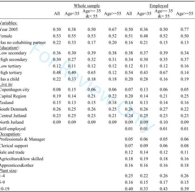
Finally, we control for additional individual and work characteristics, such as gender, cohabiting with a partner, presence of children in the household, level of education, dummies for plant size, as well as sectoral dummies and occupational dummies (for the employed only).

Descriptive Statistics

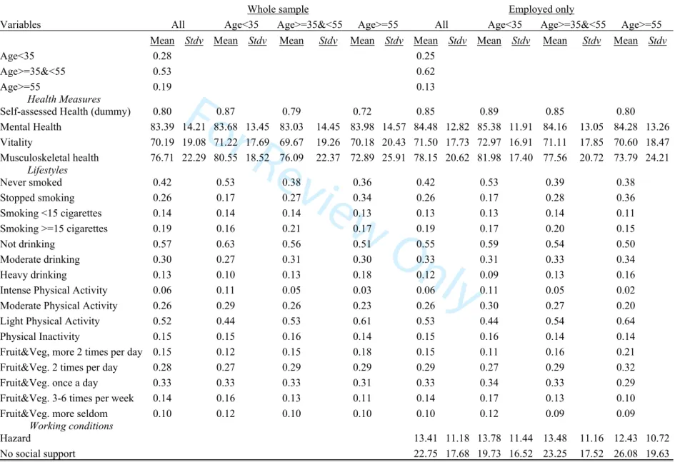
Table 1 describes the main variables for the entire sample and for the sub-sample of the employed and by age groups. Additional covariates are described in the Appendix A, Table A1. Of the 9,240 total observations, 28 percent refer to individuals less than 35 years old, about 53 percent between 35 and 54 and about 20 percent to those aged 55 or more.

<Table 1 here>

In the whole sample, almost 80 percent self-assess their perceived health as very good or good. The average MH is the highest and equals 83. VT is the lowest and equals about 70, while MSH is 77. In 42 percent of the cases, individuals have never smoked, 26 percent stopped smoking, while 14 percent currently smoke less than 15 cigarettes a day and 19 percent more than 15. In half of the cases, individuals do not drink on a daily basis and perform light physical activity. In 10 percent of

For Review Only

the cases, individuals drink heavily and do not eat fruit and vegetables. Around 15 percent reports being Physically Inactive and eating fruits and vegetables more than twice a day.

The percentage of individuals reporting very good and good health is 15 percent lower (72 percent) in the oldest group than in the youngest one (87 percent). Concerning specific health dimensions, differences by age are much smaller, except for MSH, which in the group of 55 and over is on average 7 points lower (73) than among people younger than 35 (80). Older individuals are more likely to be heavy drinkers. Smoking consumption is similar across age groups, while younger individuals are more likely to have never smoked and older individuals to have stopped smoking. Intense Physical Activity is more likely for younger individuals. Food habits are similar across age groups.

Employed people are 84 percent of the whole sample. They make up 91 percent of the 35 – 54 age range, 79 percent of the less-than-35 group and 70 percent of the group of older people.

The sub-panel of people employed in both 2000 and 2005 has 5,962 observations. The proportion of those aged 55 or more is lower than in the total sample (13 percent instead of 19, corresponding to 789 observations), while that of those in the middle age class is higher (62 percent instead of 53). The employed are, on average, more likely to have a good or very good SAH (85 percent). They have very similar VT, MH and MSH to people in the whole sample. At the descriptive level, there is little evidence that in Denmark the employed are healthier than the entire population. Health and lifestyle differences by age mimic those of the total sample, also in the group of older individuals.

With respect to working conditions, the highest average is for having No influence (in decisions), followed by No Repetitive(ness of) work, No social support and Hazards. In about one third of cases, individuals feel insecure about their job. Older workers perceive less social support and are more likely (43 percent) to be insecure about their job than younger ones (26 percent in the less-than-35 group). They are less likely to feel as having No influence on their work.

For Review Only

Model

In the baseline model, age effects in health do not depend on observable characteristics: [1] 𝐻𝑖𝑡= 𝛼1+ 𝛼2𝐴𝐺𝐸2𝑖𝑡+ 𝛼3𝐴𝐺𝐸3𝑖𝑡+𝛽𝐿𝑆𝑖𝑡+𝛾𝑊𝐶𝑖𝑡+ 𝑎𝑖+ 𝑢𝑖𝑡

is the health of the i-th worker at time t and can be either MH, VT, MSH or the SAH dummy. 𝐻𝑖𝑡

For the latter, Eq. [1] is a linear probability model. We leave implicit the inclusion of additional covariates and a time dummy. 𝐿𝑆𝑖𝑡 includes the set of lifestyles, 𝑊𝐶𝑖𝑡 the adverse working conditions. Age effects are captured by two dummies for people aged 35– 54 (AGE2) and 55 or more (AGE3). The excluded category is people less than 35 years old. The individual intercept 𝑎𝑖 controls for time-invariant individual unobservables. Jones et al. (2013) estimate a constrained version of Eq. [1] not controlling for lifestyles and using cross sectional data.

The second model consists of separate health equations by age groups:

, j = less than 35; 35-54; 55 and more. [2] 𝐻𝑖𝑗𝑡= 𝛼𝑗+ 𝛽𝑗𝐿𝑆𝑖𝑡+ 𝛾𝑗𝑊𝐶𝑖𝑡+ 𝑎𝑖𝑗+ 𝑢𝑖𝑗𝑡

and are age-specific gradients of lifestyles and working conditions. 𝛽𝑗 𝛾𝑗

There are several threats to the causal estimation of Eqs. [1] and [2]. First, individuals may endogenously sort into risky lifestyles or jobs. For example, healthier workers may be more likely in jobs that require higher physical and mental resilience. The second threat is that if healthier workers self-select into employment (‘healthy worker effect’) health effects computed in the sample of the employed would underestimate true effects. This may be relevant especially for older workers (see Li and Sung 1999 for a review). Jones et al. (2013) find a more negative work-related health impact of age once accounting for self-selection. Similarly, self-selection may affect also the estimation of WC variables, which are observed only in the sub-population of the employed.

Finally, the probability of being in the 2005 sample may correlate with health or lifestyles and working conditions. In the robustness analysis we address panel attrition using an Inverse Probability Weights (IPW) approach as in Mazzonna and Peracchi (2017).

For Review Only

We first estimate the health equations [1] and [2] by benchmark random effects (RE). They are affected by selectivity issues if unobserved heterogeneity correlates with 𝐿𝑆 and 𝑊𝐶 and/or with being employed. We then use the Mundlak’s correlated random-effects estimator (CRE) to account for time-invariant individual heterogeneity, specified as a linear function of within-individual means of all the included regressors plus an unobserved time-invariant individual component independent of them. The CRE estimator adds the within-individual means of the observed variables to the regressors, and it is therefore similar to the conventional fixed effects/within estimator.

We use CRE instead of fixed effects because of their higher flexibility, which facilitates the implementation of a number of extensions that are key to testing the robustness of our results. For example, CRE can incorporate correction-terms to control for self-selection into employment due to time-varying unobservables, as well as IPWs to control for attrition.

The main limitation of CRE is that it is not consistent if time-varying unobservables correlate with risky lifestyles and adverse working conditions. This may happen if, for example, current or past health shocks feedback on future values of key explanatory variables, perhaps differently across age groups.3 _{While we acknowledge the limitation of ignoring the endogeneity issue, we} leave a proper treatment of selection on time-varying unobservables - maybe with a more parsimonious specification in terms of LS and WC and different data - for our future research agenda. We abstract from that and take advantage of the richness of our data without claiming a causal interpretation for our results.4

5. Results

5.1. Model with age dummies

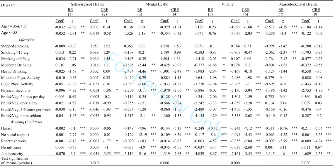
Table 2 shows the estimates of Eq. [1]. We report an average marginal effect of key explanatory variables on the probability of good or very good health (SAH) and on the 0-100 health indexes (MH, VT and MSH). We interpret these effects in terms of standard deviations or means of the variables of interest. Full results are in Table B1 of the on-line Appendix B.

For Review Only

Benchmark RE results (in odd columns) confirm that, with few exceptions, all working conditions are significant negative determinants of health. This is consistent with both theory and intuition and complements the analysis of Jones et al. (2013) who find similar results for work-related health. For example, job insecurity is associated with a 7 percent reduction in the probability of reporting good/very good SAH and with a roughly 3.7 percent (average marginal effect = -3.116*100/84.48 = mean of MH) reduction in MH.

Similarly to Cottini and Ghinetti (2017), we find that also lifestyles matter for health. They are all statistically associated with a lower level of VT. In the case of SAH and MH, only do very bad habits matter. For example, being physically inactive lowers SAH by almost 10 percent and MH (at its mean) by roughly 2.5 percent. The magnitude of marginal effects is smaller compared to working conditions.

Our main interest is in the health differentials by age. Workers aged 55 or more report significantly lower levels of SAH (-5.2 percent), better MH and lower MSH (-4.4 percent, at its mean) than those younger than 35. In the case of SAH and MSH this is true also for workers between 35 and 55 years of age. Conversely, VT does not show any statistical association with age. Results for MH and MSH are qualitatively comparable to Jones et al. (2013) for Europe and Davies

et al. (2016) for the UK.

Correlated random effects account for endogeneity and self-selection into employment due to time-constant unobserved heterogeneity. A test of joint significance of the means is equivalent to the Hausman test, and it may help in deciding which model – RE vs CRE – is more appropriate. It is shown in the last row of Table 2. The Hausman statistics are informative if, conditional on their means, all included regressors are exogenous. While in our case this assumption is questionable, the test suggests a clear violation of the RE assumption for all health outcomes, and provides empirical support to CRE instead of RE. Also Henseke (2018) and Jones et al. (2013) find that unobserved heterogeneity plays a role for estimated relationships.

For Review Only

In the case of adverse working conditions, CRE coefficients (in even columns) maintain their statistical significance, except for SAH, where the only dimension that matters is Job insecurity. As for lifestyles, CRE generally attenuates estimated effects. Only Physical inactivity maintains a negative and statistically significant relationship with each health measure. Average marginal effects indicate a reduction in SAH by 5.3 percent and a health loss of about 7.2 percent for individuals endowed with average VT (71.5). These results are similar to those of Humphreys et al. (2014) for Canada.

Age differentials are now smaller (in absolute terms) or insignificant. We do not observe substantial health penalties for older workers, except in the case of VT. In this respect, our results for Denmark are different from what has been found for the UK (see Davies et al., 2016; Jones et

al., 2013). This suggests that individual sorting mechanisms may substantially differ even between

countries where age-health gradients are similar. This may not be negligible and may have implications for public policies. In our case, the vanishing of health differentials by age may have alternative explanations. It could genuinely signal that unobserved fixed traits of older employed workers make them more likely to sort endogenously into the group with lower (SAH and MSH) or higher (MH and VT) health. Only the second case supports a ‘healthy worker effect’ interpretation. Another possibility is that, given the subjectivity of our health variables, time-invariant unobservables make older workers more likely to under (SAH and MSH) or over-report (MH and VT) true health.5

The online Appendix B documents and discusses additional results, which we briefly summarise hereafter. First, we exploit that the information on health and lifestyles is available for the entire sample, not only for the employed, and find that the endogenous sorting captured by time invariant heterogeneity is similar in the two groups. This excludes that older employed workers are healthier than same age not employed individuals. Second, by excluding potentially endogenous job controls (size, occupation and sector) from the baseline, we do not detect peculiar interactions between main regressors and covariates.

For Review Only

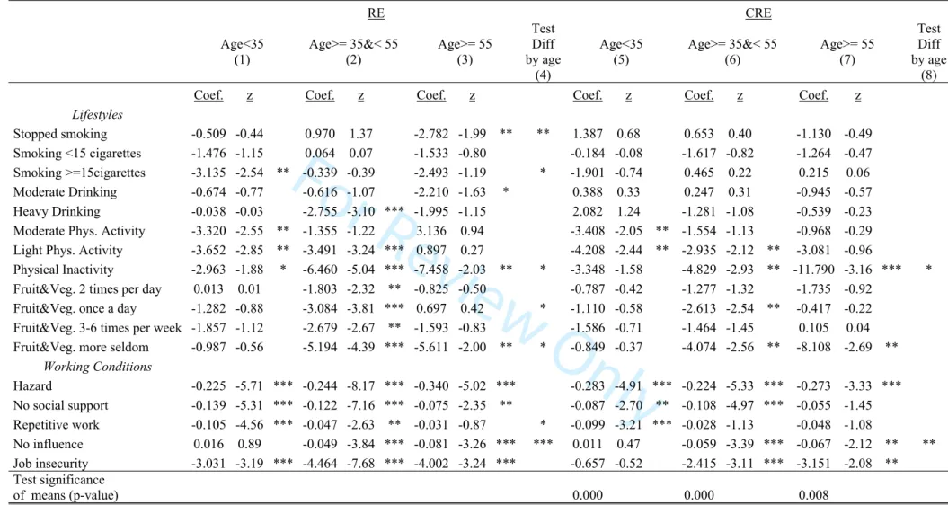
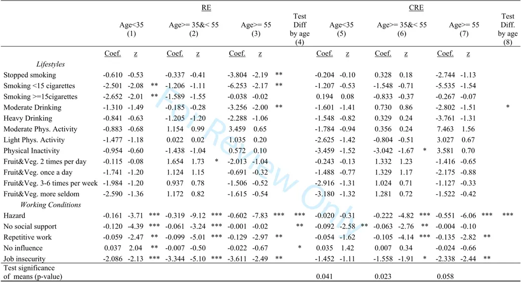
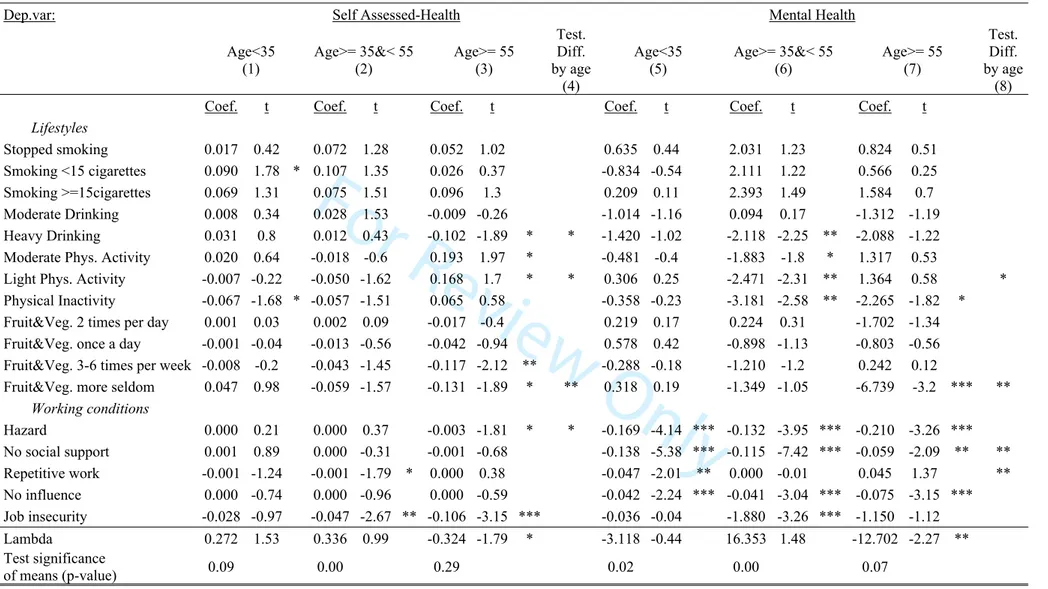
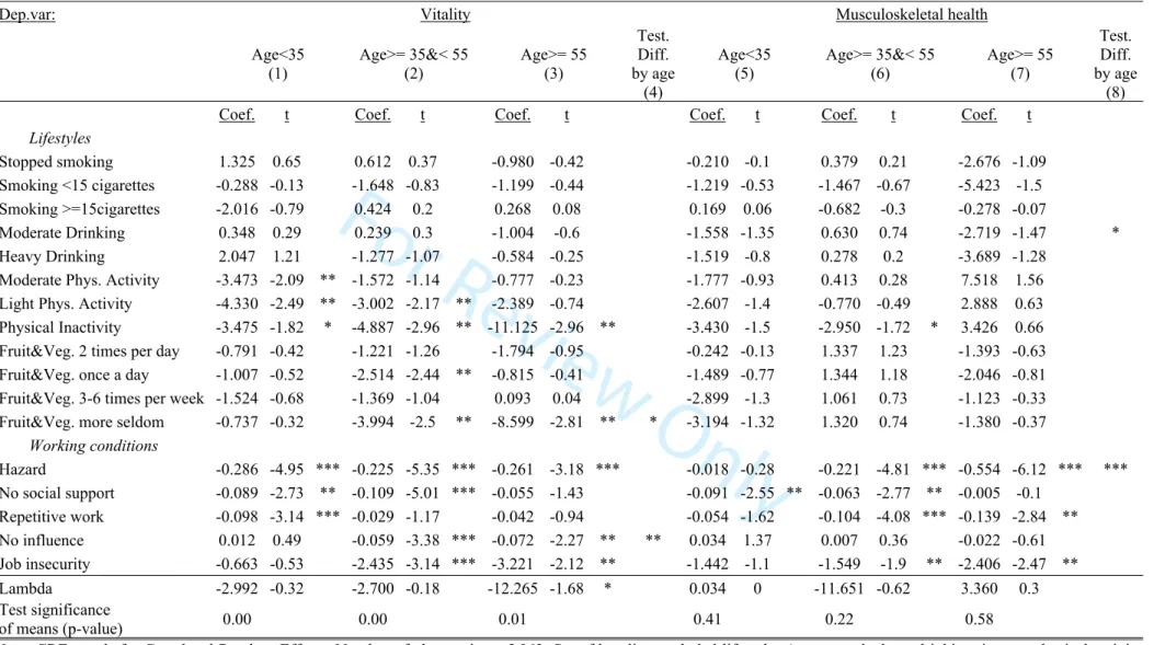
5.2. Separate equations by age

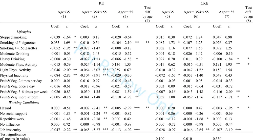
Table 3 presents RE and CRE estimates of age-specific health equations of Eq. [2]. In columns (1) and (5) we report results for individuals below 35 years of age, in columns (2) and (6) between 35 and 55 years of age and in columns (3) and (7) above 55 years of age.

In general, the overview of Table 3 suggests similar health gradients of lifestyles and working conditions by age. Indeed, for most LS and WC we do not reject the equality of coefficients across age groups.

<Table 3 here>

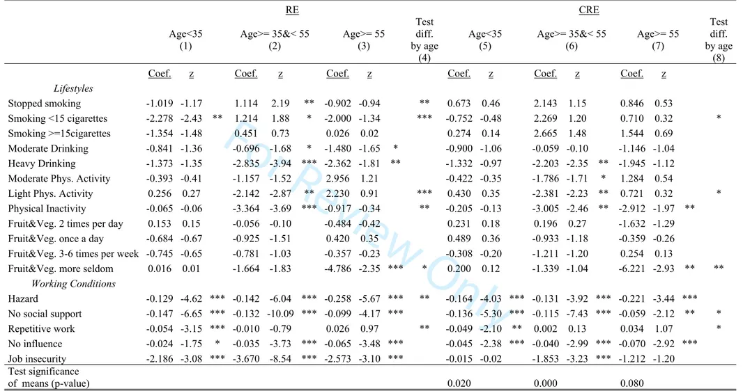
As for lifestyles, differences by age exist in MH and VT especially for smoking and dietary habits, and for physical activity. The lack of consumption of fruit & vegetables is particularly detrimental for people aged 55 or more, while it has no implications for the health of people aged 34 or less. Concerning Physical inactivity, our findings suggest that it implies a reduction of nearly 11 percent in VT (at its mean) for employees aged 55 or older. This effect is around one third for individuals aged under 35 (-4 percent). Similarly, the lack of a regular consumption of fruit and vegetables is associated with a nearly 6 percent lower MH of people older than 55 and 8 percent lower VT. As in Henseke (2018), we find that most health dimensions negatively relate to the adverse work conditions of older workers. However, our results also show that in many cases the effects for the two younger groups are similar. There are some noticeable exceptions. On the one hand, adverse physical work conditions (negatively) matter more for older workers than for younger ones. In particular for job hazards, and especially for MH and MSH. For example, a higher exposure is associated with relatively (to the younger age groups) lower MSH starting from prime age (35-55), and even more at older ages (55 and over), for whom the negative coefficient is twice (0.60) than that of people aged 35 – 55 (0.32).

Instead, younger workers suffer especially from adverse psychosocial working conditions. For example, their MH is more negatively affected by a lack of social support and by doing Repetitive

For Review Only

work than that of older counterparts. Interestingly, Job insecurity is an important determinant of health at all ages, but without clear age-specific patterns.

A visual inspection of Table 3 suggests that CRE results are overall qualitatively similar to RE, except that the subset of statistically significant differences by age groups is even narrower, perhaps reflecting differences in fixed individual unobserved traits. In terms of lifestyles, this is true for seldom consumption of fruit & vegetables on SAH, MH and VT, and for Light or Moderate Physical activity on MH and SAH. In absolute terms, the differences are not negligible. For example, the lack of a regular consumption of fruits and vegetables is associated with a nearly 12 percent lower MH of people older than 55, which is twice than that for RE. If we consider that effects may cumulate by adopting clusters of risky lifestyles, our results predict that older people with bad habits in food consumption and physical activity experience on average 28 percent less VT (11.2+17 percent due, respectively to bad food habits and physical inactivity) than same age more active and good eating peers. The VT implications of the same behaviours are halved for middle age workers (5.6+7 percent) and disappear at younger ages.

We spot some statistically significant differences by age also with respect to drinking and smoking behaviour, and in a few cases for working conditions. For example, age matters for Hazards on SAH and MSH, for Repetitive Work and No social support on MH. An increase of one standard deviation in Hazard (10.7) is associated with – 8 percent in MSH for people aged 55 or more. By converse, feeling less social support by one standard deviation implies a 3 percent reduction of VT in the group of younger workers (at its mean) and of 1.5 percent in the older group.

Extensions to the analysis of Table 3 are briefly summarised here and discussed in more detail in the online Appendix B. First, we use the number of cigarettes and drinks as alternative measures for smoking and drinking. We find a negative association between MH and drinking, in particular for workers aged 55 or more: 10 drinks or more are associated with 14 points less in MH. Second, we explore differences by gender, which are not substantial. Third, we exploit the ordered nature of the original survey question on self-assessed health and show that results are driven by people reporting

For Review Only

the highest level of health. Finally, we estimate health equations with 5 year lags in working conditions and lifestyles, which account for the fact that health consequences may take time to manifest. Differently from Henseke (2018), past lifestyles and working conditions maintain their negative correlation with current health, but their statistical significance is lower.

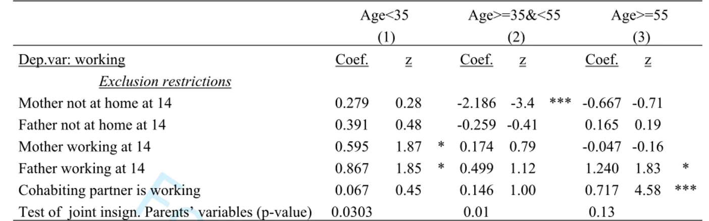
Robustness analysis

CRE results for the employed are representative of all workers only if time-invariant individual effects fully capture self-selection into employment. We allow for selectivity on time-varying unobservables through a two-step Heckman approach (Wooldridge 2005). In the first step, we estimate one CRE probit for each age group. We then use results to compute age-specific Heckman lambdas. These are included in the second step as additional regressors in augmented health equations estimated by CRE. Following Jackle and Himmler (2010), we use family characteristics as exclusion restrictions: a dummy for the labour market status of the cohabiting partner (if any); two dummies for the parents’ occupational status when the individual was 14, available only for parents who were present at home; two dummies to control for their presence or not. We assume that, ceteris paribus, labour market decisions of parents during adolescence and of the partner affect employment choices without any residual impact on an individual’s health.

First step probit coefficients show that for the two younger age groups parents’ variables are jointly statistically significant at the 5 percent level (see Table A2). Having an employed cohabiting partner increases the probability of working, but this is statistically significant only for older workers. Overall, many excluded variables do not strongly relate with the propensity to be employed. This is problematic especially for younger workers, since no exclusion restriction is individually statistically significant at 5 percent. This implies that the interpretation of the second step results of Table A3 requires particular care. The lambda terms are not statistically significant for the two younger groups. In the older age group, lambdas are negative and somehow statistically significant except for MSH. This suggests that the selection of older workers into employment is

For Review Only

reduction in the probability of employment. Again, this is in contrast with a healthy worker effect interpretation. Correcting for self-selection on time-varying unobservables does not alter the estimates of main parameters: selectivity-adjusted CRE coefficients are almost equivalent to the unadjusted CRE results of Table 3.

We re-estimate the CRE specification also using Inverse Probability Weights that allow attrition to depend on observable characteristics. We first estimate a probit for participation in the 2005 wave by conditioning on the value of the variables observed in the first wave, including health and lifestyles. The results (available upon request) indicate that, indeed, individuals with poor health or risky lifestyles are less likely to participate in the second round. Second, we use the inverse of the fitted probability to construct the weights we use in the estimations. Weighted estimates do not lead to substantially different results and are reported in the online Appendix B (see Table B8). Because our weights use important observable information, such as initial health, we conjecture that unobservables driving the attrition process may not substantially change our results.

6. Discussion and conclusion

The aim of this study is to analyse differences in health between older and younger workers and the contribution of adverse working conditions and risky lifestyles to them. We use a rich panel dataset of Danish inhabitants in their working age for 2000 and 2005. We consider three age groups: 18 – 34, 35 – 54, 55 and older. Our outcomes are indexes describing perceptions of SAH, MH and MSH and VT. We use a broad range of individual and employment characteristics including detailed information on adverse working conditions and risky lifestyles. The longitudinal dimension of the data and the availability of information on both employed and non-employed workers allow us to control for several selection mechanisms.

RE estimates show that older workers (especially in the 55 or older group) have lower SAH and MSH, and higher MH. We find no differences in terms of VT. Next, once we control for fixed unobservable individual traits, perceived levels of health (in terms of SAH, MH, MSH) are not statistically different across age groups, with the exception of VT, which is lower in the older

For Review Only

group. This suggests that failure to consider unobserved heterogeneity issues may result in erroneous conclusions on age-health gradients. Moreover, the direction of the error depends on the health measure considered. Overall, we do not find systematic evidence that healthier individuals tend to endogenously sort into employment, not even in the group of older workers. In this respect, our results for Denmark are somehow different from previous evidence from other countries.

Second, lifestyles and, especially, working conditions are significant determinants of health, but, at the same time, their contribution to health differentials by age is not systematic. In terms of risky lifestyles, only bad dietary habits and physical inactivity seem to matter, as they penalise more the health of older workers than that of younger ones. Furthermore, this is limited to MH and VT. Adverse working conditions negatively correlate with health, but similarly across age groups. The only difference is that adverse physical work conditions matter more for older workers; instead, younger workers suffer more from adverse psychosocial working conditions, such as a lack of social support and the repetitiveness of work.

While our data have a number of strengths, some limitations are worth mentioning. Since we are not able to fully control for time-varying unobservables, our estimates describe robust associations rather than a causal relationship. Second, the shortness of our panel does not allow us to model adequately persistence. If the effects of risky choices accumulate over time, older individuals could suffer more from them, independently of current behaviours. Further research that exploits longer time spans of data and adequate exclusion restrictions would ease a deeper investigation of such phenomena and nicely complement the findings reported herein.

On the policy side, our results suggest that older Danish workers who remain in employment do not appear intrinsically healthier than those not employed. This itself may be the result of Denmark being a leader in terms of health & safety at work at all ages and of the policies introduced for this purpose. Developing and adopting similar measures may help other countries to facilitate employment at older ages without health penalties, especially in terms of MH and MSH.

For Review Only

Our results also suggest that the design of policies aimed at favouring the well-being of workers at all ages is complex. First, interventions should be broad in terms of both health dimensions and risk factors, the latter having different implications depending on the health dimension considered. Second, policies that target specific age groups may require very narrow interventions and concern only certain health dimensions. We document these findings for Denmark, but the main policy implications are perhaps sufficiently general to apply to other countries and institutional settings.

Notes

1. In 2005, the questions for neck and shoulder were collapsed into a single question, but average Musculoskeletal Health is very similar for 2000 and 2005.

2. These are the Big four lifestyles that the US National Heart, Lung, and Blood Institute (NHLBI) indicated as able to prevent chronic diseases in adulthood.

3. Using instrumental variables would help to solve the problem, but this would require a very large set of exclusion restrictions, at least one for each element of the LS and WC vectors.

4. Reverse causality and endogeneity problems due to time-varying unobservables may be addressed using a selection on observables approach. For example, Bockerman et al. (2012) use sickness absence and work histories to capture unobserved health and risk preferences correlated with endogenous High Involvement Management practices. Unfortunately, we do not have access to all this information (including lifestyle histories) in our data.

5. This may happen, for example, because they evaluate their health using as reference their (higher) health when they were younger. Another reason might be the presence of cohort-effects in health.

References

Balia, S. and Jones, A. M. (2008). Mortality, lifestyle and socio-economic status. Journal of

Health Economics, 27: 1-26.

Barslund, M. (2015). Extending working lives: the case of Denmark. Centre for European Policy Studies Working Document no.404.

Bevan, S., Quadrello, T., McGee, R., Mahdon, M., Vavrovsky A. and Barham, L. (2009). Fit for

work? Musculoskletal disorders in the European Workforce. The Work Foundation.

Bland, J. M., and Altman, D. G. (1997). Statistics notes: Cronbach's alpha. British Medicine

Journal, 314: 275.

Bockerman, P. and Illmakunns, P. (2009). Job Disamenities, Job Satisfaction, Quit Intentions, and Actual Separations: Putting the Pieces Together. Industrial Relations, 48: 73-96.

Bockerman, P., Bryson, A. and Ilmakunnas, P. (2012). Does high involvement management improve worker wellbeing? Journal of Economic Behavior and Organization, 84: 660-680.

For Review Only

Borg, V. and Kristensen, T. S. (2000). Social class and self-rated health: Can the gradient be explained by differences in life style or work environment? Social Science and Medicine, 51: 1019-1030.

Brach, J. S., Simonsick, E. M., Kritchevsky, S., Yaffe, K. and Newman, A. B. (2004). The association between physical function and lifestyle activity and exercise in the Health, Aging and Body Composition Study. Journal of the American Geriatrics Society, 52: 502–9.

Burr, H., Albertsen, K., Rugulies, R. and Hannerz, H. (2010). Do dimensions from the Copenhagen Psychosocial Questionnaire predict vitality and mental health over and above the job strain and effort–reward imbalance models? Scandinavian Journal of Public Health, 38: 59-68.

Burr, H., Bjorner, J. B., Kristensen, T. S. and Tüchsen F, Bach, E. (2003). Trends in the Danish work environment in 1990–2000 and their associations with labor-force changes. Scandinavian

Journal of Work and Environmental Health, 29:270–279.

Cai, L. and Kalb, G. (2006). Health status and labour force participation: evidence from Australia. Health Economics, 15: 241-261.

Contoyannis, P. and Jones, A. M. (2004). Socio-economic status, health and lifestyle. Journal of

Health Economics, 23: 965-995.

Cottini, E. and Ghinetti, P. (2017). Is it the Way You Live or the Job You Have? Health Effects of Lifestyles and Working Conditions. The B.E. Journal of Economic Analysis & Policy, 17(3).

Cottini, E. and Lucifora, C. (2013). Mental Health and Working Conditions in European Countries. Industrial and Labor Relations Review, 66: 958-988.

Cox, T., Griffiths, A. and Rial-González, E. (2000). Research on work-related stress. Luxembourg: European Agency for Safety and Health at Work.

Cuijpers, P., Smits, N., Donker, T., ten Have, M., de Graaf, R. (2009). Screening for mood and anxiety disorders with the five-item, the three-item, and the two item mental health inventory.

Psychiatry Research, 168:250–255.

Datta Gupta, N. and Kristensen, N. (2007). Work environment satisfaction and employee health: panel evidence from Denmark, France and Spain, 1994-2001. European Journal of Health

Economics, 9:51-61.

Davies, R., Jones, M. and Lloyd-Williams, H. (2016). Age and Work related health: insights from the UK Labour Force Survey. British Journal of Industrial Relations, 54:136-159.

Feveile, H., Olsen, O. and Hogh, A. (2007) A randomized trial of mailed questionnaires versus telephone interviews: response patterns in a survey. BMC Medical Research Methodology, 7:27.

Fletcher, J.M., Sindelar, J. L. and Yamaguchi, S. (2011). Cumulative effects of job characteristics on health. Health Economics, 20:553-570.

Green, F. and Mostafa, T. (2012). Trends in job quality in Europe. European Union, Luxemburg. Henseke, G. (2018). Good Jobs, good pay, better health? The effects of job quality on health among older European workers. European Journal of Health Economics, 19:59–73.

Hu, T. W., Ren, Q. F., Keeler, T. and Bartlett, J. (1995). The demand for cigarettes in California and behavioural risk factors. Health Economics, 4:7-14.

For Review Only

Humphreys, B.R., Mcleod, L. and Ruseski, J. E. (2014). Physical Activity and health outcomes: evidence from Canada. Health Economics, 23:33-54.

Jackle, R. and Himmler, O. (2010). Health and Wages: Panel Data Estimates Considering Selection and Endogeneity. Journal of Human Resources, 45: 64-40.

Jones, M., Latreille, P., Sloane, P. and Staneva, A. (2013). Work-related health risks in Europe: Are older workers more vulnerable? Social Science & Medicine, 88:18-29.

Jurges, H. (2007). True health vs Response Style: exploring cross country differences in self-reported health. Health Economics, 16: 163–178.

Karasek, R. and Theorell, T. (1990). Healthy work: stress, productivity, and the reconstruction of working life. New York: Basic Books.

Kenkel, D. (1991). Health Behavior, Health Knowledge, and Schooling. The Journal of Political

Economy, 2: 287-305.

Kenkel, D. (1995). Should you eat breakfast? Estimates from health production functions.

Health Economics, 4: 5-29.

Kristensen, T.S., Borg, V. and Hannerz, H. (2002). Socioeconomic status and psychosocial work environment: results from a Danish national study. Scandinavian Journal of Public Health, 30: 41-48.

Kristensen, T.S., Hannerz, H. and Borg, V. (2005). The Copenhagen Psychosocial Questionnaire – a tool for the assessment and improvement of the psychosocial work environment. Scandinavian

Journal of Work, Environment & Health, 31: 438-449.

Kuorinka, I., Jonsson, B., Kilbom, A., Vinterberg, H., Biering-Sørensen, F., Andersson, G. and Jørgensen, K. (1987). Standardized Nordic questionnaires for the analysis of musculoskeletal symptoms. Applied Ergonomics, 18:233–237.

Li, C. and Sung, F. (1999). A review of the healthy worker effect in occupational epidemiology.

Occupational Medicine, 49: 225-229.

Loef, M., Walach, H. (2012). The combined effects of healthy lifestyle behaviors on all causes of mortality: a systematic review and meta-analysis. Preventive Medicine, 55:163–170.

Mazzonna, F. and Peracchi, F. (2017). Unhealthy Retirement. Journal of Human Resources, 52(1): 128-151.

Netterstrøm, B., Kristensen, T.S., Damsgaard, M.T., Olsen, O. and Sjol, A. (1991). Job strain and cardiovascular risk factors: a cross sectional study of employed Danish men and women.

British Journal of Industrial Medicine, 48: 684-689.

Osler, M., Heitmann, B.L., Hoidrup, S., Jørgensenb, L.M. and Schroll, M. (2001). Food intake patterns, self rated health and mortality in Danish men and women. A prospective observational study. Journal of Epidemiology Community Health, 55:399–403.

Patja, K., Jousilahti, P., Hu, G. and Valle, T. (2005). Effects of smoking, obesity and physical activity on the risk of type 2 diabetes in middle-aged Finnish men and women. Journal of Internal

Medicine, 258:356-362.

Rice, N.E., Lang, I.A., Henley, W. and Melzer, D. (2010). Common health predictors of early retirement: findings from the English longitudinal study of ageing. Age and Ageing, 40: 54–61.

For Review Only

Robone, S., Jones, A.M. and Rice, N. (2011). Contractual conditions, working conditions, health and well-being in the British Household Panel Survey. European Journal of Health Economics, 12: 429-444.

Rugulies, R., Bultmann, U., Aust, B., Burr, H. (2006). Psychosocial work environment and incidence of severe depressive symptoms: prospective findings from a 5-year follow-up of the Danish Work Environment Cohort Study. American Journal of Epidemiology, 163:877–87.

Rumpf, H.J., Meyer, C., Hapke, U., John, U. (2001). Screening for mental health: validity of the MHI-5 using DSM-IV Axis I psychiatric disorders as gold standard. Psychiatry Research, 105:243– 253.

Schmitz, L. (2016). Do working conditions at older ages shape the health gradient? Journal of

Health Economics, 50: 183–197.

Siegrist, J. (1996). Adverse Health Effects of High-Effort/Low-Reward Conditions. Journal of

Occupational Health Psychology, 1: 27-41.

Siegrist, J. and Rödel, A. (2006). Work stress and health risk behavior. Scandinavian Journal of

Work, Environment & Health, 32: 473-481.

Ware, J.E. and Gandek, B. (1998). Overview of the SF-36 Health Survey and the International Quality of Life Assessment (IQOLA) Project, Journal of Clinical Epidemiology, 51: 903-12.

Wooldridge, J. (2005). Econometric Analysis of Cross Section and Panel Data. Second Edition. The MIT Press, Cambridge, Massachusetts.

For Review Only

Table 1: Descriptive Statistics (main variables)

Whole sample Employed only

Variables All Age<35 Age>=35&<55 Age>=55 All Age<35 Age>=35&<55 Age>=55 Mean Stdv Mean Stdv Mean Stdv Mean Stdv Mean Stdv Mean Stdv Mean Stdv Mean Stdv

Age<35 0.28 0.25

Age>=35&<55 0.53 0.62

Age>=55 0.19 0.13

Health Measures

Self-assessed Health (dummy) 0.80 0.87 0.79 0.72 0.85 0.89 0.85 0.80 Mental Health 83.39 14.21 83.68 13.45 83.03 14.45 83.98 14.57 84.48 12.82 85.38 11.91 84.16 13.05 84.28 13.26 Vitality 70.19 19.08 71.22 17.69 69.67 19.26 70.18 20.43 71.50 17.73 72.97 16.91 71.11 17.85 70.60 18.47 Musculoskeletal health 76.71 22.29 80.55 18.52 76.09 22.37 72.89 25.91 78.15 20.62 81.98 17.40 77.56 20.72 73.79 24.21 Lifestyles Never smoked 0.42 0.53 0.38 0.36 0.42 0.53 0.39 0.38 Stopped smoking 0.26 0.17 0.27 0.34 0.26 0.17 0.28 0.36 Smoking <15 cigarettes 0.14 0.14 0.14 0.13 0.13 0.13 0.14 0.11 Smoking >=15 cigarettes 0.19 0.16 0.21 0.17 0.19 0.17 0.20 0.15 Not drinking 0.57 0.63 0.56 0.51 0.55 0.59 0.54 0.50 Moderate drinking 0.30 0.27 0.31 0.30 0.33 0.31 0.33 0.34 Heavy drinking 0.13 0.10 0.13 0.18 0.12 0.09 0.13 0.16 Intense Physical Activity 0.06 0.11 0.05 0.03 0.06 0.11 0.05 0.02 Moderate Physical Activity 0.26 0.29 0.26 0.23 0.26 0.30 0.27 0.20 Light Physical Activity 0.52 0.44 0.53 0.61 0.53 0.44 0.54 0.64 Physical Inactivity 0.15 0.15 0.16 0.14 0.15 0.16 0.14 0.14 Fruit&Veg, more 2 times per day 0.15 0.12 0.15 0.18 0.15 0.11 0.16 0.21 Fruit&Veg. 2 times per day 0.28 0.27 0.29 0.29 0.29 0.27 0.29 0.32 Fruit&Veg. once a day 0.33 0.33 0.33 0.31 0.33 0.34 0.33 0.29 Fruit&Veg. 3-6 times per week 0.14 0.16 0.13 0.11 0.14 0.17 0.13 0.10 Fruit&Veg. more seldom 0.10 0.12 0.10 0.10 0.10 0.12 0.09 0.09

Working conditions

Hazard 13.41 11.18 13.78 11.44 13.48 11.16 12.43 10.72 No social support 22.75 17.68 19.73 16.52 23.25 17.52 26.08 19.63

For Review Only

For Review Only

Table 2: Health estimates on the employed. Random Effects (RE) and Correlated Random Effects (CRE)

Dep.var: Self-assessed Health Mental Health Vitality Musculoskeletal Health

RE (1) CRE (2) RE (3) CRE (4) RE (5) CRE (6) RE (7) CRE (8)

Coef. z Coef. t Coef. z Coef. t Coef. z Coef. t Coef. z Coef. t

Age>= 35&< 55 _{-0.032 -2.87 ** 0.003 0.14 0.136 0.34 -0.929 -1.21 0.129 0.23 -1.699 -1.68 * -2.572 -4.39 *** -1.184 -1.14} Age>= 55 _{-0.052 -2.81 ** -0.019 -0.58 1.326 2.18 ** -0.354 -0.32 0.645 0.76 -3.076 -2.03 ** -3.286 -3.3 *** -0.122 -0.07} Lifestyles Stopped smoking -0.009 -0.73 0.053 1.52 0.353 0.86 1.558 1.53 0.056 0.1 0.764 0.51 -0.995 -1.45 -0.200 -0.12 Smoking <15 cig. 0.003 0.22 0.089 1.29 -0.108 -0.21 1.189 0.99 -0.583 -0.83 -0.809 -0.47 -2.062 -2.37 ** -1.793 -0.93 Smoking >=15cig. -0.034 -2.21 ** 0.069 1.55 -0.195 -0.39 1.804 1.31 -1.418 -2.03 ** 0.107 0.06 -1.764 -2.12 ** -0.477 -0.23 Moderate Drinking 0.010 1.05 0.016 1.11 -0.805 -2.44 ** -0.425 -0.93 -0.777 -1.68 * 0.128 0.2 -0.801 -1.53 -0.372 -0.55 Heavy Drinking -0.025 -1.68 * 0.002 0.09 -2.474 -4.46 *** -1.901 -2.48 ** -1.983 -2.84 ** -0.169 -0.18 -1.124 -1.44 -0.558 -0.5 Moderate Phys. Activity -0.010 -0.65 0.007 0.33 -0.470 -0.79 -0.884 -1.13 -1.641 -1.98 * -2.086 -1.98 ** 0.379 0.44 -0.088 -0.08 Light Phys. Activity -0.051 -3.38 *** -0.023 -1.01 -0.989 -1.66 * -1.033 -1.27 -3.220 -3.94 *** -3.285 -3 *** -0.695 -0.8 -1.433 -1.18 Physical Inactivity -0.096 -4.92 *** -0.053 -1.86 * -2.206 -3.11 *** -1.970 -2.06 ** -5.886 -6.03 *** -5.170 -3.94 *** -1.486 -1.42 -2.753 -1.89 * Fruit&Veg. 2 times per day 0.006 0.45 -0.003 -0.2 -0.116 -0.24 -0.128 -0.21 -1.341 -2.06 ** -1.304 -1.59 0.722 0.94 0.560 0.62 Fruit&Veg. once a day -0.021 -1.52 -0.019 -0.99 -0.755 -1.51 -0.546 -0.84 -2.242 -3.33 *** -1.959 -2.28 ** 0.114 0.14 0.029 0.03 Fruit&Veg. 3-6 times per week -0.038 -2.15 ** -0.046 -1.93 ** -0.774 -1.28 -0.860 -1.05 -2.489 -3.07 *** -1.459 -1.35 -0.159 -0.16 -0.476 -0.4 Fruit&Veg. more seldom -0.041 -1.93 ** -0.028 -0.95 -1.515 -2.1 ** -1.360 -1.35 -4.135 -4.29 *** -3.358 -2.62 ** -0.140 -0.12 -0.287 -0.2

Working Conditions Hazard -0.002 -3.1 *** 0.000 -0.06 -0.148 -7.96 *** -0.144 -5.17 *** -0.248 -10.42 *** -0.243 -7.12 *** -0.311 -10.96 *** -0.211 -5.34 *** No social support -0.001 -2.77 ** 0.000 -0.01 -0.129 -12.19 *** -0.109 -8.59 *** -0.117 -8.6 *** -0.094 -5.43 *** -0.063 -4.22 *** -0.061 -3.23 *** Repetitive work -0.001 -2.12 ** -0.001 -1.77 * -0.020 -1.83 * -0.014 -0.95 -0.063 -4.52 *** -0.055 -2.84 ** -0.092 -5.79 *** -0.089 -4.24 *** No influence 0.000 -0.68 0.000 -1 -0.037 -4.9 *** -0.045 -4.05 *** -0.037 -3.7 *** -0.039 -2.68 ** 0.001 0.11 0.011 0.67 Job insecurity -0.070 -6.7 *** -0.051 -3.55 *** -3.116 -9.16 *** -1.319 -2.85 ** -4.039 -8.67 *** -2.161 -3.43 *** -3.145 -6 *** -1.689 -2.53 ** Test significance of means (p-value) 0.010 0.000 0.000 0.020

Note: RE stands for Random Effects. CRE stands for Correlated Random Effects. Number of observations: 5,962. All the regressions include a constant plus dummies for 2005. Set of baseline excluded lifestyles: never smoked, no drinking, intense physical activity, fruit & vegetables more than twice a day. Additional controls: female, education levels, having children, region, have no cohabiting partner, plant size, sector and occupation. z stands for z-statistics; t for t-statistics. In the CRE models we also include the mean of all included regressors. Robust standard errors are clustered at the individual level. *, **, *** indicate significance at the 10%, 5% and 1% level, respectively.

For Review Only

Table 3. Self-assessed Health estimates by age. Random Effects (RE) and Correlated Random Effects (CRE)

RE CRE

Age<35

(1) Age>= 35&< 55 (2) Age>= 55 (3)

Test diff by age

(4)

Age<35

(5) Age>= 35&< 55 (6) Age>= 55 (7)

Test diff. by age

(8) Coef. z Coef. z Coef. z Coef. z Coef. z Coef. z

Lifestyles Stopped smoking -0.039 -1.64 * 0.003 0.18 -0.020 -0.64 0.015 0.38 0.072 1.24 0.049 0.98 Smoking <15 cigarettes 0.035 1.69 * 0.010 0.54 -0.104 -2.10 ** ** 0.082 1.73 * 0.107 1.25 0.026 0.37 Smoking >=15cigarettes -0.052 -1.95 ** -0.028 -1.47 -0.008 -0.18 0.062 1.16 0.077 1.56 0.092 1.25 Moderate Drinking -0.001 -0.03 0.018 1.43 -0.015 -0.52 0.004 0.18 0.026 1.42 -0.006 -0.16 Heavy Drinking -0.008 -0.30 -0.022 -1.13 -0.066 -1.58 * 0.027 0.70 0.011 0.39 -0.100 -1.84 * * Moderate Phys. Activity -0.013 -0.59 -0.024 -1.14 0.136 1.53 0.019 0.62 -0.016 -0.51 0.191 1.93 ** * Light Phys. Activity -0.046 -2.09 ** -0.064 -3.07 *** 0.059 0.67 -0.010 -0.32 -0.047 -1.52 0.152 1.54

Physical Inactivity -0.084 -2.83 ** -0.104 -3.91 *** -0.029 -0.30 -0.072 -1.65 * -0.053 -1.40 0.048 0.43 Fruit&Veg. 2 times per day 0.000 -0.01 0.016 0.97 -0.015 -0.43 -0.001 -0.03 0.001 0.05 -0.014 -0.33 Fruit&Veg. once a day -0.016 -0.61 -0.017 -0.96 -0.021 -0.59 0.003 0.09 -0.015 -0.64 -0.031 -0.72 Fruit&Veg. 3-6 times per week -0.026 -0.83 -0.030 -1.35 -0.081 -1.59 * -0.007 -0.16 -0.043 -1.48 -0.116 -2.09 ** Fruit&Veg. more seldom -0.005 -0.16 -0.041 -1.48 -0.118 -1.98 ** 0.052 1.08 -0.059 -1.56 -0.117 -1.71 * *

Working Conditions Hazard 0.000 -0.51 -0.002 -2.41 ** -0.005 -2.99 *** ** 0.000 0.20 0.000 0.42 -0.003 -1.95 * * No social support -0.001 -1.83 * -0.001 -2.24 ** -0.001 -0.82 0.001 0.86 0.000 -0.26 -0.001 -0.69 Repetitive work -0.001 -1.48 -0.001 -2.18 ** 0.000 0.42 -0.001 -1.12 -0.001 -1.68 * 0.000 0.13 No influence 0.000 0.72 0.000 -0.78 -0.001 -0.99 0.000 -0.72 0.000 -0.98 0.000 -0.44 Job insecurity -0.047 -2.22 ** -0.068 -5.27 *** -0.113 -4.02 *** -0.028 -0.97 -0.046 -2.65 ** -0.107 -3.19 *** Test significance of means (p-value) 0.100 0.010 0.330

Note: RE stands for Random Effects. CRE stands for Correlated Random Effects. Number of observations: 1,474 (age<35); 3,699 (age>=35&age<55); 789 (age >=55). All the regressions include a constant plus dummies for 2005. Set of baseline excluded lifestyles: never smoked, no drinking, intense physical activity, fruit & vegetables more than twice a day. Additional controls: female, education levels, having children, region, have no cohabiting partner; plant size, sector and occupation. z stands for z-statistics; t for t-statistics. In the CRE models we also include the mean of all included regressors. Columns (4) & (8) report the statistical significance of testing that associated coefficients are different in the three age groups. Robust standard errors are clustered at the individual level. *, **, *** indicate significance at the 10%, 5% and 1% level, respectively.

For Review Only

Table 3: Mental Health estimates by age. Random Effects (RE) and Correlated Random Effects (CRE), (continued).

RE CRE

Age<35

(1) Age>= 35&< 55 (2) Age>= 55 (3)

Test diff. by age

(4)

Age<35

(5) Age>= 35&< 55 (6) Age>= 55 (7)

Test diff. by age

(8) Coef. z Coef. z Coef. z Coef. z Coef. z Coef. z

Lifestyles Stopped smoking -1.019 -1.17 1.114 2.19 ** -0.902 -0.94 ** 0.673 0.46 2.143 1.15 0.846 0.53 Smoking <15 cigarettes -2.278 -2.43 ** 1.214 1.88 * -2.000 -1.34 *** -0.752 -0.48 2.269 1.20 0.710 0.32 * Smoking >=15cigarettes -1.354 -1.48 0.451 0.73 0.026 0.02 0.274 0.14 2.665 1.48 1.544 0.69 Moderate Drinking -0.841 -1.36 -0.696 -1.68 * -1.480 -1.65 * -0.900 -1.06 -0.059 -0.10 -1.146 -1.04 Heavy Drinking -1.373 -1.35 -2.835 -3.94 *** -2.362 -1.81 ** -1.332 -0.97 -2.203 -2.35 ** -1.945 -1.12 Moderate Phys. Activity -0.393 -0.41 -1.157 -1.52 2.956 1.21 -0.422 -0.35 -1.786 -1.71 * 1.284 0.54

Light Phys. Activity 0.256 0.27 -2.142 -2.87 ** 2.230 0.91 *** 0.430 0.35 -2.381 -2.23 ** 0.721 0.32 * Physical Inactivity -0.065 -0.06 -3.364 -3.69 *** -0.917 -0.34 ** -0.205 -0.13 -3.005 -2.46 ** -2.912 -1.97 ** Fruit&Veg. 2 times per day 0.153 0.15 -0.056 -0.10 -0.484 -0.42 0.231 0.18 0.196 0.27 -1.632 -1.29 Fruit&Veg. once a day -0.684 -0.67 -0.925 -1.51 0.420 0.35 0.489 0.36 -0.933 -1.18 -0.359 -0.26 Fruit&Veg. 3-6 times per week -0.745 -0.65 -0.781 -1.03 -0.357 -0.23 -0.308 -0.20 -1.211 -1.20 0.254 0.13

Fruit&Veg. more seldom 0.016 0.01 -1.664 -1.83 -4.786 -2.35 *** * 0.200 0.12 -1.339 -1.04 -6.221 -2.93 ** **

Working Conditions Hazard -0.129 -4.62 *** -0.142 -6.04 *** -0.258 -5.67 *** ** -0.164 -4.03 *** -0.131 -3.92 *** -0.221 -3.44 *** No social support -0.147 -6.65 *** -0.132 -10.09 *** -0.099 -4.17 *** -0.136 -5.30 *** -0.115 -7.43 *** -0.059 -2.12 ** * Repetitive work -0.054 -3.15 *** -0.010 -0.79 0.026 0.97 ** -0.049 -2.10 ** 0.002 0.13 0.034 1.07 * No influence -0.024 -1.75 * -0.035 -3.73 *** -0.065 -3.48 *** -0.045 -2.38 *** -0.040 -2.99 *** -0.070 -2.92 *** Job insecurity -2.186 -3.08 *** -3.670 -8.54 *** -2.573 -3.10 *** -0.015 -0.02 -1.853 -3.23 *** -1.212 -1.20 Test significance of means (p-value) 0.020 0.000 0.080