Methods for the analysis of structural systems subjected to seismic acceleration modelled as stochastic processes

UNIVERSITÀ DEGLI STUDI DI MESSINA

Dipartimento di Ingegneria

Corso di Dottorato di Ricerca in

“Ingegneria e Chimica

dei Materiali e delle Costruzioni”

XXIX Ciclo

Methods for the analysis of structural

systems subjected to seismic acceleration

modelled as stochastic processes

Tesi di Dottorato di: Tiziana ALDERUCCI

Coordinatore:

Prof. Signorino GALVAGNO

Tutor:

Chiar.mo Prof. Ing.

Giuseppe MUSCOLINO

To my little daughter

Carlotta

Acknowledgments

It is very difficult for me to write these few words, since it means that my Ph.D. is coming to the end.

First of all my sincere thank goes to Professor Muscolino, who followed, supported (and tolerate!) me during these three years. It was a beautiful experience to work with him, since he continuously gave me ideas and suggestions for my study. Professor Muscolino contributed to my professional growth, making me “fall in love” with research.

An important thank goes to my family, major presence in my life; my parents always encouraged me, and they have spurred me to never give up.

Last, but not least, a special thank goes to my husband Sebastiano, who patiently waited for me every time that commitments made me come back home late.

Index

Summary ... 1

Chapter 1 - Preliminary definitions ... 5

1.1 Introduction ... 5

1.2 Random variables and random process ... 5

1.3 Stationary Gaussian random processes ... 9

1.4 Stationary spectral moments ... 12

1.5 Distribution of extreme values for stationary random process ... 16

Chapter 2 - Models of the ground motion acceleration process 21 2.1 Introduction ... 21

2.2 Real earthquakes... 26

2.3 The evolutionary process model ... 36

2.3.1 Definition of the non-stationary stochastic input ... 36

2.3.2 Models of the non-stationary random process ... 38

2.5 Adaptive chirplet decomposition ...45

2.6 Fully non-stationary spectrum compatible seismic waves ...48

2.6.1 Simulation of the random process samples ...48

2.6.2 Stationary spectrum-compatible accelerograms ...50

2.6.3 Non-stationary spectrum-compatible accelerograms ...52

2.7 Multi-correlated seismic input ...56

2.7.1 Introduction ...56

2.7.2 The evolutionary process model for multi-correlated input ...57

2.7.3 The sigma-oscillatory process model for multi-correlated input ...62

2.7.4 Simulation of non-stationary stochastic multi-correlated sigma-oscillatory vector processes ...68

2.8 Numerical Applications ...73

2.8.1 Fully non-stationary spectrum-compatible artificial earthquakes ...73

2.8.2 Multi-correlated seismic input...80

2.9 Summary and conclusions ...87

Chapter 3 - Spectral characteristics of the response ...91

3.1 Introduction...91

3.2 Classically damped structures subjected to mono-correlated input ...93

3.2.1 Equations of motion ...93

3.2.2 Stationary SMs……….…96

3.3 Classically damped structures subjected to multi-correlated input ... 102

3.3.1 Equations of motion ... 102

3.2.2 Evaluation of the NGSMs ... 104

3.4 Non-Classically damped structures subjected to mono-correlated input ... 109

3.4.1 Equations of motion ... 109

3.4.2 Evaluation of the NGSMs ... 111

3.5 Monte Carlo simulation for the evaluation of NGSMs ... 114

3.5.1 Classically damped structures subjected to mono-correlated input ... 115

3.5.2 Classically damped structures subjected to multi-correlated input ... 117

3.5.3 Non-Classically damped structures subjected to mono-correlated input ... 119

3.6 The Role of NGSMs in reliability analysis of structures ... 120

3.7 Summary and conclusions ... 122

Chapter 4 - Closed form solutions of the EPSD function matrix of the response ... 125

4.1 Introduction ... 125

4.2 Closed form solution of the EPSD matrix ... 127

4.2.1 Closed form solutions for classically damped structures subjected to mono-correlated input ... 127

4.2.2 Closed form solutions for classically damped structures

subjected to multi-correlated input ... 132

4.2.3 Closed form solutions for non-classically damped structures subjected to mono-correlated input ... 139

4.3 Numerical applications ... 143

4.3.1 Classically damped systems subjected to mono correlated input ... 143

4.3.2 Classically damped systems subjected to multi-correlated input ... 162

4.3.3 Non-classically damped system subjected to mono-correlated input... 168

4.4 Summary and conclusions ... 186

Chapter 5 - First passage probability problem ... 189

5.1 Introduction... 189

5.2 First passage probability problem: preliminary concepts... 193

5.2.1 Methods requiring the mean up-crossing rate of given thresholds ... 193

5.2.2 Methods requiring censored closures ... 198

5.3 Reliability assessment ... 203

5.4 Numerical Applications ... 205

5.4.1 Single-Degree of Freedom systems ... 205

5.4.2 Multi-Degrees of Freedom systems ... 211

Conclusions ... 229

Appendix A - TFR vector functions ... 233

A.1 Evolutionary process model ... 233

A.1.1 General solution ... 233

A.1.2 Normalized exponential type I modulating function.... 234

A.1.3 Normalized exponential type II modulating function .. 236

A.1.4 Normalized Jennings et al type modulating function .. 238

A.1.5 Spanos and Solomos model of the fully non-stationary process ... 241

A.2. Sigma-oscillatory process model ... 242

A.3 Adaptive chirplet decomposition ... 244

“Earthquakes systematically bring out the mistakes made in design and construction – even the most minute mistake; it is this aspect of earthquake engineering that makes it challenging

and fascinating, and gives it an educational value far beyond its immediate objectives”

Newland N.M. and Rosenblueth E. Fundamentals of earthquake

Summary

In the framework of the design and of the reliability assessment of fixed structures, among the static and dynamic loads that have to be considered, certainly the most important one is the seismic load, due to its terrible and disastrous consequences, not only in terms of the breakdown of the structure but also for the preservation of life. In fact during the past decades Italy has been the scene of terrible earthquakes, that destroyed whole cities and with a lot of human victims. First of all, in terms of magnitude and, unfortunately, a large number of deaths, Messina earthquake, in 1908, caused about 120000 victims, between Messina and Reggio Calabria, with an estimated magnitude of 7.1 (Richter scale). Then Irpinia earthquake, in 1980 (2914 victims, 6.5 Ricther), L’Aquila earthquake, in 2009 (309 victims, 5.9 Ricther) and the last events in 2016 in the centre of Italy, see Amatrice (299 victims, 6 Richter), Ussita (5.9 Richter), and Norcia (2 victims, 6.1 Ricther).

Due to the difficulty in the prevision of the seismic event, one of the most important and hard problem in seismic engineering is the correct characterization of the ground motion acceleration; in fact it has been demonstrated that it is possible to increase the reliability level of the structures defining in a suitable way the seismic input and shaping realistically the structure.

Nowadays, from the analysis of the large amount of data of recorded events, it is possible to study the main characteristics of real earthquakes and reproduce them with analytical models. In particular, because of the randomness of the seismic event, in terms of energy distribution and intensity, propagation path of the seismic waves through any specified location from the earthquake focus to the epicenter, etc…, it has been shown that it should be modelled as a stochastic process.

On the other hand, once the input has been defined, the second problem in the seismic engineering is the reliability assessment of the structures subjected to the ground motion acceleration. It is obvious that, if the excitations are modelled as random processes, the dynamic responses are random processes too, and the structural safety needs to be evaluated in a probabilistic sense. Among the models of failure, the simplest one, which is also the most widely used in practical analyses, is based on the assumption that a structure fails as soon as the response at a critical location exits a prescribed safe domain for the first time. In random vibration theory, the problem of probabilistically predicting this event is termed first

passage problem. Unfortunately, this is one of the most complicated

problem in computational stochastic mechanics. Therefore, several approximate procedures have been proposed. These procedures lead to the probabilistic assessment of structural failure as a function of barrier crossing rates, distribution of peaks and extreme values. The latter quantities can be evaluated, for non-stationary input process, as a function of the well-known Non-Geometric Spectral Moments (NGSMs).

Aim of this thesis is to propose a novel procedure to obtain closed form solutions of the spectral characteristics of the response of linear structural systems subjected to seismic acceleration modelled as

stochastic processes. The proposed method is a powerful tool in the analysis of both classically and non-classically damped systems, in reliability assessment problems and takes into account also the case of multi-correlated forcing input.

In Chapter 1 the preliminary definitions of probability theory are outlined, starting from the concept of random variable and stochastic process, analysing the stationary Gaussian random process with its statistics, with a short discussion on the probability distribution for maxima.

Chapter 2 focuses on the characterization of the ground motion acceleration, thanks’ to a statistical analysis of a set of real earthquakes; the different strategies to model the ground motion acceleration stochastic process will be investigated. Furthermore, in order to follow the prescriptions of the building codes, a procedure to generate artificial fully non-stationary spectrum-compatible accelerograms will be proposed.

The spectral characteristics of the response of linear structural systems, subjected to non-stationary excitation, will be obtained in Chapter 3 and, in Chapter 4, closed form solutions of the

Time-Frequency varying Response (TFR) vector function will be

proposed. In particular themain steps of the proposed approach are: i) the use of modal analysis, or the complex modal analysis, to decouple the equation of motion; ii) the introduction of the modal state variable in order to evaluate the NGSMs, in the time domain, as element of the Pre-Envelope Covariance (PEC) matrix; iii) the determination, in state variable, by very handy explicit closed-form solutions, of the TFR vector functions and of the Evolutionary

Power Spectral Density (EPSD) matrix function of the structural

spectral characteristics of the stochastic response by adopting the closed-form expression of the EPSD matrix function.

Finally, in Chapter 5 the reliability assessment of structural systems will be performed; in particular two different approaches for the first passage probability problem will be used: the method requiring the evaluation of the mean up-crossing rate of given thresholds, considered independent or occurring in clumps, and the method requiring censored closures of the non-stationary extreme value random response process.

Several numerical applications will be done in order to test the effectiveness of the proposed procedure; in particular the presented results will be compared with the Monte Carlo simulation method, that will confirm the validity and the generality of the proposed method.

Chapter

1

Preliminary definitions

1.1 Introduction

The main aim of this Chapter is to give general, preliminary definitions that may be useful in reading this thesis.

The concept of random variable and random process will be firstly introduced, in order to probabilistically describe a random event. Then the class of stationary Gaussian random process and their statistics will be discussed, together with their characterization both in the time domain and in the frequency domain.

The last part of this Chapter is dedicated to a short discussion on the distribution of the extreme value of a random process, that will be further discussed in the last Chapter in the framework of reliability assessment.

1.2 Random variables and random process

A variable X is called random variable (or stochastic variable) when it mathematically describes the results of a random event whose domain is a numeric ensemble.

instance, an elementary event is expressed in the form that a random variable X is equal to one deterministic number (i.e.

X

x

The Cumulative Distribution Function (CDF) and the Probability

Density Function (PDF) of the random variable X are defined, respectively, as: d Pr ; . d X X X L x X x p x L x x (1.1)

Then a random process X t is a family of n random variables related to a similar phenomenon which may be functions of one or more independent variables.

The stochastic process can be viewed in terms of its possible time-histories; for example, considering the ground motion acceleration as a stochastic process, any earthquake ground acceleration record might be thought as one of the many time histories that could have occurred for an earthquake with the same intensity at that site (Lutes and Sarkani 1997).

As shown in Figure 1.1 the samples of the stochastic process are indicated with

X

t

Figure 1. 1 Ensemble of time histories of X t (Lutes and Sarkani 1997).

The ensemble of the coordinates for a given instant

X

t

1, 2, ,

r gives the realizations of the random variable X t₁ . In this way, the basic idea is that for every possible t₁ value there is a random variable X t₁ X₁, whose CDF and PDF are defined, respectively, as: 1 1 1 1 1 1 1 1 1 1 1 d Pr Pr ; . d X X X L x X x X t x p x L x x (1.2)

It is obvious that in order to have a complete probabilistic description of a stochastic process X t , one must know the probability distribution for every set of random variables belonging to that process.

Alternatively, the stochastic process X t can also be defined from the knowledge of the moment functions of various orders, which are defined as:

1 1 2 1 1 1 1 1 2 1 2 1 2 1 2 E d E d d X t X t X t X t x p x x X t X t x x p x p x x x (1.3)

Specifically, the mean value, or expected value, _X t , of the random process X t coincides with the first order moment:

=E d .

X t X t x pX t x x (1.4)

The variance at time

t

t

square value, X2 t :

2 2 2 2 2

= d .

X t X t X t x pX t x x X t (1.5)

Furthermore the most important joint measure in a random process is the correlation of the process with itself at two different times, X t₁ and X t₂ . This measure of correlation is called autocorrelation function and it is defined as:

1 2

1, 2 =E 1 2 1 2 1 2 d d .1 2

X X t X t

1.3 Stationary Gaussian random processes

For many situations in random vibrations, the probability distribution do not appear to evolve over the time intervals of interest to the engineer. In these situations important simplifications in the mathematical analysis may be made (Wirsching et al. 1995).

A process is called strictly stationary if the joint probability distribution of X t₁ ,X t₂ ,X t₃ , ,X t_n is identical to the joint distribution of the same variables displaced an arbitrary amount of time, , that is X t1 ,X t2 ,X t3 , ,X tn .

The process is called weakly stationary (or stationary in wide

sense) if the mean and the variance of the process are constants,

independent of t, and the autocorrelation function depends only upon the difference between t₁ and t₂:

2 2 1 2 , , , , E . X X X X X X X t t R t t R t t R X t X t (1.7)

In the framework of stochastic dynamics one of the most important random process is the Gaussian random process; for this random process the joint distribution of

1 , 2 , 3 , , n

X t X t X t X t is a normal distribution. Since a normal random variable is completely defined by its mean and variance, all higher moments of the density function are dependent on the variance. Particularly important for application to vibration analysis is the fact that any linear combination of jointly Gaussian random variables is itself Gaussian, and jointly Gaussian with other

The probability density function of the Gaussian random process is: 1 1 2 , , ; , 1 1 exp , 2 2 Det , k l k l X X k l X X k l k l T X k l X k l p x x p x x t t t t t t R (1.8) where E E . E k k k k l l l l x X x X x X x X (1.9)

In Eq. (1.8) R_X t t_k, _l is the correlation matrix, defined as:

2 2 2 2 , , , , , E E E E E E E _{E E E} X k k X k l X k l X l k X l l k k l k k l l k l _{l k l} R t t R t t t t R t t R t t X X X X X X X X X _{X X X} R (1.10)

and it is a simmetrix function, since the relation

, ,

X k l X l k

R t t R t t is satisfied.

In the class of Gaussian random process, a particular attention goes to the stationary Gaussian random process (notice that if a Gaussian process is weakly stationary it is also strictly stationary).

A stationary Gaussian process is completely defined from the knowledge of its mean _X and its autocorrelation function R_X ,

in the time domain; however stationary random vibration are more usefully studied in the frequency domain. In this case the stationary Gaussian random process is defined by its mean _X and its Power Spectral Density (PSD) function S_X . The PSD function of the stationary Gaussian random process is given by the following relation: 1 exp d 2 X X S R i (1.11)

that is, except for the coefficient

1/ 2

exp d .

X X

R S i (1.12)

The Eqs. (1.11) and (1.12) are the celebrated Wiener-Khinchine

relations, that play a fundamental role in the random vibration

analysis.

The variance of the process

X t

0

2

0 d .

Figure 1. 2 Area between PSD function and -axis.

Figure 1.2 shows the area between the PSD function and the - axis.

1.4 Stationary spectral moments

For a given stationary process, X t , defined by its mean _X, its variance _X2, its autocorrelation function R_X and PSD function

X S , the function G_X 0 2 0 0 X X S G (1.14)

is called one-sided PSD function. This function is a real and positive function in the domain 0, ad its area is equal to the area of the

PSD function, defined in the domain , .

Figure 1. 3 PSD function S_X (continuous line) and one-sided PSD function

X

G (dashed line) of a stationary random process.

The Spectral Moments (SMs) _{i X,} , introduced by Vanmarcke (1972), are the moments of the one-sided PSD function with respect to the

0

In particular _{0, X}, that represents the area of the function G_X

, is equal to the variance of the process X t , since the PSD function S_X is a symmetric function with respect of the axis

0

Then, other useful spectral parameters can be defined: 1, 0 1,X 0, 0 d , d X X X X G G (1.17) 1/2 2 2, 0 2,X 0, 0 d d X X X X G G (1.18)

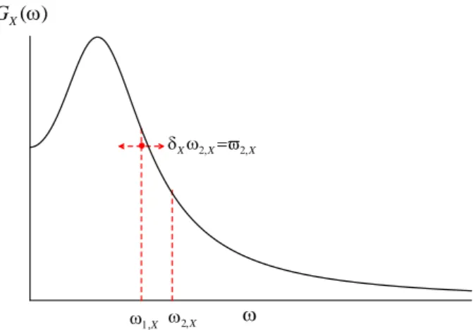
where _{1, X} is the frequency at the area centric of G_X , that indicates where the spectral density concentrates, and _{2, X} is the is the gyration radius of the area under the function G_X .

Figure 1. 4 Up-crossing (×) and down-crossing ( ) rate of the time axis of the random

process X t .

t X(t)

Another important parameter is the mean frequency, _X, which evaluates the variation in time of the mean up-crossing rate of the time axis (see Figure 1.4):

2,X

. 2

X (1.19)

The barycenter gyration radius _{2 , X} , or the measure of the dispersion around the frequency at the area centric of GX , is:

2 1, 2, 2, 2, 0, 0, 1 X X X X X X X (1.20) where 2 1, 0, 2, 1 X 0 1 X X X X (1.21)

is a non-dimensional parameter and it is called bandwidth

parameter, directly corresponding to coefficient of variation, that

measures the variation in the time of the narrowness of the stochastic process

X t

Figure 1. 5 Geometric representation of the SMs of the one-sided PSD function

X

G .

From the analysis of Figure 1.5 it is possible to have an immediate geometric representation of the SMs of the one-sided

PSD function G_X .

1.5 Distribution of extreme values for stationary

random process

The probability distribution of extrema of a random process is of particular interest in engineering design problems. In general, the extreme value of a stochastic process is a random variable.

Consider a zero-mean stationary Gaussian process

X t

X

t

represents the extreme value of

X t

max 0 max s t X t X s (1.22) G_X ( ) X X X X X

where the symbol denotes absolute value.

Figure 1. 6 Samples of the random process X t (dashed line), of the corresponding

absolute value X t (continuous line) and of the extreme value random

processX_max t (dash dot line).

In this way, the extreme value distribution for

X t

X

t

max

X

t

max , Pr max Pr : 0

X t

L u t X t u X s u s t (1.23)

in which the notation on the final term means that the X s u

inequality holds for all the given s values. The PDF for the extreme value, of course, is simply the derivative

max max d , d X t X t p u L u t u (1.24)

and from this information one can also calculate the mean, variance, s,t

X(k)_{(s), |} X(k)_(s)|,

Xmax

Once the PDF of the random process

X

t

X

X

represents the probability p that the maximum of the process X t

is inferior or equal to

X

0,t

max , ; Pr max( ) ,

X t t

F X _p t X t X _p p. (1.25)

The previous equation is a non-linear differential equation that can be alternatively solved introducing the dimensionless quantity

,

t

p

,

X

t

p

probability p of the dimensionless random process

max

/

Y t

X

t

max , ; Pr max( ) ,

X X X X X

F t p t X t t p p. (1.27)

A lot of hypothesis for the evaluation of the peak factor have been done in the literature; in particular for narrow band process the peak factor is given as (Vanmarcke 1975):

1 2, 0, 1/ 2 1 2, 1.2 0, ( , ) 2ln ln 1 exp ln ln . X X X X X X t t t p p p (1.28)

Once the peak factor _X

t

,

p

X

Chapter

2

Models of the ground motion acceleration

process

2.1 Introduction

The first step in structural engineering deals with a proper definition of the structural model and loads. For earthquake-resistant design of structures, the earthquake-induced ground motion is generally represented in the form of a response spectrum of pseudo-acceleration or displacement. The spectrum used as input is usually obtained by scaling an elastic spectrum by factors that account for, amongst other phenomena, the influence of inelastic structural response (Chopra 1995). There are, however, situations in which the scaled response spectrum is not considered appropriate, and a fully dynamic analysis is required. These situations may include structures with configuration in plan or elevation that is highly irregular; structures for which higher modes are likely to be excited; structures with special devices to reduce the dynamic response; buildings designed for a high degree of ductility and so on. Faced with these special situations, the engineer will generally have to

appropriate linear or non-linear models for the structure and a suitable suite of accelerograms to represent the seismic excitation (Bommer and Acevedo 2004).

There are three basic options available to the engineer in terms of obtaining suitable accelerograms. The first approach requires the generation of synthetic accelerograms from seismological source models and accounting for path and site effects (Lam et al. 2000, Rezaeian and Der Kiureghian 2010). In general, there are actual difficulties in defining appropriate input parameters such as the source, path, and site characteristics. Moreover, to generate synthetic accelerograms there is a need for a definition of a specific earthquake scenario in terms of magnitude, rupture mechanism in addition to geological conditions and location of the site. Generally, most of these parameters are not often available, particularly when using seismic design codes. It follows that the main limit of this approach is that practitioners cannot always accurately characterize the seismological threat to generate appropriate synthetic signals.

The second approach adopts real accelerograms recorded during earthquakes (Iervolino et al. 2010, Katsanos et al. 2010). Real accelerograms contain a wealth of information about the nature of the ground shaking, carry all the ground-motion characteristics (amplitude, frequency, and energy content, duration and phase characteristics), and reflect all the factors that influence accelerograms (characteristics of the source, path, and site). Due to the increase of available strong ground motion acceleration records, using and scaling real recorded accelerograms becomes one of most referenced contemporary research issues in this field. Despite the continued growth of the global strong motion database, there are many combinations of earthquake parameters such as magnitude, rupture mechanism, source-to-site distance and site classification

that are not well represented. It follows that their manipulation is relatively simple but often confusing and it is difficult to obtain suitable records in some circumstances.

The third approach uses artificial spectrum-compatible accelerograms. Artificial accelerograms are generated to match a target elastic response spectrum by obtaining a Power Spectral

Density (PSD) function from the smoothed response spectrum, and

then to derive harmonic signals having random phase angles (Vanmarcke and Gaparini 1977, Kaul 1978, Pfaffinger 1983, Preumont 1984, Cacciola et al. 2004). The attraction of these approaches is obvious because it is possible to obtain acceleration time-series that are almost completely compatible with the elastic design spectrum, which in some cases will be the only information available to the design engineer regarding the nature of the ground motions to be considered.

The simulation of artificial accelerograms is usually based upon a stationary stochastic zero-mean Gaussian process assumption; the stationary non-white models were suggested first by Kanai (1957), Tajimi (1960), Housner and Jennings (1964). These models, which account for site properties and for the dominant frequency in ground motion, fail to reproduce the typical characteristics of the real earthquakes: stationary artificial accelerograms generally have an excessive number of cycles of strong motion and consequently they possess unreasonably high energy content (Wang et al. 2005). Furthermore, the stationary model suffers the major drawback of neglecting the changes in amplitude and frequency content.

In order to overcome this drawback the so-called

quasi-stationary (or uniformly modulated non-quasi-stationary) random

1969, Hsu and Bernard 1978, Iwan and Hou 1989). These processes are constructed as the product of a stationary zero-mean Gaussian random process by a deterministic function of time; for this reason they are also called separable non-stationary stochastic processes.

Furthermore, a time-varying frequency content is observed in actual accelerogram records. This non-stationary frequency is prevalently due to different arrival times of the primary, secondary and surface waves that propagate at different velocities through the earth crust. Moreover, it has been shown that the non-stationarity in frequency content can have significant effects on the response of structures (see e.g. Saragoni and Hart 1973, Yeh and Wen 1990). The stochastic processes involving both the amplitude and the frequency changes are referred in literature as fully non-stationary random processes. The spectral characterization of the fully non-stationary processes is usually performed by introducing the

Evolutionary Power Spectral Density (EPSD) function (Priestley

1965). On the contrary of the stationary case, the EPSD function cannot be defined univocally. Then, several models have been proposed in literature. In particular Preumont (1985) derived the

EPSD function by imposing to the non-stationary model the equality

of the average energy for each frequency with respect the stationary case. Saragoni and Hart (1973) proposed a fully non-stationary model by juxtaposing time segments of gamma-functions modulated filtered zero-mean Gaussian white noises; Spanos and Solomos (1983) proposed a non-separable model introducing a particular

EPSD function; Yeh and Wen (1990) and Fan and Ahmadi (1990)

proposed a generalization of the Kanai-Tajimi model; Conte and Peng (1997) defined the ground motion acceleration as the sum of a finite number of pairwise independent uniformly modulated

zero-mean Gaussian stochastic process, the so-called sigma-oscillatory processes.

Another powerful strategy to analyse the evolutionary frequency content is based on the wavelet analysis (Spanos and Failla 2004, Spanos et al. 2005, Mallat 2009). Wavelet analysis is well suited to identify and preserve non-stationarity because the wavelet basis consist of compact functions of varying lengths. Each wavelet function corresponds to a finite portion of the time domain and has a different bandwidth in the frequency domain. The multiscale nature of wavelet analysis facilitates the simultaneous evaluation of non-stationarity in the time and frequency domains. Wavelet analysis has been performed by Suàrez and Montejo (2005) to simulate non-stationary ground motions. Moreover, several studies have been carried out to obtain fully non-stationary spectrum-compatible artificial accelerograms (Mukherjee and Gupta 2002, Giaralis and Spanos 2009 and Cecini and Palmeri 2015).

Alternatively, adaptive signal processing techniques can be adopted, such as the decomposition of the signal on a Gaussian chirplet set of functions and the empirical mode decomposition (see Yin et al. 2002,Politis et al. 2006, Spanos et al. 2007).

After a deep analysis of real earthquakes, in order to understand their main characteristics, the principal purpose of this Chapter is to examine the different models of the ground motion acceleration process that have been proposed in literature, for both the mono-correlated and the multi-mono-correlated input process.

Furthermore, a procedure to generate artificial spectrum-compatible fully non-stationary accelerograms is proposed; the generation of fully non-stationary accelerograms is performed in three steps. In the first step the spectrum-compatible PSD function in

the spectrum-compatible EPSD function is obtained by an iterative procedure to improve the match with the target response spectrum starting from the stationary PSD function, once a time-frequency modulating function is chosen. In the third step the accelerograms are generated by the Shinozuka and Jan (1972) formula and deterministic analyses can be performed to evaluate the structural response.

2.2 Real earthquakes

Earthquakes are vibrations of the earth surface caused by sudden movements of the earth crust which consists of rock plates that float on the earth mantle. The ground motion is due to the rupture of the rock when the shear stress exceeds the strength of the rock and the energy is released in the form of seismic waves. Two of the most common parameters related to a seismic event are the earthquake

magnitude (M) and distance (R) (in km) of the rupture zone from the

site of interest.

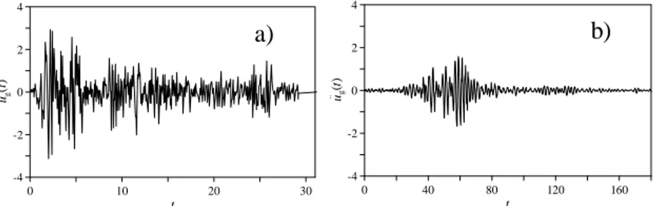
Figure 2. 1 a) El Centro NS recorded earthquake, 1940; b) Mexico City N90W recorded earthquake, 1985.

It is obvious that every accelerogram is sensitively different from the others, as shown in Figure 2.1, mainly due to the characteristics of the specific location of the propagation path of the seismic waves.

0 10 20 30 t -4 -2 0 2 4 u . . (tg ) 0 40 80 120 160 t -4 -2 0 2 4 u . . (tg ) a) b)

For engineering purposes, the ground motion caused by seismic waves is measured by accelerometers or accelerographs which record three components of the ground acceleration, two horizontal and one vertical. The earthquake accelerograms by themselves provide general information among which the Peak Ground

Acceleration (PGA) and the total seismic duration t_d. The PGA is the most simple and widely used intensity index for seismic structural analysis purposes. It is also adopted in many structural design codes or provisions worldwide. Although PGA is an important intensity index, its scope of application is limited because a single measure is unable to fully describe the complex earthquake characteristics. For further information an elaboration of the accelerograms is necessary. The results of this elaboration are characteristic parameters, either in the time or in the frequency domain. Some parameters in the time domain are the ARIAS

intensity, the HUSID diagram, the Strong Motion Duration (SMD).

On the other hand, some parameters in the frequency domain are the spectral intensities and the Fourier spectra. The ARIAS intensity is a measure of the strength of a ground motion and it is usually defined by the following relationship:

2 A g 0 ( ) d , 2 g d t I u t t (2.1)

where g is the acceleration due to gravity and u t_g( ) is the recorded accelerogram. The HUSID diagram, H t( ), is the time history of the seismic energy content scaled to the total energy content and it is defined by the following relation:

2 g 0 2 g 0 ( ) d ( ) . ( ) d d t t u H t u t t (2.2)

By means of the HUSID diagram it is possible to define the SMD, s

T, as the time elapsed between the 5% and 95% of the HUSID diagram defined by the following relation:

0.95 0.05

s

T t t (2.3)

where t_0.95 is the time elapsed at the 95% of the HUSID diagram and

0.05

t the time elapsed at the 5% of the HUSID diagram.

Figure 2. 2 Husid Function and definition of the SMD: a) El Centro NS, 1940; b) Mexico city N90W, 1985.

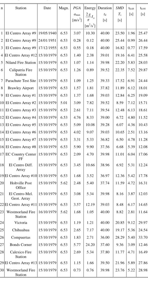
Table 2. I Characteristics of real earthquakes.

Site Year PGA

amax [m/s2] Arias Intensity A I [m/s] Duration td [s] SMD Ts [s] t0.05 [s] t0.95 [s] El Centro NS 1940 3.13 1.78 31.16 24.20 1.63 25.83 Mexico City 1985 1.68 2.45 180.08 40.71 39.68 80.38

In order to understand the main characteristics of real earthquakes, a statistical study has been performed, by selecting a

0 10 20 30 t 0 0.2 0.4 0.6 0.8 1 H (t ) 0 40 80 120 160 t 0 0.2 0.4 0.6 0.8 1 H (t ) a) b)

set of recorded accelerograms and analysing the time-frequency behaviour.

The chosen database is the “PEER: Pacific Earthquake Engineering Research Center: NGA Database”; 30 recorded accelerograms have been selected to perform the statistical analysis. In particular, all of them are time histories of seismic events that happened in the Imperial Valley (California) (see Figures 2.3, 2.4).

Figure 2. 3 Some of the seismic events in Imperial Valley.

In the following Figures all the ground motion time history are shown.

Figure 2.4 a) Registration of earthquakes in the Imperial Valley, California. 0 10 20 30 40 t -0.4 -0.2 0 0.2 0.4 u .. g (t )/ g (1) 0 10 20 30 40 t -0.04 -0.02 0 0.02 0.04 u .. g (t )/ g (2) 0 10 20 30 40 t -0.08 -0.04 0 0.04 0.08 u .. g (t )/ g (3) 0 10 20 30 40 t -0.2 -0.1 0 0.1 0.2 u .. g (t )/ g (4) 0 10 20 30 40 t -0.12 -0.08 -0.04 0 0.04 0.08 0.12 u .. g (t )/ g (5) 0 10 20 30 40 t -0.1 -0.05 0 0.05 0.1 0.15 u .. g (t )/ g (6) 0 10 20 30 40 t -0.12 -0.08 -0.04 0 0.04 0.08 0.12 u .. g (t )/ g (7) 0 10 20 30 40 t -0.2 -0.1 0 0.1 0.2 u .. g (t )/ g (8)

0 10 20 30 40 t -0.2 -0.1 0 0.1 0.2 u .. g (t )/ g (9) 0 10 20 30 40 t -0.4 -0.2 0 0.2 0.4 u .. g (t )/ g (10) 0 10 20 30 40 t -0.4 -0.2 0 0.2 0.4 u .. g (t )/ g (11) 0 10 20 30 40 t -0.4 -0.2 0 0.2 0.4 0.6 u .. g (t )/ g (12) 0 10 20 30 40 t -0.6 -0.4 -0.2 0 0.2 0.4 u .. g (t )/ g (13) 0 10 20 30 40 t -0.6 -0.4 -0.2 0 0.2 0.4 u .. g (t )/ g (14) 0 10 20 30 t -0.4 -0.2 0 0.2 0.4 u .. g (t )/ g (15) 0 10 20 30 t -0.4 -0.2 0 0.2 0.4 0.6 u .. g (t )/ g (16)

Figure 2.4 c) Registration of earthquakes in the Imperial Valley, California.

0 10 20 30 40 t -0.2 -0.1 0 0.1 0.2 0.3 u .. g (t )/ g (17) 0 10 20 30 40 t -0.4 -0.2 0 0.2 0.4 u .. g (t )/ g (18) 0 10 20 30 t -0.2 -0.1 0 0.1 0.2 u .. g (t )/ g (19) 0 10 20 30 t -0.3 -0.2 -0.1 0 0.1 0.2 0.3 u .. g (t )/ g (20) 0 10 20 30 40 t -0.4 -0.2 0 0.2 0.4 u .. g (t )/ g (21) 0 10 20 30 40 t -0.4 -0.2 0 0.2 0.4 u .. g (t )/ g (22) 0 10 20 30 40 t -0.1 0 0.1 0.2 u .. g (t )/ g (23) 0 10 20 30 40 t -0.15 -0.1 -0.05 0 0.05 0.1 u .. g (t )/ g (24)

Figure 2. 4 d) Registration of earthquakes in the Imperial Valley, California.

For each of the recorded accelerograms the mean frequency has been evaluated, as shown in Figure 2.5.

0 10 20 30 40 t -0.3 -0.2 -0.1 0 0.1 0.2 u .. g (t )/ g (25) 0 10 20 30 t -0.2 -0.1 0 0.1 0.2 u .. g (t )/ g (26) 0 10 20 30 40 t -0.8 -0.4 0 0.4 0.8 u .. g (t )/ g (27) 0 10 20 30 40 t -0.4 -0.2 0 0.2 0.4 u .. g (t )/ g (28) 0 10 20 30 40 t -0.15 -0.1 -0.05 0 0.05 0.1 0.15 u .. g (t )/ g (29) 0 10 20 30 40 t -0.08 -0.04 0 0.04 0.08 u .. g (t )/ g (30)

Figure 2. 5 Mean frequency of the i-th accelerogram.

Figure 2. 6 Arithmetic average of the up-crossing time axis rate, g

U t [s

-1

], of the 30 accelerograms recorded in the Imperial Valley (California-USA).

Then, in order to perform a statistical analysis the average of the mean frequency

g

U t (see Figure 2.6) has been determined. This figure shows both the time-varying amplitude and frequency content of recorded accelerogram.

In Table 2.II the main characteristics of these 30 accelerograms are reported. Namely: the station name, the date of the recorded event, the magnitude, the PGA, the energy, the strong motion

duration as well as t_0.05and t_0.95. From the analysis of these accelerograms the following average parameters are obtained:

14.40 s

T

t

5.04 s

t

19.44 s

Table 2. II Main characteristics of the accelerograms recorded in the Imperial Valley (California-USA)

n Station Date Magn. PGA

amax [m/s2] Energy 2 A g I [m2/s3] Duration td [s] SMD Ts [s] t0.05 [s] t0.95 [s] 1 El Centro Array #9 19/05/1940 6.53 3.07 10.30 40.00 23.50 1.96 25.47 2 El Centro Array #9 24/01/1951 6.53 0.28 0.12 40.00 25.44 0.99 26.44 3 El Centro Array #9 17/12/1955 6.53 0.55 0.18 40.00 16.82 0.77 17.59 4 El Centro Array #12 15/10/1979 6.53 1.40 2.38 39.01 19.16 6.41 25.58

5 Niland Fire Station 15/10/1979 6.53 1.07 1.14 39.98 22.20 5.83 28.03

6 Calipatria Fire

Station

15/10/1979 6.53 1.26 0.89 39.52 22.35 7.52 29.87

7 Parachute Test Site 15/10/1979 6.53 1.09 1.25 39.33 17.52 6.91 24.44

8 Brawley Airport 15/10/1979 6.53 1.57 1.81 37.82 11.89 6.12 18.01 9 El Centro Array #1 15/10/1979 6.53 1.37 1.68 39.03 12.84 6.25 19.09 10 El Centro Array #2 15/10/1979 5.01 3.09 7.82 39.52 8.59 7.12 15.71 11 El Centro Array #3 15/10/1979 6.53 2.61 7.11 39.54 12.48 6.13 18.61 12 El Centro Array #4 15/10/1979 6.53 4.76 8.33 39.00 6.72 4.80 11.52 13 El Centro Array #5 15/10/1979 6.53 5.09 10.08 39.28 6.07 4.36 10.43 14 El Centro Array #6 15/10/1979 6.53 4.02 9.07 39.03 10.65 2.51 13.16 15 El Centro Array #7 15/10/1979 6.53 3.31 5.33 36.82 6.50 4.78 11.28 16 El Centro Array #8 15/10/1979 6.53 5.90 9.90 37.56 6.68 5.39 12.08 17 EC Country Center FF 15/10/1979 6.53 2.09 4.70 39.98 11.01 6.04 17.06 18 El Centro Diff. Array 15/10/1979 6.53 3.45 10.66 38.96 6.92 5.31 12.24 19 El Centro Array #10 15/10/1979 6.53 1.68 3.52 36.97 12.36 5.42 17.78 20 Holtville Post Office 15/10/1979 5.62 2.48 5.40 37.74 11.59 4.72 16.31 21 El Centro-Mel. Geot. Array 15/10/1979 6.53 3.08 5.34 39.98 8.16 3.87 12.03 22 El Centro Array #11 15/10/1979 6.53 3.57 12.19 39.03 8.48 6.17 14.65 23 Westmorland Fire Station 16/10/1979 5.62 1.68 1.05 40.00 8.82 2.81 11.64 24 Victoria 15/10/1979 6.53 1.19 1.21 40.00 20.85 9.12 29.97 25 Chihuahua 15/10/1979 6.53 2.65 7.17 40.00 19.17 5.36 24.54 26 Compuertas 15/10/1979 6.53 1.83 2.71 36.00 28.29 5.40 33.70 27 Bonds Corner 15/10/1979 6.53 5.77 24.20 37.60 9.36 3.09 12.46 28 Calexico Fire Station 15/10/1979 6.53 2.69 5.34 37.80 11.77 4.71 16.49 29 El Centro Array #13 15/10/1979 6.53 1.15 1.66 39.50 21.96 5.89 27.86

2.3 The evolutionary process model

In this section the characterization of the non-stationary model of the ground motion acceleration process will be done following the Priestley (1965, 1967) evolutionary process model. Firstly the spectral description of the non-stationary stochastic process is done; then four models of modulating functions, for both the quasi-stationary and fully non-quasi-stationary process, amongst the most common present in literature, will be presented.

2.3.1 Definition of the non-stationary stochastic input

Fourier-Stieltjes integral (Priestley 1965, Priestley 1967):

( )t exp(i t a) ( , ) dt N

F

where i 1 is the imaginary unit, a( , )t is a slowly varying complex deterministic time-frequency modulating function, which has to satisfy the condition: a( , )t a ( , )t , where the asterisk denotes the complex conjugate; N( ) is a process with orthogonal increments, so that its increments d (N ₁) and d (N ₂) at any two distinct points ₁ and ₂ are uncorrelated random variables, satisfying the conditions:

*

1 2 1 2 0 1 1 2

In Eq. (2.5) the symbol E means stochastic average and is the Dirac delta defined as:

0 0 0 0, ; , ; t t t t t t (2.6) 0( )

S is the PSD function of the so-called “embedded” stationary counterpart process (Michaelov et al. 1999a). It is a real and symmetric function: S₀( ) S₀( ).

It has to be emphasized that the stochastic process F( )t is also termed oscillatory process since it possesses evolutionary spectrum belonging to the family of the oscillatory functions _q defined as

exp( ) ( , )

q i t

a

F

F

F

which is a real symmetric function given as:

* 1 2 1 2 1 2 0 1 2 1 2 , exp i ( , ) ( , ) ( ) d exp i ( , , ) d . FF FF R t t t t a t a t S t t S t t (2.7)

In the evolutionary process analysis (Priestley 1999), the function: 2 0 ( , ) ( , ) ( ) FF S t a t S (2.8)

is called EPSD function of the non-stationary process F( )t . In the previous equation the symbol denotes the modulus of the function in brackets. The processes characterized by the EPSD function

( , ) FF

S t , are called fully non-stationary random process, since both time and frequency content change. If the modulating function is a real time dependent function, a( , )t a t( ), the non-stationary process is called quasi-stationary (or uniformly modulated) random process.

In the stochastic analysis the one-sided EPSD function is generally used; the latter, in the Priestley representation, can be suitably defined by the following relationships:

* 1 2 0 1 2 1 2 ( , ) ( , ) ( ) 2 ( , , ) , 0; ( , , ) 0 , 0, FF FF a t a t G S t t G t t (2.9) where G₀( )

G

( )

2 ( ), 0;

S

G

( )

0,

0

one-sided PSD function of the stationary counterpart of input process F t( ).

2.3.2 Models of the non-stationary random process

Among the modulating functions that are herein considered, the simplest one, a t₁( ), that defines an uniformly modulated random process, has been proposed by Hsu and Bernard (1978):

1

( )

exp

a t

t

t

1 1

exp 1 .

The constant ₁ normalizes the exponential modulating function so that the maximum of the real function a t₁( ) is unity.

Figure 2. 7 Hsu and Bernard (1978) modulating function, 1 1/ 6.

2) Normalized exponential type II modulating function

Another time modulating function, among the most used in literature, a t₂( ) has been proposed by Shinozuka and Sato (1967):

2( ) 2 exp 2 exp 3 .

a t t t (2.12)

The constant ₂ normalizes the exponential modulating function so that the maximum of the real function a t₂( ) is unity; it can be evaluated as: 2 3 3 2 3 2 3 2 2 exp ln . (2.13) 0 10 20 30 t 0 0.2 0.4 0.6 0.8 1 1.2 a1 (t )

Figure 2. 8 Shinozuka and Sato (1967) modulating function, 2 0.045 , 3 0.05 .

3) Normalized Jennings et al. type modulating function

This modulating real function initially increases parabolically (up to time t₁), remains constant between times t₁ and t₂, and then decreases exponentially. This was proposed by Amin and Ang (1968) and by Jennings et al. (1969). The normalized to unity expression can be written as:

3 2 1 1 2 4 2 2 1 ( ) (0, ) ( , ) exp ( ) 2 t a t t t t t t t t t (2.14)

where ( , )t t_{i j} and ( )t are the window and the unit-step functions defined as: 0 0 0 1, ; 0, ; ( , ) ( ) 0, , ; 1, . i j i j i j t t t t t t t t t t t t t t t (2.15) 0 10 20 30 t 0 0.2 0.4 0.6 0.8 1 1.2 a2 (t )

Figure 2. 9 Jennings et al. (1969) modulating function, t1 4 ,s t2 14 ,s 4 0.3.

4) Normalized Spanos and Solomos model of the fully

non-stationary process

In order to take into account the main features of seismic ground motion, that is the “build-up” and the “die off” segments as well as a decreasing dominant frequency, Spanos and Solomos (1983) proposed the following time-frequency modulating function,

4( )

a t :

4( ) 4 exp 5

a t t t (2.16)

with the parameter ₄ that normalizes the time-frequency modulating function so that the maximum of the real function

4( , ) a t is unity. 0 10 20 30 t 0 0.2 0.4 0.6 0.8 1 1.2 a3 (t )

Figure 2. 10 Spanos and Solomos (1983) modulating function, 4 max 1 2 , 5 a 2 5 2 max 1 0.15 , 6.007. 2 500 a

2.4 Wavelet analysis

In order to identify and preserve the non-stationarity of the real earthquakes, a powerful tool is represented by the wavelet analysis. In fact, the use of wavelets permits a joint time–frequency signal representation.

The wavelet transform gives a time-frequency representation of a signal F t( ), belonging to the family of finite energy functions:

2

( ) d

E F t t (2.17)

by a double series of basis functions called “wavelets” _{u s,} t . Each wavelet is a local function of time, it possesses a certain frequency content and it is generated by scaling, by the parameter s

(controlling the frequency distribution), and shifting, by the parameter

u

The continuous wavelet transform of the signal F t( ), at scale s and position u is given by:

*

, , d

u s u s

a F t t t (2.18)

where the asterisk denotes the complex conjugate and

, 1 . u s t u s s (2.19)

The signal F t( ) will be obtained from the inverse continuous wavelet transform: , , 2 0 1 1 d d u s u s F t a t s u C s (2.20)

in which C is a normalizing constant.

Unfortunately the wavelet is a decaying function, so it is impossible to localize it in time. However families of wavelets can be conveniently generated in a way to form an orthogonal basis, so that the wavelet transform is bijective, giving a unique representation. Among the proposed models, Newland (1994) introduced a class of harmonic wavelets, having a box-shaped band limited spectrum. Later, the filtered harmonic wavelet scheme was presented by the same author (Newland 1999) incorporating a Hanning window function in the frequency domain to improve the time localization capabilities of the harmonic wavelet transform in the wavelet mean square map for a given frequency resolution

(Newland 1999, Spanos et al. 2005). In this case, the wavelet function of scale (m, n) and position (k) in the frequency domain takes the form:

, , 1 2 1 cos , 2 ; 0, elsewhere. m n k m m n n m n m (2.21)

By applying the inverse Fourier transform it is possible to obtain the complex-valued time domain counterpart, having magnitude

, , 2 2 sin 1 m n k k t n m n m t k k t t n m n m n m (2.22) and phase: , , . m n k k t t m n n m (2.23)

The harmonic wavelet transform of the signal F t( ) will be given by

*

, , , , d

m n k m n k

a n m F t t t (2.24)

and, in order to perform a time-frequency analysis, the wavelet spectrogram can be derived

2 , ,

, _{m n k} .

SP t a (2.25)

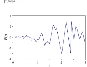
Figure 2. 11 Approximation of the first seconds of the El Centro NS recorded earthquake, 1940 (black line) with the wavelet decomposition (blue dashed line).

Figure 2.11 shows an example of approximation of a given signal

( )

F t through the wavelets analysis.

2.5 Adaptive chirplet decomposition

In the framework of fully non-stationary processes, it is possible to use the adaptive chirplet decomposition in order to represent the forcing input. In particular the Gaussian chirplets are able to catch the modulation in frequency and in time of the signal and are suited for the decomposition of highly non-stationary signals.

For a given signal F t( ), Mallat and Zhang (1993) and Qian and Chen (1995), developed independently the Matching Pursuit (MP) algorithm that permits its decomposition if the following relationship is satisfied: 2 ( ) d E F t t (2.26) 0 1 2 3 t -4 -2 0 2 4 F (t )

where E is the total energy of the signal. The MP provides the following decomposition of the signal:

( ) _{k k} k

F t A h t (2.27)

where

h t

2 4 2 exp / 2 exp / 2 exp k k k k k k k k a h t a t t i t t i t t (2.28)

with _k that is a scaling factor, t_k and _k that shift in time and in frequency, respectively, the chirplet and the chirprate _k that leads to a linear frequency modulation (Mann and Haykin 1995) .

The coefficients A_k are obtained such as the mean square error between the signal and its approximation is minimum. This leads to the solution of the optimization problem:

2 2 2 max , max d . k k k k k k k h h A F t h t F t h t t (2.29)

First, the original signal

F t

F t

k

0

all the functions of the dictionary and the coefficient A₀ is determined from Eq.(2.29). Then, the residual

F

t

1

.

k k k k

This procedure, described above for the original signal, is repeated for the residual iteratively, and the algorithm terminates when the energy of the residual reaches a desired predefined level that obviously characterizes the quality of the approximation (Spanos et al. 2007).

Figure 2. 12 Approximation of the firts seconds of the El Centro NS recorded earthquake, 1940 (black line) with adaptive chirplet decomposition (blue dashed line).

Applying the Wigner-Ville distribution, the adaptive spectrogram can be derived: 2 2 2 0 , 2 exp / K k k k k k k k k AS t A t t t t (2.31) and then it is possible to generate the artificial seismic waves (Yang 1986) 0 1 ( ) , cos n r r k k k k k F t AS t G t (2.32) 0 1 2 3 t -4 -2 0 2 4 F (t )

where is the frequency increment, _k is the discrete frequency,

r

k is the random phase with uniform distribution between

0

2

G

2.6 Fully non-stationary spectrum compatible

seismic waves

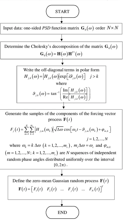
2.6.1 Simulation of the random process samples

The problem of simulating spectrum-compatible earthquake accelerograms is addressed on a probabilistic basis under the assumption that an earthquake accelerogram is considered as a sample of a random process. The samples must satisfy two exigences:

- they have to be random;

- they must describe the probabilistic characteristics of the corresponding stochastic process.

Figure 2. 13 Approximation of the one-sided PSD function for the generation of samples of a stationary Gaussian random process.

G_F ( )

k

2 GF( k)

A zero-mean stationary Gaussian random process F t is completely defined by the autocorrelation function R_F or by the corresponding one-sided PSD function G_F ; in order to apply the simulation technique is firstly necessary to sample this one, as shown in Figure 2.13.

It is necessary to define a cut off frequency such that:

2 2

0

F F F

G (2.33)

where G_F 0if ; for the ground motion acceleration process G_F 0 if

100 rad/s

Once the cut off frequency has been chosen, the interval 0, is divided in m_c interval of amplitude /m_c, with the central point _k

k

,1,2,. ,

m

k GF k . So the r-th sample

F

t

where is the frequency increment, _kr is the random phase with uniform distribution between

0

2

When the process is a uniformly-modulated or fully non-stationary random process, with modulating function, respectively,

a t

a

,

t

1 1 ( ) 2 sin ( ) , 2 sin c c m r r F k k m r r F k k F t a t G k k t + F t a k t G k k t + (2.35)

Notice that the implementation of Eqs.(2.35) leads to a greater computational cost then (2.34); this is mainly due to the introduction of the modulating functions

a t

a

,

t

2.6.2 Stationary spectrum-compatible accelerograms

Several methods for generating a spectrum-consistent PSD function are available in the literature (Vanmarcke and Gaparini 1977, Kaul 1978, Pfaffinger 1983, Preumont 1984, Cacciola et al. 2004).

Here the method proposed by Cacciola et al. (2004) is briefly described. This method considers the ground-acceleration as a sample of a zero-mean stationary Gaussian process. It approximates the pseudo-acceleration response spectrum as the 50% fractile of the peak maxima distribution of the response process of a Single Degree of Freedom (SDOF) oscillator subjected to the earthquake

acceleration zero-mean process,

U t

2

0 0 0

( ) 2 ( ) ( ) _g .

U t U t U t U t (2.36)

Consequently the following very handy recursive expression of the one-sided PSD function of the earthquake acceleration zero-mean process,

U t

pseudo-acceleration response spectrum, is obtained (Cacciola et al. 2004):

g g g ST 2 ₁ pa 0 ST 0 ST U 2 1 0 1 0 ( ) 0, 0 ; ( , ) 4 ( ) ( ) , ; 4 ( , ) k k i U k k k j i k f U j k k U k G S G G (2.37)

where the apex ST evidences that the one-sided PSD function is evaluated in the hypothesis of stationary random processes,

1(rad s)

i (Cacciola et al. 2004) and f are chosen as bounds of the existence domain of the one-sided PSD function

g

ST

( ) U

G . In Eq.(2.37)

S

(

, )