Use of advanced mass spectrometry technologies for the analysis of high complex samples

Università degli Studi di Messina

Dipartimento di Scienze chimiche, biologiche, farmaceutiche e ambientali

“Doctor of Philosophy in “Chemical Science”

“

Use of Advanced Mass Spectrometry Technologies for the

Analysis of High Complex Samples

Ph.D. Thesis of: Marco Piparo

Supervisor: Prof. Luigi Mondello Coordinator: Prof. Sebastiano Campagna

Index

TABLE OF CONTENTS

Scope of the research work 2

Chapter 1. Mass spectrometry: Fundamental and Instrumentation

1.0. Introduction 4

1.1. Brief history and basic principles of mass spectrometry 5

1.2. Mass spectrometers 8

1.2.1. Mass spectrum 10

1.3. Mass resolution and mass accuracy 12

1.3.1. Resolution and resolving power 12

1.3.2. Mass accuracy 14

1.3.2.1. Exact mass and role of the electron mass 15 1.3.2.2. Mass accuracy and determination

of molecular formulas 16

1.3.2.3. High mass molecules influence of resolution

on isotopic pattern and mass accuracy 17

1.4. Instrumentation 18

1.4.1. Ions sources 20

1.4.1.1. Electron ionization (EI) ion sources 21

1.4.1.2. Sample introduction 23

1.4.1.3. Databases of EI mass spectra 24

1.4.2. Mass analyzers 25

1.4.2.1 Quadrupole mass spectrometers 26 1.4.2.2 Time of flight spectrometers 29

Index

2

1.4.2.2.2. Orthogonal acceleration 34 1.4.2.3. Ion mobility spectrometers 34 1.4.2.3.1 Collision cross section 37

1.4.2.3.2 Resolution 38

1.4.3. Tandem mass spectrometry 40

References 43

Chapter 2. Comprehensive two-dimensional gas chromatography fundamentals and theoretical/practical considerations

2.0. Introduction 48

2.1. Theory of gas chromatography 50

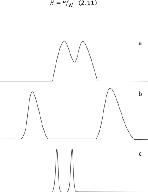
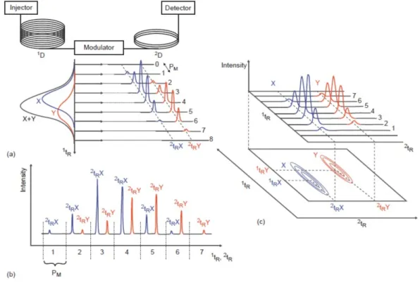
2.2. Why comprehensive two-dimensional gas chromatography 64

2.3. The concept of multidimensionality 67

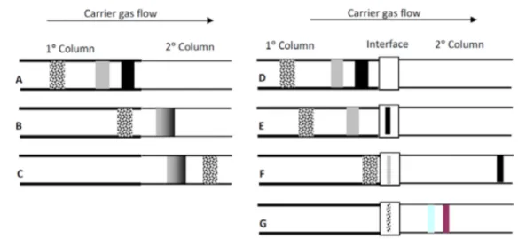
2.3.1. From MDGC to GC×GC 69 2.4. GC×GC: basic instrumentation 75 2.4.1. Columns combination 75 2.4.2. Transfer devices 79 2.4.3. Detectors 80 2.4.4. Modulators 83 2.4.4.1. Cryogenic interfaces 84 2.4.4.2. Valve-based devices 89 References 99

Index

3

Chapter 3. Research in the field of comprehensive two-dimensional gas chromatography coupled to various forms of mass spectrometry

3.0. Multidimensional gas chromatographic techniques applied to the analysis of lipids from wild-caught and farmed marine species

3.1. Introduction 106

3.2. Experimental 108

3.2.1. Samples and sample preparation 108

3.2.2. GC-FID analysis 109

3.2.3. GC×GC–MS analysis 109

3.3. Results and discussion 110

3.3.1 Fatty acid composition and distribution 110

3.3.2. GC×GC distribution pattern 115

3.4. Conclusion 118

References 122

Chapter 4. Fast gas chromatography

4.0. Introduction 126

4.1. Routes towards faster separation 127

4.2. Selecting the optimal method for minimizing

time of operation 129 4.3. Definitions in fast GC 143 4.4. Instrumentation 144 4.4.1. Carrier gas 144 4.4.2. Pressure regulators 145 4.4.3. Injection systems 145 4.4.4. Columns 147

Index

Chapter 5. Cryogenic modulation fast comprehensive gas

chromatography-mass spectrometry by using a 10m micro-bore column combination: concept, method optimization and application

5.0. Introduction 156

5.1. Experimental 158

5.1.1. Standard compounds and sample 158

5.1.2. Instrumentation 158

5.2. Results and discussion 161

5.3. Conclusions 169

References 170

Chapter 6. Ultra-High Pressure Liquid Chromatography Coupled with Ion Mobility Mass Spectrometer

6.0. Introduction to ultra-high pressure liquid chromatography 174

6.1. UHPLC system requirements 177

6.2. Moving from a HPLC method to an UHPLC 179 6.3. Introduction to ion mobility spectrometry 181 6.4. A measurement by ion mobility spectrometry 184 6.5. The mobility of ions in an electric field through gases 184

6.6. Instrumentation 187

6.6.1. Ion source 189

6.6.2. IMS entrance section 189

Index

5

6.6.4. IMS exit section 192

6.7. Methods of ion mobility spectrometry 194

6.7.1. Field asymmetric IMS, differential mobility spectrometry,

ion drift spectrometry 194

6.7.2. Travelling wave methods of IMS 195

6.7.3 Atmospheric pressure drift tube ion mobility–mass

spectrometry 198

References 202

Chapter 7. Discovering biological metabolite isomers from different mammalian species with liquid chromatography drift tube-ion mobility mass spectrometry

7.0. Introduction 210

7.1. Experimental 211

7.1.1. Samples and sample preparation 211

7.1.2. UHPLC-IM-Q-ToF analysis 212

7.2. Results and discussions 213

Abstract

2

Scope of the research work

My research work, during the Ph.D. course, has been focused mainly on the use different mass spectrometry techniques for the analysis of complex sample. Much of the experimentation has been performed in the field of gas chromatography, even though liquid chromatography has also been exploited. The techniques used have been: single quadrupole mass spectrometry tandem with comprehensive gas chromatography (GC×GC-MS), single quadrupole mass spectrometry tandem with fast comprehensive gas chromatography, and quadrupole time of flight tandem with ion mobility (IM-Q-ToF). The use of such powerful analytical instrumentation, enabled the attainment of detailed information of sample, and in particular related to food safety. Comprehensive 2D GC is a relatively new technique, developed in 1991 and can be considered, without a doubt, at the same level of the OTC, in terms of the revolutionary impact that it has had on the GC field.

With regards to loop-type cryogenic modulation, I have been involved in food-sample applications (mussels, claim and fish) and in the optimization and development studies. In the latter case the use of micro bore columns in both dimensions is emphasized.

Regarding the ion mobility Q-ToF I have involved in the separation of isomers in different type of milk and in the calculation of collision cross section value improve lipid identification.

Mass Spectrometry: Fundamental and Instrumentation

3

Chapter 1

Mass spectrometry: Fundamental and

Instrumentation

Mass Spectrometry: Fundamental and Instrumentation

4

1.0 Introduction

For over 100 years, mass spectrometry has played a crucial role in a variety of scientific disciplines. With a small beginning in the late nineteenth century as a tool to detect cathode rays, mass spectrometry currently has assumed a major role in identification of proteins in biological experiments, with the aim of unravelling their functional role and detecting biomarkers of a specific disease. Mass spectrometry has become an integral part of proteomics and the drug development process. Several diverse fields, such as physics, chemistry, medicinal chemistry, pharmaceutical science, nuclear science, food science, petroleum industry, forensic science, and environmental science, have benefited from this highly sensitive and specific instrumental technique. Mass spectrometry’s characteristics have raised it to an outstanding position among analytical methods: unequalled sensitivity, detection limits, speed and diversity of its applications. In analytical chemistry, the most recent applications are mostly oriented towards biochemical problems, such as proteome, metabolome, high throughput in drug discovery and metabolism, and so on. Other analytical applications are routinely applied in pollution control, food control, forensic science, natural products or process monitoring. Regardless of the analytical purpose, mass spectrometry aims to provide structural information of a compound for an unambiguous identification. The fundamental requisite for a successful mass spectrometric experiment is the generation of stable ions of the molecules of interest capable to “survive” along their path inside the mass spectrometer and, thus, to become detectable. In this respect, the molecule has to be firstly transferred from its existing physical state (either liquid or solid) to the gas phase into the vacuum of an ion source block, and afterwards it has to acquire one or several charges to be

Mass Spectrometry: Fundamental and Instrumentation

5

separated and detected into a mass analyser

From the 1950s to present, mass spectrometry has evolved tremendously in terms of developing of new and/or improving existing methods of ion sampling, generation and transfer into mass analyzers, as well as data recording and generation of mass spectra [1]. In particular, in the decade between 1995 and 2005 this progress has led to the advent of entirely new instruments. New atmospheric pressure sources were developed [2-5], existing analysers were perfected and new hybrid instruments were realized by new combinations of analysers.

There is no one-and-only approach to the wide field of mass spectrometry. Is necessary to learn about the ways of sample introduction, generation of ions, their mass analysis and their detection as well as about registration and presentation of mass spectra and each of these parts play a key role in the importance of successful application of mass spectrometry (Figure 1.1)

1.1. Brief history and basic principles of mass spectrometry

In 1897, Joseph John Thomson, a physicist, demonstrated the existence of the electron and measured its mass-to-charge (m/z) [6]. He later applied similar methods to the analysis of positive ions with positive ray parabolas [7]. In 1919, Aston, a student of Thomson, refined such an instrumentation by improving the use of electric and magnetic fields to focus ions on a photographic plate used as detector (focusing speed) [8]. Aston himself called that device mass spectrograph. After, Dempster constructed an instrument with a deflecting magnetic field angled at 180°. In order to detect different masses, it could have a variable magnetic field, and after focus them onto an electric point detector [9]. Later, the term mass spectrometer was coined for those type of instruments using a scanning magnetic field [10]. Aston and

Mass Spectrometry: Fundamental and Instrumentation

6

Dempster, along with the aforementioned Thomson, can therefore be considered as the pioneers of mass spectrometry.

Figure 1.1. The main domains of mass spectrometry

Three basic steps are involved in mass spectrometry analysis (Figure 1.2): 1. The first step is ionization that converts analyte molecules or atoms into gas-phase ionic species. This step requires the removal or addition of an electron or proton(s). The excess energy transferred during an ionization event may break the molecule into characteristic fragments.

Mass Spectrometry: Fundamental and Instrumentation

7

Figure 1.2. Basic concept of mass spectrometry analysis.

2. The next step is the separation and mass analysis of the molecular ions and their charged fragments on the basis of their m/z (mass-to-charge) ratios. Ion separation is effected by electric and/or magnetic fields. This former definition of mass spectrometry dates back to 1968 [11]

3. Finally, the ion current due to these mass-separated ions is measured, amplified, and displayed in the form of a mass spectrum.

The first two steps are carried out under high vacuum, which allows ions to move freely in space without colliding or interacting with other species. Collisions may lead to fragmentation of the molecular ions and may also produce a different species through ion–molecule reactions. These processes will reduce sensitivity, increase ambiguity in the measurement, and decrease resolution. In addition, the atmospheric background will introduce interference.

The analyte may be ionized thermally, by electric fields or by impacting energetic electrons, ions or photons. The energy deposited on the analyte during ionization processes can be varied, and this leads to classification of the various ionization techniques on the basis of their relative “softness” or “hardness” features. Another consideration is that ions can be mass separated

Mass Spectrometry: Fundamental and Instrumentation

8

in field-free regions (e.g., in time-of-flight analyzers). In such a case, the separation of ions within a given m/z range would be entirely governed by their masses, which will determine the time they spend into the drift region (a detailed discussion of the main mass analyzers will be presented in the next sections).

1.2. Mass spectrometers

A simplistic view of the essential components of a mass spectrometer is given in Figure 1.3. These components are:

1) An inlet system: transfers a sample into the ion source. An essential requirement is to maintain the integrity of the sample molecules during their transfer from atmospheric pressure to the ion-source vacuum.

2) An ion source: converts the neutral sample molecules into gas-phase ions. Several ionization techniques have been developed for this purpose.

Mass Spectrometry: Fundamental and Instrumentation

9

3) A mass analyser: separates and mass-analyzes the ionic species. Magnetic and/or electric fields are used in mass analyzers to control the motion of ions. A magnetic sector, quadrupole, time-of-flight, quadrupole ion trap, quadrupole linear ion trap, orbitrap, and Fourier transform ion cyclotron resonance instrument are the most common forms of mass analyzers currently in use.

4) A detector: measures and amplifies the ion current of mass-resolved ions. 5) A data system: records, processes, stores, and displays data in a form that human eye can easily recognize (computer screen or printer output).

6) A vacuum system: maintains a very low pressure in the mass spectrometer. The ion source region is usually maintained at a pressure of 10−4 to 10−8 torr; somewhat lower pressure is required in the mass analyzer region (around 10−8 torr). Most instruments use a differential pumping system to maintain an optimal vacuum.

7) Electronics: controls the operation of various units.

Since its introduction, electron ionization (EI) became wide-spread used in organic mass spectrometry; however, with particular restrictions to gas phase low-mass thermally stable molecules [12,13]. Consequently, the strong need to extent the applicability of mass spectrometry to also large non-volatile molecules has triggered the development of the so-called “soft” ionization methods, among which chemical ionization (CI) was first discovered in 1966 [18]. Newly developed fast atom bombardment (FAB) (1981 [14]), electrospray ionisation (ESI) (1989 [15]), and matrix-assisted laser desorption/ionisation (MALDI) (1985 [16]) marked a breakthrough in the dramatic expansion of the range of applications in the field of the life science.

Mass Spectrometry: Fundamental and Instrumentation

10

Concurrent, and parallel, to the development of ionization methods, several innovations in mass analyzers technology marked the historical development of mass spectrometers, and their ongoing improvement is being made at an enormous rate. A large number of mass spectrometers have been developed since Thomson’s experiments in 1897 [6]. From the beginning to present, almost any physical principles ranging from time-of-flight to cyclotron have been exploited to construct mass analyzing devices.

Time-of-flight (TOF) were the first mass analyzers to be described in 1947 [17]. It took almost a half-decade for quadrupoles and sector instruments to be invented, i.e., in 1953 and 1952, respectively [18,19]. Concurrently to the introduction of quadrupoles, Paul and Steinwedel also described the first ion trap (IT) in 1960 [20]. Finally, hence more recent (1974), was developed the Fourier transform ion cyclotron resonance (FT-ICR) mass analyzer, whose ICR principles were, however, first described in 1949 [21]. However, it took almost 20 years for FT-ICR mass analyzers to be finalized

1.2.1 Mass spectrum

A mass spectrum is the two-dimensional representation of signal intensity (ordinate) versus m/z (abscissa). The intensity of a peak, as signals are usually called, directly reflects the abundance of ionic species of that respective m/z ratio that have been created from the analyte within the ion source.

Often, but not always, the peak at highest m/z, which is also called as base peak, corresponds to the entire ionized molecule, the so-called molecular ion, M+•, and is arbitrarily assigned the relative abundance of 100%. The abundances of all the other peaks, i.e., the fragment ions, are given as percentages of the base peak. The relative intensity for expressing ion

Mass Spectrometry: Fundamental and Instrumentation

11

abundances helps to make mass spectra more easily comparable.

The mass-to-charge ratio, i.e., the physical property that is measured in mass spectrometry, is a dimensionless term in which the mass of the ion, expressed in atomic mass units (u) corresponding to 1/12 of the mass of the most abundant 12_{C isotope, and synonymous of dalton (Da), is divided by the}

number of carried charges.

A mass spectrum can be represented as a bar graph, usually referred as centroid view (figure 1.4b), which derives from the data reduction of the initially acquired profile data (figure 1.4a) by the mass spectrometer.

Figure 1.4. Tetrapentacontane, C54H110: representations of the molecular ion signal

as (b) centroid, (a) profile spectrum. and (c) tabular listing.

When a mass spectrometer is employed as the detector of (gas or liquid) chromatographic systems, its output must provide a series of mass spectra each one ideally corresponding to an eluted compound. According to a recent IUPAC definition, the total ion current refers to the summation of the entire separated ion currents carried by the different ions contributing to a mass spectrum [22]. The total ion chromatogram (TIC) represents a plot of the total

Mass Spectrometry: Fundamental and Instrumentation

12

ion current vs. retention time obtained from a chromatography experiment with mass detection. Differently, the term extracted ion chromatogram (EIC) refers to a plot of the intensity of the signal observed at a chosen (or a set) m/z as a function of retention time [22]. Finally, the base peak chromatogram (BPC) is a chromatogram obtained by plotting the signals of the base peak ions as a function of retention time.

1.3 Mass resolution and mass accuracy 1.3.1 Resolution and resolving power

The resolution and mass accuracy of a mass spectrometer are the primary features to be considered for determining whether an instrument suits the demanded tasks. But why is mass resolution important? The answer is: an adequate mass spectral separation enables accurate mass measurements (and thereby the elemental composition determination), leading to an unambiguous identification, or highly reliable quantification through the exclusion of a large proportion of possible isobaric interferences. A poor resolving power will obviously result in the generation of false positive or false negative signal responses.

The term mass resolution, R, or simply resolution, usually refers to the ability of a mass spectrometer of separating two narrow mass spectral peaks. The ability of an instrument to distinguish between ions differing by a small increment in their m/z value (Δm/z) is called as resolving power:

𝑅 = 𝑚

𝛥𝑚 =

𝑚/𝑧 𝛥𝑚/𝑧

The terms resolution and resolving power are basically interchangeable [23]. It is, however, necessary to define the Δm term.

Mass Spectrometry: Fundamental and Instrumentation

13

Unite mass resolution means that only integer masses can be separated, that is, you can distinguish, e.g., mass 1000 from 1001.

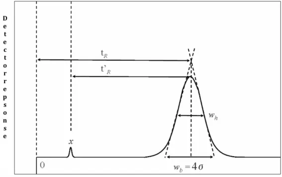
Resolution on magnetic sector instruments is normally given according to the 10% valley definition, which defines Δm by the mass difference between two resolved peaks with a 10% valley between them. The 10% valley definition is equivalent to that where Δm is defined by the peak width at 5% peak height (figure 1.5).

The most commonly used method to measure the resolution of quadrupoles, FT-ICR, orbitrap and TOF follows the full width at half maximum (FWHM) definition, which uses the width of a peak at 50% of its height as a measure for Δm (figure 1.5).

Figure 1.5. Examples of different definitions of resolution.

Instruments capable of low resolution (LR) operates at a R= 500– 2000. High resolution (HR) refers to a R> 5000. However, there is no exact definition of these terms. Furthermore, one should be aware that increased settings of resolving power are usually obtained at the cost of transmission of the analyzer, thereby reducing the absolute signal intensity.

Mass Spectrometry: Fundamental and Instrumentation

14

1.3.2 Mass accuracy

In mass spectrometry, resolution and accurate mass measurements are closely related to each other, because mass accuracy tends to improve as peak resolution is improved. However, a high-resolution measurement does not necessarily implies measuring the accurate mass, as the former aims to separate adjacent signals, while accurate mass measurements can deliver molecular formula determination [24,25]. The newly developed orbitrap and the new generation of orthogonal acceleration time-of-flight analyzers contributed to an increased demand for accurate mass data.

There are different ways to define and thus to calculate the mass of an atom, molecule or ion. Basically, an element is specified by the number of protons in its nucleus, i.e., the atomic number, which determines its place within the periodic table of the elements. Atoms with nuclei of the same atomic number but differing in the number of neutrons, i.e., by the mass number, are termed isotopes [23]. Those elements, which do exist in the form of only one single naturally occurring stable isotope, are termed monoisotopic elements. The distribution of the isotopic composition in a mass spectrum is named the isotopic pattern.

For stoichiometric calculations, chemists use the average mass that is the result of the weighted average of the atomic masses of the different isotopes of each element in the molecule. In mass spectrometry, the nominal mass is generally used; the latter being calculated using the mass of the predominant isotope of each element rounded to the nearest integer value. However, the exact masses of isotopes are not exact whole numbers. They differ weakly from the nominal mass by a determined value, so-called mass defect, which is unique for each isotope. The monoisotopic mass is then calculated by using

Mass Spectrometry: Fundamental and Instrumentation

15

the exact mass of the most abundant isotope for each constituent element. It is very close to but not equal to the nominal mass of the isotope. As a consequence, almost no combination of elements in a molecular formula has the same calculated exact mass as any other one. The only exception is the carbon isotope 12_{C, whose mass has been assigned precisely 12 u.}

As an example, the molecular ions of nitrogen, N2+•, carbon monoxide, CO+•,

and ethene, C2H4+•, have the same nominal mass of 28 u, i.e., they are

so-called isobaric ions. The isotopic masses of the most abundant isotopes of hydrogen, carbon, nitrogen, and oxygen are 1.007825 u, 12.000000 u, 14.003074 u, and 15.994915 u, respectively. Thus, the calculated exact masses are 28.00559 u for N2+•, 27.99437 u for CO+•, and 28.03075 u for C2H4+•. This

means they differ by several 10–3 u, and none of these isobaric ions measure precisely 28.00000 u.

The type of mass measured by mass spectrometry depends largely on the resolution and accuracy of the analyzer.

1.3.2.1 Exact mass and role of the electron mass

The exact mass of a positive ion formed by the removal of one or more electrons from a molecule is equal to its monoisotopic mass minus the mass of the electron, m_e[23]. The question is whether the mass of the electron me (5.48×10–4 _{u) has really to be taken into account. It strictly depends on the}

level of mass accuracy which is required. In fact, in FT-ICR, orbitrap, and orthogonal acceleration ToF (oaToF) instruments, which deliver mass accuracies in the order of <10-3u, one should definitely include the electron mass in exact mass calculations [26], as otherwise it could generate a

Mass Spectrometry: Fundamental and Instrumentation

16

considerable mass error.

1.3.2.2 Mass accuracy and determination of molecular formulas

The mass accuracy indicates the deviation of the instrument’s response between the measured accurate mass and calculated exact mass. It can be expressed as absolute mass accuracy, Δm/z:

𝛥𝑚/𝑧 = 𝑚 𝑧()*–

𝑚

𝑧,-.

or, alternatively, as relative mass accuracy, δ m/m, i.e., the absolute mass accuracy divided by the exact mass, and expressed as parts per million (ppm):

𝛿 𝑚 𝑚 = (𝛿𝑚/𝑧)/(𝑚/𝑧) ∗ 105

Accurate mass measurements allow to determine the elemental composition of an analyte, and thereby to confirm the identification of target compounds or to support the identification of unknowns. Assuming infinite mass accuracy, we should be able to assign the molecular formula of any ion simply through its exact mass. In reality, deviations between the accurate and exact mass of an ion always exist to some extent and, thus, we normally deal with errors in the order of one to several ppm depending on the type of instrument and the mode of its operation. Whatever the type of instruments or operation mode may be used, the assignment of molecular formulas must follow two general rules: i) it must always be in accordance with the experimentally observed; ii) the formula has to obey the nitrogen rule.

Mass Spectrometry: Fundamental and Instrumentation

17

1.3.2.3 High-mass molecules – influence of resolution on isotopic pattern and mass accuracy

Terms such as large molecules, or high mass, generally refer to masses in the range of 103_–104 _{u or above. By increasing m/z, the centre of the isotopic}

pattern is shifted to values higher than the monoisotopic mass. The center, i.e., the average mass, tends to be close to the peak of the most abundant mass. The monoisotopic mass is of course still related to a real signal, but it may be of such a low intensity that it is difficult to recognize [27]. It is certainly desirable to have at least sufficient resolution to resolve isotopic patterns of high-mass molecules, in order to be able to measure its monoisotopic mass. However, not every mass analyzer is capable of doing so. Mass analyzers such as quadrupole, time-of-flight or quadrupole-ion trap often generate some changes in spectral appearance thus affecting the actual measured mass [28]. For example, figure 1.6 illustrates the isotopic pattern of bovine insulin [C254H378N65O75S6]+ calculated at R= 1000, 4000, and 10,000. At R = 1000,

the isotopic peaks are not resolved and smoothly covered by an envelope. At

R = 4000, the isotopic peaks become almost sufficiently resolved. Finally, at R = 10,000, the isotopic pattern is well resolved and interferences between

isotopic peaks are avoided.

With regard to mass accuracy and determination of molecular formulas, it has been demonstrated that unequivocal formula assignment only works in a range up to about m/z 500 [29]

Mass Spectrometry: Fundamental and Instrumentation

18

Figure 1.6. Bovine insulin: isotopic pattern calculated for [M+H]+ at different resolutions.

In fact, a high level of mass accuracy measurement is unattainable if the peak shape is abnormal, due to instrumental reasons or unresolved isotopic envelopes, that is the case of large molecules. It has been reported that accuracy is limited to ± 0.1 Da for masses below 10 kDa [30], and with instruments capable of achieving ±0.5−5 ppm mass accuracy, that is necessary to distinguish peptide elemental compositions, it is possible to match homologous proteins having > 70% sequence identity [31]. Others have reported that, even at a high mass accuracy of 1 ppm, and with the particular case of peptides, the elemental composition can only be unambiguously identified up to about 800 u [32].

1.4 Instrumentation

“A modern mass spectrometer is constructed from elements which approach the state-of-the-art in solid-state electronics, vacuum systems, magnet design,

Mass Spectrometry: Fundamental and Instrumentation

19

precision machining, and computerized data acquisition and processing” [33]. This is and has ever been a fully valid statement about mass spectrometers. The basic type of mass spectrometer consists of three major parts: the ion source, the mass analyzer, and the detector. All mass spectrometers require low pressures (vacuum) conditions for operation. This is necessary to allow ions to survive along their path inside the mass spectrometer, and to reach the detector without undergoing collisions with other gaseous molecules. Indeed, collisions would produce a deviation of the ion trajectory and, in the worst case, its loss through the hitting of the mass analyzer surfaces. Besides, ion– molecule collisions could produce unwanted secondary reactions and hence increases the complexity of the spectrum. Introducing a sample into a mass spectrometer requires its transfer from atmospheric pressure into a region of high vacuum. An efficient pumping system uses mechanical pumps, which allow a vacuum of about 10−3 Torr to be obtained, in conjunction with turbo molecular pumps that allows a vacuum as high as 10−10 Torr to be reached. Furthermore, mass spectrometry can be coupled with separation methods such as gas chromatography (GC) and liquid chromatography (LC). “Hyphenation”, i.e., as GC-MS or LC-MS, delivers high selectivity and low detection limits for the analysis of trace compounds, or the possibility to resolve complex samples. In such a case, the mass spectrometer would act as the chromatographic detector, and its output must somehow represent the chromatogram that would have been obtained with other chromatographic detectors, e.g., flame ionization (FID), thermal conductivity (TCD) and ultraviolet detectors (UV).

Summarizing, a mass spectrometer should always perform the following processes: 1) produce ions from the sample in the ionization source; 2)

Mass Spectrometry: Fundamental and Instrumentation

20

separate these ions according to their mass-to-charge ratio in the mass analyser; 3) eventually, fragment the selected ions and analyze the fragments in a second analyser; 4) detect the ions emerging from the last analyzer, measure their abundance, and convert the ions into electrical signals; 5) process the signals coming from the detector through a computer.

1.4.1 Ion sources

In the ion source, the sample is ionized in the gas phase prior to analysis in the mass spectrometer. The choice of the ion source depends on the application, the internal energy transferred during the ionization process and the physic-chemical properties of the analyte that can be ionized. Some ionization techniques, so-called “hard”, are very energetic and cause extensive fragmentation of the analyte with even loss of its intact ion. Electron ionization belongs to such a group of sources. On the contrary, so-called “soft” ion sources, e.g., chemical ionization, do allow for generating intact ions of the molecular species. However, it is worthy to say that both EI and CI sources are only suitable for gas phase ionization, and thus their use is limited to sufficiently volatile and thermally stable compounds. In fact, when dealing with large non-volatile fragile (bio) molecules, that is the case of proteins, nucleic acids, polymers, it is necessary to introduce them into the vacuum of the mass analyzer after a process of nebulization of the containing solution (i.e., in ESI, APCI and APPI) or, alternatively, to bring them from the solid-state to the gas phase directly into the ion source housing, usually by means of a matrix (either solid or liquid) which promote both desorption and ionizations of the intact analytes. That is the case of MALDI and FAB. The number of available ion sources is quite large, even some of them are no longer commonly used today, but are of historical interest. Among them,

Mass Spectrometry: Fundamental and Instrumentation

21

electron ionization deserves an extensive treatment, given that its invention dates back to the infancy of mass spectrometry in the early 20th century [34].

1.4.1.1 Electron ionization (EI) ion sources

EI was introduced in 1921 by Dempster, who used it to measure lithium and magnesium isotopes [35]. Figure 1.7 illustrates a schematic representation of the electron ionization source. It consists of a chamber, so-called ionization chamber, which is region of the ion source block where analyte molecules are directly introduced and ionized. A resistively heated metal filament, typically made of rhenium or tungsten, creates the electron beam. The high-energy electrons produced are accelerated towards an anode and collide with the gaseous molecules to affect their ionization.

Mass Spectrometry: Fundamental and Instrumentation

22

Each electron has a given wavelength. If one of the frequencies has an energy corresponding to a transition in the molecule, an energy transfer that leads to various electronic excitations can occur. When there is enough energy, an electron can be expelled. The electrons do not “impact” molecules. For this reason, the former term electron impact has been correctly re-named as electron ionization. At the end of such an interaction, typically positive radical molecular ions are formed. For positive ions the electron energy is in most cases set to 70 eV. However, between only 10 and 20 eV energy is transferred to the molecules during the ionization process. The obvious consequence is that the excess energy leads to extensive fragmentation, which can be advantageous as it provides structural information for the elucidation of unknown analytes. Moreover, since the EI-mass spectra are relatively reproducible, a compound fingerprint scan be recorded, and that has triggered the construction of mass spectral databases for a quick and reliable compound identification.

Fragmentation can be more or less limited by lowering the electron energy. For example, using 12–15 eV electrons, instead of 70 eV, extended fragmentations are reduced. On the other hand, unfortunately, there is the considerable drawback of a general loss of intensity due to the decrease in ionization efficiency.

Nevertheless, during the first years of mass spectrometry, low- energy EI spectra were the only way to achieve mass spectra with a minimized fragmentation. It was only in the 1960s that chemical ionization was introduced as a valid technique in mass spectrometry for its “softness” features [36]

Mass Spectrometry: Fundamental and Instrumentation

23

energy. Thus this technique presents the advantage of yielding a spectrum with less fragmentation in which the molecular species is preserved. Consequently, C.I. can be considered as complementary to electron ionization. The ionization process is based on a chemical reaction between the analyte and an “ion reagent”, formed by subjecting to EI reagent gas molecules introduced in the source in large excess. This excess, which determines pressure in the source higher than those used in the EI, ensures that an electron entering the source block will preferentially ionize the reagent gas molecules, and that the resulting ions will mostly collide with other gas molecules. Subsequent ion-molecule interactions, by means of complex reactions involving proton transfer, hydride abstractions, adduct formations, charge transfers, and so on, will produce positive and negative ions of the substance, the latter particularly useful to analyze highly electronegative compounds.

1.4.1.2 Sample introduction

A sample introduction system has the function of transferring the analyte from their physical state and atmospheric conditions into low-pressure ion source. The type of sample inlet depends, strictly, on the type of sample to be analysed.

The reference inlet system instead, introduces the mass calibrant to perform the calibration of the system for accurate mass measurements.

A chromatography system can be coupled to a mass spectrometer, thus operating as a sample introduction system. This coupling also provides a second dimension to the chromatographic analysis, in terms of information. Coupling on-line a chromatograph with a mass spectrometer implies that the mobile phase, liquid or gas, has to be selectively removed while preserving the analyte as much as possible [37]. The first coupling between gas

Mass Spectrometry: Fundamental and Instrumentation

24

chromatography and mass spectrometry was realized at the end of the 50s [38]. Over the last decades, many efforts have been performed towards the development of proper interfaces capable to perform such a demanding task and to ensure the best throughput. Among them, electrospray ionization, atmospheric pressure chemical ionization and photoionization, each of them following different operations, marked the breakthrough in the feasible coupling between LC and MS.

1.4.1.3 Databases of EI mass spectra

In order to analyze a complex mixture, a separation technique is coupled with the mass spectrometer, provided that the separated compounds must be introduced one after the other into the spectrometer. The most obvious advantage consists of obtaining a spectrum that can be used to identify the separated compounds.

Within the context of GC-MS, low- and medium-polarity analytes are usually well suited for EI, while highly polar or even ionic compounds, e.g., diols or polyalcohol, amino acids, organic salts, should be properly derivatized [39,40]. In any case, EI mass spectra are excellently reproducible when measured under standard conditions (70 eV, ion source at 150–250°C), in both cases of measurements performed on the same or different types or brand of instruments. This fact has triggered the construction of mass spectral databases, commonly named as libraries. The most comprehensive EI mass spectral databases are those provided by the National Institute of Standards and Technology (NIST), and the Wiley/NBS [41]. Furthermore, the 2017 version of the NIST/EPA/NIH mass spectral database is equipped with a compilation of Linear Retention Index (LRI) values determined on non-polar and polar columns.

Mass Spectrometry: Fundamental and Instrumentation

25

1.4.2 Mass analyzers

A mass analyzer is a device that enables to separate the gas phase species produced according to their mass.

There are several types of mass analyzers used in mass spectrometric research that use different physical principles. They can be divided into two broad classes on the basis of many properties. Scanning analyzers allow only the ions of a given mass-to-charge ratio to go through at a given time. They are either magnetic sector or quadrupole instruments. On the contrary, mass analyzers such as time-of-flight, ion trap, ion cyclotron resonance or orbitrap, allow the simultaneous transmission of all ions across a given mass range. Analyzers can be also grouped on the basis of other properties, for example ion beam vs. ion trapping types, or continuous beam vs. pulse based.

Another trend in mass analyzer development is to combine different analyzers in sequence in order to allow multiple experiments to be performed. For example, triple-quadrupoles and more recently hybrid instruments such as quadrupole-TOF allow the generation of fragments over several decomposition experiments (MSn).

The main characteristics for measuring the performance of a mass analyzer are: 1) the mass range limit; 2) the analysis speed; 3) the transmission; 4) the mass accuracy and finally 5) the resolution.

Table 1.1 contains an overview of the analyzers available in mass spectrometry. In the context of the present thesis, two types of mass analyzers have been used, namely single quadrupole (qMS) and ion mobility Q-ToF (IM-Q-ToF)

Mass Spectrometry: Fundamental and Instrumentation

26

1.4.2.1 Quadrupole mass spectrometers

Quadrupole instruments are probably the most widely used type of mass spectrometer (Figure 1.8). The principle of the quadrupole mass analyzer was first by described by Paul and Steinwegen in 1953 [18]. A quadrupole consists of four precisely matched parallel metal rods. The mass separation is accomplished by the stable vibratory motion of ions in a high-frequency oscillating electric field that is created by applying direct-current (DC) and radio frequency (RF) potentials to these electrodes [42,43,44]. Opposite rods are connected electrically in pairs. The two pairs will, at any given time, have potentials of the same magnitude, but of opposite sign. Ions entering the space between the rods oscillate in the directions x and y, whose amplitude depends on the frequency of the potential applied and the masses of the ions. A positive ion will be attracted towards a negative rod. If the potential changes sign, the ion will change direction avoiding to discharge itself on the rod.

At given values of the DC and RF potentials, only ions within a certain narrow

m/z range will have stable trajectories and be allowed to reach the detector.

The motion of an ion traveling through the quadrupole is described by an equation established in 1866 by the physicist Mathieu, so-called Mathieu equation [45]. The DC potential applied to the electrodes of the X-Z plane is positive, while that applied to the electrodes of the Y-Z plane is negative. To understand the influence of potential on the trajectory at which a charged particle undergoes, it is convenient to examine the X-Z and Y-Z planes separately.

Mass Spectrometry: Fundamental and Instrumentation

27

Table 1.1. Common mass analyzers available in mass spectrometry.

Let’s start from X-Z plane (Figure 1.9). At positive (DC) potentials, ions will be rejected and focused toward the central axis of the electrodes.

When the potential is switched to negative value, the beam of positive ions will be accelerated towards the electrodes. If the potential at the electrodes changes rapidly, heavy ions will preferably be affected by the positive DC component, which means that they will be forced to move towards the middle between the electrodes. Conversely, in the presence of lighter ions, the negative, tough brief, potential can be sufficiently intense to attract and lead them to collide with the electrode. In such a X-Z plane configuration, one pair of rods will act as a “high pass mass filter”. In the Y-Z plane, the situation is similar except from the fact that the DC potential is negative.

Mass Spectrometry: Fundamental and Instrumentation

28

Figure 1.8. Schematic of the quadrupole analyzer.

The obvious consequence is that high-mass ions will preferably experience an attractive force and will hit one of the electrodes. On the contrary, tough low-mass ions also experience an attractive force most of the time, they are light enough to respond to the positive potential, and thus will be pushed back towards the middle between the electrodes. In this way, the rods act as a “low pass mass filter”.

Figure 1.9. Schematic representation of the motion of the ions inside the quadrupole

analyzer.

Mass Spectrometry: Fundamental and Instrumentation

29

the kinetic energy of the ions leaving the source. The only requirements are: i) the time for ions to go through the analyzer is short compared with the time necessary to switch from one mass to the other, and ii) the interscan delay, i.e., the time between one scan and the next, has to be small. Quadrupole analyzers generally are operated at unit resolution, thus restricting their use to low resolution applications. The mass range depends on the settings of the DC and RF voltages. Typical m/z ranges are 25 to 2000 u with unit mass resolution. Commonly to scanning analyzers, the quadrupole detects one ion at any given time, so most of the ions produced are not detected, thus decreasing the sensitivity. The sensitivity can be vastly improved when scanning a narrow m/z range, or operating in single ion monitoring (SIM) mode, namely choosing only on or few ions to be detected. In such an operation mode, the quadrupole mass spectrometer has a duty cycle of 100%.

The quadrupole mass analyzer has a relatively good dynamic range, which means that the quantification capabilities are generally very good. Thus, quadrupoles are preferably chosen alternatively to magnetic sectors which, tough more stable, are definitely costlier.

Because of the scanning property of quadrupole mass analyzers, they are well suited for continuous ion sources such as EI and ESI, but are not suitable for pulsed ionization methods. They are very often used in combination with GC and LC, and single (q) or triple quadrupole (QqQ) mass spectrometers are nowadays very common benchtop instruments for routine measurements.

1.4.2.2 Time-of-flight spectrometers

The concept of time-of-flight (TOF) analysers was described by Stephens in 1946 [46]. Wiley and McLaren published in 1955 the design of a linear TOF

Mass Spectrometry: Fundamental and Instrumentation

30

mass spectrometer which later became the first commercial instrument [47]. The principle of TOF is quite simple: ions of different m/z are dispersed in time during their flight along a field-free drift path of known length. All ions start at the same time or at least within a sufficiently short time interval and the lighter ones will arrive earlier at the detector than the heavier ones.

The first-generation TOF instruments were designed for coupling with gas chromatography; however, linear quadrupole analyzers soon surpassed it. Only in the end of 1980s there was a renewed interest in TOF analyzer thanks to the new-pulsed ionization methods and the development of matrix-assisted laser desorption/ionization sources (MALDI) [48]. TOF analyzers were adapted for use with other ionization methods and are now even strong competitors to the well-established magnetic sector instruments in many applications. [49,50,51].

Figure 1.10 shows the scheme of a linear TOF instrument. Ions are expelled from the source in “packages” by a transient application of the required potentials on the source focusing lenses. These ions are then accelerated towards the flight tube by a difference of potential applied between an electrode and the extraction grid. When this ions leaving the acceleration region, they will have the same charge and, ideally, the same kinetic energy, and will enter into a field-free region where will be separated according to their velocities, and reach the detector positioned at the other extremity of the flight tube. Provided that all the ions start their journey at the same time, or at least within a suitable short time interval, the lighter ones will arrive earlier at the detector than the heavier ones.

Mass Spectrometry: Fundamental and Instrumentation

31

Figure 1.10. Schematic representation of a linear TOF mass spectrometer.

Such an instrumental setup where the ions are traveling on a straight line from the point of their generation towards the detector is called “linear” TOF. The time difference between the starting signal of the pulse and the time at which an ion hits the detector is the time of flight (TOF) and can be expressed as:

𝑡₇₈₉ = 𝐿 𝑣 = 𝐿

𝑚

2𝑞𝑈_- ∝ 𝑚 𝑧

where L is the length of the field-free region, v is the ion velocity after acceleration, m is the mass of the ion, q the charge of the ion, Ua the

accelerating electric potential difference, and z the charge state. This equation shows that, higher is the mass of an ion slower it will reach the detector, and vice versa.

In principle, the upper mass range of a TOF analyzer has no limit, which makes it especially suitable for analyzing large molecules, e.g., up to 300 kDa [52].

Another advantage of these instruments is their high transmission efficiency which leads to very high sensitivity compared to quadrupole and sector analyzers. That is because all the mass range is simultaneously analyzed

Mass Spectrometry: Fundamental and Instrumentation

32

contrary to the scanning analyzers where ions are transmitted successively along a time scale.

Generally, the TOF analyzer is very fast, and a spectrum over a broad mass range can be obtained in the microseconds time interval. As the mass resolution is proportional to the flight time and the flight path, one solution to increase the resolution of these analysers is to lengthen the flight tube. However, too long a flight tube decreases the performance of TOF analysers because of the loss of ions by scattering after collisions with gas molecules or by angular dispersion of the ion beam. It is also possible to increase the flight time by lowering the acceleration voltage. But lowering this voltage reduces the sensitivity. Therefore, the only way to have both high resolution and high sensitivity is to use a long flight tube with a length of 1 to 2 m for a higher resolution and an acceleration voltage of at least 20 kV to keep the sensitivity high.

The most important drawback of the first TOF analysers was their poor mass resolution. Mass resolution is affected by factors that create a distribution in flight times among ions with the same m/z ratio. These factors are: i) different time distribution; ii) different in space distribution and iii) different kinetic energy distribution. These drawbacks are substantially improved with the development of two techniques: delayed pulsed extraction and the reflectron.

1.4.2.2.1 Reflectron

As aforementioned a way to improve mass resolution is to use an electrostatic reflector also called a reflectron. The reflectron was proposed for the first time by Mamyrin [53]. It creates a retarding field that acts as an ion mirror by deflecting the ions and sending them back through the flight tube. The term reflectron time-of-flight (RTOF) analyser is used to differentiate it from the

Mass Spectrometry: Fundamental and Instrumentation

33

linear time-of-flight (LTOF) analyser. The simplest type of reflectron, which is called a single-stage reflectron, consists usually of a series equally spaced grid electrodes or more preferably ring electrodes connected through a resistive network of equal-value resistors.

As shown in Figure 1.11 the reflectron is situated behind the field-free region opposed to the ion source while detector is positioned on the source side of the ion mirror to capture the arrival of ions after they are reflected. The reflectron corrects the kinetic energy dispersion of the ions leaving the source with the same m/z ratio. Consequently, ions with more kinetic energy and hence with more velocity will penetrate the reflectron more deeply than ions with lower kinetic energy. Consequently, the faster ions will spend more time in the reflectron and will reach the detector at the same time than slower ions with the same m/z. Although the reflectron increases the flight path, though without increasing the dimensions of the mass spectrometer, the beneficial increase in mass resolution comes at the expense of sensitivity and mass range limitation. The choice of operating TOF instruments in “linear” or “reflectron” mode heavily depends on the species to be detected. For example, when operating in linear mode, the aim is usually to detect larger species, which will not be stable enough to survive along the strong electric field of the reflectron. Therefore, the given resolving power is much lower, as the width of the isotopic envelope do not allow for its decent resolution. The opposite is the case of ReTOF, because especially in the presence of metastable fragmentations (i.e., in tandem MS), only fragments still having kinetic energies close to that of the precursor can be successfully and sensitively detected.

Mass Spectrometry: Fundamental and Instrumentation

34

1.4.2.2.2 Orthogonal acceleration.

The major breakthrough in the technological development of TOF analyzers arose from the design of the orthogonal acceleration TOF analyzer (oaTOF). In an oaTOF analyzers, pulses of ions are extracted orthogonally from a continuous ion beam. Specifically, ions fill the first stage of the ion accelerator in the space between the extraction plate and a grid. A pulsed electric field is then applied at a frequency of several kilohertz, which force ions to assume a direction orthogonal to their original trajectory, and then begin to fly towards the analyzer. The most significant advantages of oaTOF analyzers are: i) high mass resolving power, and ii) mass accuracies even up to or below 1 ppm. Therefore, it is not surprising that oaTOF instruments are currently widespread used in combination with GC and fast GC.

Figure 1.11. The working principle of a single-stage reflectron.

1.4.2.3 Ion mobility spectrometers

Mass Spectrometry: Fundamental and Instrumentation

35

technique for the separation and subsequent detection of volatile and semi- volatile organic compounds based on the separation of their gaseous ions in a low or high electric field at ambient pressure. The first coupling of ion mobility to MS is attributed to McDaniel who, between the 1950s and 1960s, developed drift cells coupled to a magnetic sector mass analyzer, with the objective of studying ion mobility and ion-molecule reactions [54] IMS enables the discrimination of ions by size, shape, charge as well as mass, thus providing additional information to the chromatographic separation of molecules and mass spectrometric separation of ions. Four methods of ion mobility separation can be combined with MS, namely drift-time ion mobility spectrometry (DTIMS), aspiration ion mobility spectrometry (AIMS), differential-mobility spectrometry (DMS) also called field-asymmetric waveform ion mobility spectrometry (FAIMS) and traveling- wave ion mobility spectrometry (TWIMS).

Ions exposed to an electric field experience a force and are accelerated along the field lines. Upon addition of a buffer gas, the motion of the ions becomes more complicated as collisions with the gas scatter the ions in random directions as it diffuses. However, if an ion cloud is given enough time to reach equilibrium and the electric field is uniform throughout, the ion cloud will travel with constant velocity parallel to the field lines and simultaneously grow in size due to diffusion. This constant equilibrium velocity is the result of forward acceleration by the field and decelerating friction by collisions. Following Mason and McDaniel [55], for weak electric fields of magnitude E, the drift velocity v is directly proportional to E with the proportionality constant K called ion mobility

Mass Spectrometry: Fundamental and Instrumentation

36

Since v is inversely proportional to the buffer gas number density N, the mobility K is also inversely proportional to N. Here N (in units of molecules per volume) is used as the relevant quantity to express pressure because N is, in contrast to pressure p, decoupled from the temperature T. Because K depends on N it is practical to convert K into the pressure-independent quantity

Ko

∝

𝐾_D = 𝑝 𝑝_D =

𝑇_D

𝑇 𝐾 (𝟏. 𝟐) with the constants p_o = 760 Torr and T_o = 273.15 K.


A field is considered weak if the average ion energy acquired from the field is small compared to the thermal energy of the buffer gas molecules. This ion field energy is proportional to v2 or (KE)2. However, for a given ion with given

Ko ∝NK it is the ratio E/N which determines whether a field is weak or strong, and collisional heating due to the field is given by equation

𝑇_HII− 𝑇 = (𝑀/3𝑘_N) 𝑁𝐾 P_(𝐸/𝑁)P _{(𝟏. 𝟑)}

Here T_eff is the effective temperature, M the mass of the buffer gas particle, and kB the Boltzmann constant.

Following Equation (1.1), a measurement of K involves measuring the drift time t of a pulse of ions traveling in a weak field E over a given drift length L. The spread, Δx, of a cloud of identical ions due to diffusion, the random part of motion, is given by

Mass Spectrometry: Fundamental and Instrumentation

where e is the ion charge and V the voltage across the drift region.

Because the resulting acceleration of the ion by E is proportional to e, the mobility is also proportional to e. In addition, because the deceleration of the ion by friction is proportional to the buffer gas number density N and because large ions experience more friction than small ions, the mobility is inversely proportional to both N and the collision cross section σ of the ion. Using momentum transfer theory, a statistical approach to balance ion energy and momentum gained in the electric field and lost in buffer gas collisions, a quantitative relationship between K and the quantities e, N, and σ can be derived, 𝐾 = 3𝑒 16𝑁 2𝜋 𝑘_N𝑇 1 𝜎 (𝟏. 𝟓)

where µ = Mm / (M + m) is the reduced mass of buffer gas (with mass M) and ion (with mass m).

1.4.2.3.1 Collision cross section

Ion mobility separations are based on differences in ion structures (or cross sections) and charge states. The latter is established by the excess charge on each species. Ion cross sections represents the effective area for the interaction between an individual ion and the neutral gas through which it is travelling [56]. Two ions of equal mass and charge, but different three-dimensional conformation, will travel through an IMS device at velocity dependent on their mobilities, providing different drift times. Specifically, the ion with a more

Mass Spectrometry: Fundamental and Instrumentation

38

compact conformation will undergo fewer collisions with the neutral gas than do more open. Therefore, compact species with small collision cross sections (CCS, Ω) will have higher mobilities than do more open forms of the ion. The mobility can be used to obtain a CCS for a specific ion according to the Mason-Schamp equation [57] where K0 is the reduced mobility (measured

mobility at standard temperature and pressure), z is the charge state of the ion,

e is the elementary charge, N is the number density of the drift gas,

Ω = 3𝑧𝑒 16𝑁 2𝜋 𝜇𝑘_N𝑇 ] P 1 𝐾_D (𝟏. 𝟔)

µ is the reduced mass of the ion-neutral drift gas pair, k_B is the Boltzmann constant and T is the gas temperature. The proportional relationship between

Ω and K0 is true for value equal or under the “low-field limit”, where the ratio

between electric field strength and buffer gas density is small than 2×10–17 V cm2 [58]. Despite the IMS devices previous discussed will all separate ions according to differences in their mobility through a buffer gas, only the time-based mobility devices (DT-IMS, TW-IMS) can be used to determine information about cross- sectional area.

1.4.2.3.2 Resolution

The resolution of an IMS device depends in practice not only on the spread of ions Δt due to diffusion in the drift region relative to the drift time t, but also on the drift tube-independent spread of the ion cloud, Δto, brought about by

the initial width of the ion pulse entering the drift region and the spread of ions after the drift region (e.g., in the ion funnel). Following Equation (1.4), the resolution t/Δt is affected only by the two parameters: temperature T and drift voltage V.

Mass Spectrometry: Fundamental and Instrumentation

Reducing T decreases diffusion and thus Δt. Increasing the voltage reduces both t and Δt, with the ratio t/Δt being proportional to 𝑉 𝑇. However, whereas increasing L is a reasonable approach to improve resolution, increasing E requires simultaneous increase in N in order to keep E/N constant and to stay in the low-field regime desirable for ion mobility experiments. For high-resolution devices the pulse width Δto may be an additional limitation to

resolution. Once Δt reaches a small value and the resolution is determined by Δto, further optimization of the parameters E, N, and T does not further

improve the resolution. Hence the design of an ion mobility instrument requires a careful balance of ion energy, technical feasibility, and all the quantities determining the resolution. High voltage supplies, insulators, and discharge problems set limits to V; discharge and pumping requirements may set limits to N; space requirements set limits to L; choice of materials, insulation, discharge due to water condensation, and thermal equilibration set limits to T; and speed of switches, ion space charge, and signal intensity set limits to Δt_o.

Therefore, an instrument with given fixed parameters L, Δto, and T and with

maximum allowable pressure N may operate with maximum resolution at a field value Emax smaller than the instrument limit and smaller than allowed due

to E/N limitations. Hence whereas the resolution is optimum for E = Emax, it

drops both for E <Emax due to smaller t/Δ t ∝

a

7 values [Equation (1.7)] and for E >Emax due to smaller t/Δ to∝t ∝ 1/E values [Equation (1.1)].

Mass Spectrometry: Fundamental and Instrumentation

1.4.3 Tandem mass spectrometry

The goals of any mass spectrometry analysis are to obtain more structural information on the analyte of interest, sometimes unattainable either (i) because the ionization technique used produces relatively few structurally diagnostic fragments (as for soft ionization), or (ii) because its fragmentation is suppressed by the presence of other compounds in the mixture introduced in the ion source, or (iii) because it is obscured by other ions generated from the matrix in the course of ionization. For such reason, the strong need of new techniques able to bypass these problems, and provide much valuable information about the molecular structure, led to development of tandem mass spectrometry. The term tandem mass spectrometry, or simply tandem MS, refers to any general methods where a given ion is subjected to a second mass spectrometric analysis, either in conjunction with a dissociation process or in a chemical reaction (59). Tandem MS is also defined as mass spectrometry/mass spectrometry (MS/MS). Several modern mass spectrometers consist of two or more mass analyzers to perform the so-called

tandem-in-space MS/MS, where different mass analyzers are involved “in

different spaces”. This MS/MS technology is based on the isolation of a specific precursor ion (m/z), and then undergone to dissociation and production of fragment or product ions. However, due to rapidly decreasing transmission and increased instrumental complexity and size, only MS/MS experiments are allowed, while MS3 experiments and beyond are rarely

Mass Spectrometry: Fundamental and Instrumentation

41

performed in tandem-in-space instruments. Systems such as QqQ, Q-ToF, ToF/ToF belong to such a tandem MS technique. In all these combinations, the first and the final analyzers operate the ion isolation and scan, whereas the second analyzer is a collision cell that allows ion fragmentation.

There are four mains MS/MS scan modes usually used: product ion scan, precursor ion scan, neutral loss scan, and selected reaction monitoring. In the product ion mode, the first analyzer selects a precursor ion of interest, which is fragmented into the collision cell, thus generating the product ions analyzed by the second analyzer. In the precursor ion scanning, the second analyzer is held static at the m/z of a specific product ion only after collision, whereas the first mass analyzer is scanned across the desired m/z range. This experiment results in a spectrum of precursor ions that produce that particular product ion during collision induced dissociation (CID) fragmentation. During the neutral loss scanning process, both the first and the second analyzer work in concert with a constant mass offset of “x”. When a precursor ion is transmitted through the first mass analyzer, this ion is recorded if it produces a product ion corresponding to the loss of a neutral fragment of ‘‘x’’ from the precursor ion after collision cell. In the selected reaction monitoring scan mode, the first analyzer is set on the specific precursor mass, the collision energy is optimized to produce a diagnostic fragment of that precursor ion, and the second analyzer focuses on the specific mass of that fragment. Only ions with this exact transition will be detected. This process is also known as multiple reaction monitoring (MRM) in the case of first or second or both mass analyzers are set to monitor for multiple reactions. This technique is broadly used for quantitative analysis of individual molecular species.

Along the tandem-in-space, the tandem-in-time is the other possible MS/MS method processing, which employs a single mass analyzer where ions are