Politecnico di Milano
School of Civil, Environmental and Land Management Engineering
BEF Element with Rigid Joints and Lumped Elasticity for
Structural Analysis of Axisymmetric Shells with Ring Beams.
Master Thesis by:
Juan Sebastian Garcia N.
Francesco Monachello A.
Supervisors:
Prof. Fabio Biondini
Dr. Andrea Titi
We thank Dr. Biondini and Dr. Titi for sharing their time and knowledge. Their guide was a reliable compass in moments of uncertainty. F. Monachello, J.S. Garcia
Dedicated to María Torcoroma, Fabiola, and Domingo for their love and example. Your support and patience during these years of preparation made this work possible. F. Monachello.
I dedicate this work to my father Duvan, my mother Manrry and sister Valentina for their constant support, understanding, sacrifices and love throughout these three years, to Andrea who always encouraged me to fight for myself and understand my abilities. J.S. Garcia
Abstract
The use of reliable computational tools is strictly required to proper analyse and design civil engineering structures. Such problem represents a key aspect in the study of shell structures, widely adopted in civil, hydraulic, mechanical and aeronautical engineering. In particular, in civil engineering they are used for liquid-retaining structures, storage silos, containment structures, cooling towers and arch domes, among others. These systems are characterized by some peculiarities, as for example the small thickness compared to the minimum radius of curvature of the midsurface. Moreover, the resisting mechanism to transverse loading is mainly based on the membrane resistance conferred by curvature, which makes this kind of structures very efficient. Analytical solutions for these systems are generally complex and limited to simple problems, especially due to boundary conditions. In particular, one of the most used solution has been proposed in the past by Geckeler (in the following indicated as Geckeler approximation), based on the observation that in shell structures horizontal forces or bending moments uniformly applied along the boundaries lead to displacements and internal actions for which amplitude exponentially decay far from the boundaries themselves. However, when the complexity of the problem increases, the use of computational models is the only practical way. To this purpose, present work is devoted to the implementation of a structural code for the analysis of generic shell structures, based on the analogy of the beam on elastic foundation (BEF). The novelties are represented by the development of shape functions to proper represent displacements and internal actions of a structure supported by elastic foundations and the modelling of the ring beam. A BEF element with rigid joints and lumped plasticity is formulated. The effectiveness of the proposed methodology is shown through the solutions of several applications, including reinforced concrete tanks subjected to pressure and hydrostatic forces.
Keywords: Axisymmetric shell structures, Geckeler approximation, ring beams, beam on elastic foundation (BEF) analogy, BEF shape functions, BEF with rigid joints and lumped elasticity.
Sommario
Una corretta analisi e progettazione di opere di ingegneria civile richiede l’utilizzo di strumenti di calcolo affidabili. Tale problematica assume un ruolo chiave nello studio di strutture a guscio, ampiamente utilizzate in applicazioni come serbatoi in pressione, serbatoi per lo stoccaggio di liquidi, silos e strutture a cupola. Tali strutture presentano peculiarità rilevanti quali il ridotto spessore rispetto al raggio di curvatura e una capacità di trasmissione del carico agente basata su un meccanismo prevalentemente membranale, tale da garantire un’elevata efficienza meccanica. Le soluzioni analitiche riportate in letteratura sono in genere complesse e limitate a geometrie semplici, soprattutto per quanto riguarda le condizioni al contorno. In particolare, ha trovato largo impiego un’espressione approssimata proposta da Geckeler (a cui ci si riferirà nel seguito come approssimazione di Geckeler) basata sull’osservazione che in gusci di rivoluzione sollecitati al bordo da forze radiali o momenti sforzi e deformazioni tendono a smorzarsi rapidamente allontanandosi dal bordo stesso. Tuttavia, all’aumentare della complessità del problema, l’utilizzo di modelli computazionali di comprovata affidabilità risulta l’unica soluzione percorribile. A tale scopo, il presente lavoro propone quindi l’implementazione di un codice di calcolo per l’analisi di strutture a guscio di geometria generica, basato sull’analogia della trave su suolo elastico. Le caratteristiche principali del lavoro di tesi riguardano lo sviluppo di opportune funzioni di forma in grado di rappresentare correttamente spostamenti e forze interne di una struttura che poggia su un letto di molle elastiche e la modellazione della trave ad anello. Viene in particolare formulato un elemento di trave su suolo elastico con nodi rigidi e elasticità concentrata. L’efficacia dell’approccio proposto viene mostrata mediante numerose applicazioni, tra cui serbatoi in pressione e per il contenimento dell’acqua.
Parole chiave: Strutture assialsimmetriche a guscio, Approssimazione di Geckeler, travi ad anello, trave su suolo elastico (BEF), funzioni di forma BEF, elemento BEF con nodi rigidi e elasticità concentrata.
Introduction ... 25
1 Basic Concepts for Axisymmetric Shells ... 37
1.1
Circular Cylindrical Shells ... 37
1.1.1
Kinematic Field ... 37
1.1.2
Static Field ... 37
1.1.3
Flexural Behaviour ... 38
1.1.4
Membrane Behaviour ... 39
1.1.5
Differential equation for flexural behaviour ... 40
1.2
Ring beams ... 45
1.3
Spherical Shells ... 50
1.3.1
Membrane Behaviour ... 50
1.3.2
Flexural Analysis ... 55
1.4
Conical Shells ... 59
1.4.1
Membrane Behaviour ... 60
1.4.2
Flexural Analysis ... 64
2 Beam on Elastic Foundation (BEF) Analogy ... 65
2.1
Theoretical Background ... 65
2.1.1
Winkler model stiffness matrix ... 67
2.1.2
Winkler model load vectors ... 70
2.2
BEF analogy for structural analysis of axisymmetric shells ... 71
2.2.1
Cylindrical tanks ... 72
2.2.2
Axisymmetric Spherical and Conical Shells ... 73
3 Implementation of BEF Analogy ... 77
3.1
Displacement field in Winkler Beam Model ... 77
3.1.1
Shape functions for Winkler Beam model ... 77
3.1.2
Shape functions implementation ... 82
3.1.3
Adequacy of shape functions to display displacements ... 84
3.1.4
Stresses in Winkler Beam Model ... 86
3.2
Cylindrical shell modelling ... 93
3.2.1
BEF element with ring beams ... 100
3.3
Spherical and Conical Shells modelling ... 104
3.3.1
Computational modelling topics for spherical shells ... 107
3.3.2
Modified load ... 112
3.3.3
Modified load method ... 118
3.3.5
Kinematic constraints ... 125
3.3.6
Validation of the modelling ... 128
4 Benchmarks ... 167
4.1
Benchmarks of Beam on Elastic Foundation ... 167
4.2
Benchmarks of Cylindrical shells ... 195
4.2.1
Cylindrical Tanks ... 195
4.2.2
Cylindrical Tank filled with water ... 204
4.2.3
Cylindrical Tank Constant Load ... 206
4.2.4
Cylindrical Tank Varying Thickness ... 209
4.2.5
Cylindrical Tank Partially Filled with Water ... 213
4.2.6
Cylindrical tank filled with water with stiffened base. ... 216
4.2.7
Cylindrical tank filled with water stiffened at top. ... 220
4.2.8
Cylindrical tank filled with water with different boundary conditions ... 225
4.2.9
Cylindrical tank filled with water stiffened at mid height. ... 235
4.2.10
Cylindrical tank filled with water with multiple ring beams. ... 244
4.3
Spherical Shells Benchmarks ... 249
4.3.1
Spherical Shell under constant pressure ... 249
4.3.2
Spherical shell under self-weight ... 252
4.3.3
Spherical shell under constant pressure with stiffened edge ... 256
4.3.4
Spherical shell under self-weight stiffened at the edge ... 261
4.3.5
Clamped spherical shell under constant pressure ... 266
4.3.6
Clamped spherical shell under constant pressure using modified load method 272
4.3.7
Clamped spherical shell under self-weight ... 275
4.3.8
Strip element modelling in spherical shells ... 280
4.4
Benchmarks for conical shells ... 283
5 Applications ... 287
5.1
Spherical shell under self-weight stiffened at its edge by a ring beam ... 287
5.2
Cylindrical pressure vessel with hemispherical roof ... 294
5.3
Cylindrical pressure vessel with spherical roof ... 301
5.4
Cylindrical storage tank with ring beam and spherical roof ... 310
6 Conclusions and future developments ... 327
7 Annex ... 329
7.1
Elastic Restraints ... 329
7.2
Multi point constraints ... 329
7.4
Symbolic Matrix for BEF element with ring beams ... 337
7.5
Segments of the Code ... 339
References ... 360
List of Figures
Figure 1.1. Cylindrical shell parameters. ... 37Figure 1.2. Forces on a differential of the shel ... 38
Figure 1.3. Internal stresses distribution in a strip. ... 38
Figure 1.4. Circumferential membrane forces distribution. ... 40
Figure 1.5. Forces on the strip of the cylindrical shell. ... 40
Figure 1.6. Wavelength at the edges. ... 42
Figure 1.7. Amplitude decay in a cylindrical shell. ... 43
Figure 1.8. Ring beam at bottom edge of cylindrical shell. ... 45
Figure 1.9. Actions transmitted between ring beam and cylinder. ... 45
Figure 1.10. Force method applied on ring beam with a) actual structure, b) the redundant forces on the tank and c) redundant forces on the ring beam. ... 46
Figure 1.11. Ring beam displacements from radial loads. ... 47
Figure 1.12. Ring beam displacements from applied bending moment. ... 48
Figure 1.13. Top and bottom fiber of the ring beam. ... 49
Figure 1.14. Spherical shell. ... 50
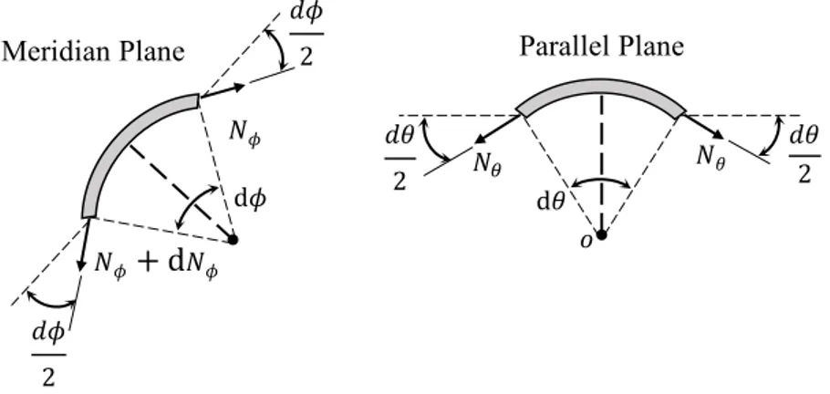
Figure 1.15. Differential element of spherical shell. ... 50
Figure 1.16. Displacements and external loads in a spherical shell segment. ... 51
Figure 1.17. Membrane forces in meridian and parallel planes. ... 51
Figure 1.18. Spherical shell under self-weight ... 52
Figure 1.19. Displacements on a segment of the spherical shell. ... 52
Figure 1.20. Spherical shell under gravitational loading. ... 53
Figure 1.21. Stresses corresponding to different types of loading. ... 54
Figure 1.23. Simply supported spherical shell edge flexural disturbances. ... 55
Figure 1.24. Horizontal edge forces. ... 56
Figure 1.25. Bending moment at edge. ... 56
Figure 1.26. Angular coordinates in a spherical shell. ... 58
Figure 1.27. Amplitude decay in a spherical shell. ... 58
Figure 1.28. Membrane stresses in conical shells ... 60
Figure 1.29. Differentials of a conical shell. ... 61
Figure 1.30. Membrane stresses for self-weight loading. ... 61
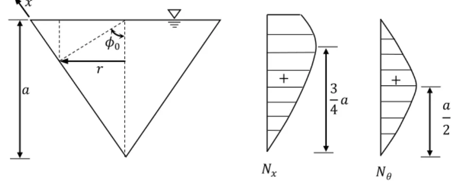
Figure 1.31. Membrane stresses hydrostatic pressure. ... 62
Figure 1.32. Membrane stresses for a truncated conical tank. ... 63
Figure 1.33. Truncated conical tank membrane force distribution. ... 63
Figure 1.34. Equivalent spherical shell in conical shell. ... 64
Figure 2.1. Foundations footings. ... 65
Figure 2.2. Design procedures for dynamically loaded foundations. ... 66
Figure 2.3. Beam on elastic foundation. ... 67
Figure 2.4. Beam on Elastic Foundation subgrade coefficients. ... 67
Figure 2.5. Beam element on elastic foundation under transversal and longitudinal loads ... 68
Figure 2.6. Flexural Behaviour ... 68
Figure 2.7. Axial Behaviour. ... 69
Figure 2.8. Equivalent nodal forces for Beam on elastic foundation. ... 70
Figure 2.9. Load effects on the beam element. ... 70
Figure 2.10. Beam on elastic foundation reaction of elastic bed. ... 71
Figure 2.11. Cylindrical tank discretization for BEF. ... 73
Figure 2.12. Conical Shell. ... 74
Figure 2.13. Spherical Shell analogy. ... 75
Figure 2.14. Discretization of a spherical shell strip. ... 75
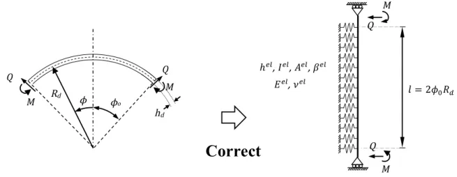
Figure 2.15. Correct discretization for a spherical shell strip. ... 75
Figure 3.2. Modelling of the shape function on Fortran. ... 83
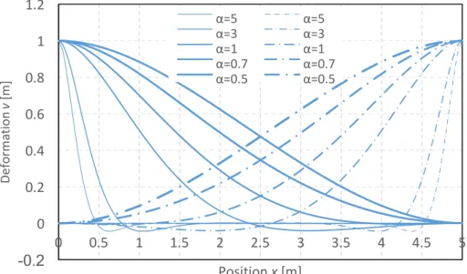
Figure 3.3. Displacement for different values of alpha. ... 84
Figure 3.4. Rigid body motion for different values of alpha. ... 84
Figure 3.5. Integral functions for shear. ... 91
Figure 3.6. Integral functions for bending moment. ... 92
Figure 3.7.Integra functions for axial component. ... 93
Figure 3.8. Representation of cylindrical shell by modelling on WBM ... 94
Figure 3.9. Different boundary conditions for cylindrical shells supports. ... 94
Figure 3.10. Variation of conditions along height. ... 95
Figure 3.11. Ring beam located at the top of the cylindrical shell. ... 95
Figure 3.12. Ring beam located at the bottom of the cylindrical shell. ... 96
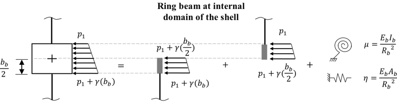
Figure 3.13. Ring beam located at other part of the domain. ... 96
Figure 3.14. Boundary conditions for a) roller at centroid or bottom fiber, b) simply supported at centroid, c) slider at centroid and bottom fiber and d) simply supported at bottom fiber. ... 99
Figure 3.15. BEF element with ring beam ends. ... 100
Figure 3.16. BEF element with ring beam ends a) End displacements and b) End forces ... 100
Figure 3.17. Arbitrary position of the centroid of the ring beam. ... 102
Figure 3.18. Unitary width strip. ... 104
Figure 3.19. Different approximation for the strip of the spherical shell. ... 105
Figure 3.20. Incorrect modelling of a spherical shell. ... 105
Figure 3.21. Correct modelling of spherical shell. ... 106
Figure 3.22. Conical shell modelling. ... 106
Figure 3.23. Subdivision of conical shell domain. ... 107
Figure 3.24 Relevant Kinematic coordinates ... 107
Figure 3.25. Boundary conditions at the edge. ... 108
Figure 3.26. Membrane forces for constant pressure load. ... 108
Figure 3.27. Membrane forces for snow load. ... 109
Figure 3.29. a) BEF element subjected to constant load b) Spherical shell subjected to constant
load. ... 113
Figure 3.30. Modified factor for constant pressure load case. ... 115
Figure 3.31. Modified factor for snow load case 𝜙𝑜 = 90. ... 116
Figure 3.32. Modified factor for constant pressure load case 𝜈 = 0.15. ... 116
Figure 3.33. Modified factor for self-weight case 𝜙𝑜 = 90. ... 118
Figure 3.34. Modified factor for self-weight case 𝜈 = 0.15. ... 118
Figure 3.35. Superposition principle for modified load method. ... 120
Figure 3.36. Reconstruction of bending behaviour. ... 120
Figure 3.37. Simply supported boundary condition. ... 121
Figure 3.38. Vertical reaction force computation. ... 121
Figure 3.39. Added radial component of vertical reaction. ... 122
Figure 3.40. Interaction between spherical and cylindrical shells in pressure vessels. ... 123
Figure 3.41. Radial effect due to vertical load. ... 124
Figure 3.42. WBM of a structure with cylindrical and spherical shell. ... 125
Figure 3.43. Radial displacement relation between spherical and cylindrical shell. ... 126
Figure 3.44. Interface modelling connecting two nodes. ... 126
Figure 3.45. Master and slave definition and proper boundary condition. ... 127
Figure 3.46. Clamped spherical shell under constant pressure. ... 128
Figure 3.47. Single finite element under constant pressure. ... 129
Figure 3.48. Displacement along the spherical shell. ... 130
Figure 3.49. Shear along the spherical shell. ... 130
Figure 3.50. Bending moment along the spherical shell. ... 130
Figure 3.51. Reconstruction of the flexural behaviour. ... 131
Figure 3.52. Displacement of the free BEF element. ... 131
Figure 3.53. Shear on the free BEF element. ... 132
Figure 3.54. Bending moment on the free BEF element. ... 132
Figure 3.56. Shear of the clamped spherical shell. ... 133
Figure 3.57. Bending moment of clamped spherical shell. ... 133
Figure 3.58. Hinged spherical shell. ... 134
Figure 3.59. BEF element for hinged spherical shell. ... 135
Figure 3.60. Displacement of hinged spherical shell. ... 135
Figure 3.61. Shear of hinged spherical shell. ... 136
Figure 3.62. Bending moment of hinged spherical shell. ... 136
Figure 3.63. Comparison of shear of hinged spherical shell. ... 137
Figure 3.64. Comparison of bending moment for hinged spherical shell. ... 137
Figure 3.65. Spherical shell with sliding supports under constant pressure. ... 138
Figure 3.66. BEF element for spherical shell with sliding supports under constant pressure. .. 138
Figure 3.67. Displacement for the free BEF element. ... 139
Figure 3.68. Shear of free BEF element. ... 139
Figure 3.69. Bending moment of free BEF element. ... 140
Figure 3.70. Simply supported spherical shell with 90 degrees opening. ... 140
Figure 3.71. Numerical model of simply supported spherical shell under constant pressure. .. 141
Figure 3.72. Displacement of simply supported spherical shell. ... 142
Figure 3.73. Shear of simply supported spherical shell. ... 142
Figure 3.74. Bending moment of simply supported spherical shell. ... 143
Figure 3.75. Clamped spherical shell under self-weight. ... 143
Figure 3.76. Numerical modelling of the clamped spherical shell under self-weight. ... 144
Figure 3.77. Displacement of the spherical shell under self-weight. ... 146
Figure 3.78. Shear of spherical shell under self-weight. ... 147
Figure 3.79. Bending moment of spherical shell under self-weight. ... 147
Figure 3.80. Free edge spherical shell model under self-weight. ... 148
Figure 3.81. Displacement of free edge spherical shell model under self-weight. ... 148
Figure 3.82. Shear of free edge spherical shell model under self-weight. ... 149
Figure 3.84. Corrected bending moment diagram of spherical shell under self-weight. ... 150
Figure 3.85. Corrected shear diagram of spherical shell under self-weight. ... 150
Figure 3.86. Shear diagram for 20 finite elements. ... 152
Figure 3.87. Bending moment diagram for 20 finite elements. ... 152
Figure 3.88. Shear diagram of clamped spherical shell under self-weight. ... 153
Figure 3.89. Bending moment diagram of clamped spherical shell under self-weight. ... 153
Figure 3.90.Clamped spherical shell under snow load. ... 154
Figure 3.91. Finite element discretization for clamped spherical shell under snow load. ... 155
Figure 3.92. Displacement for 10 finite elements of clamped spherical shell under snow load. ... 157
Figure 3.93. Shear diagram for 10 finite elements of clamped spherical shell under snow load. ... 157
Figure 3.94. Bending moment diagram for 10 finite elements of clamped spherical shell under snow load. ... 158
Figure 3.95. Discretization of spherical shell with free edge. ... 158
Figure 3.96. Displacement field of free edge model under snow load. ... 159
Figure 3.97. Shear diagram of free edge model under snow load. ... 159
Figure 3.98. Bending moment diagram of free edge model under snow load. ... 160
Figure 3.99. Correct shear diagram of clamped spherical shell under snow load. ... 160
Figure 3.100. Correct bending moment diagram of clamped spherical shell under snow load. 161
Figure 3.101. Shear diagram of clamped spherical shell under snow load with 20 finite elements. ... 163
Figure 3.102. Bending moment diagram of clamped spherical shell under snow load with 20 finite elements. ... 164
Figure 3.103. Shear diagram of clamped spherical shell under snow load. ... 165
Figure 3.104. Bending moment diagram of clamped spherical shell under snow load. ... 165
Figure 4.1. Beam on elastic foundation with punctual forces at ends. ... 167
Figure 4.2. Diagrams for displacement and internal forces of the beam. ... 168
Figure 4.4. Diagrams for displacement and internal forces of the beam. ... 170
Figure 4.5. Beam on elastic foundation with concentrated load at left end. ... 171
Figure 4.6. Diagrams for displacement and internal forces of beam with concentrated load at left end. ... 172
Figure 4.7. Beam on elastic foundation with a concentrated moment at left end. ... 173
Figure 4.8. Diagrams for displacement and internal forces of beam with concentrated moment at left end. ... 174
Figure 4.9. Beam on elastic foundation with a concentrated load at mid-span. ... 175
Figure 4.10. Diagrams for displacement and internal forces of beam with concentrated load at mid-span. ... 176
Figure 4.11. Simply supported beam on elastic foundation with a concentrated moment at left end. ... 177
Figure 4.12. Diagrams for displacement and internal forces of simply supported beam with concentrated moment at left end. ... 178
Figure 4.13. Simply supported beam on elastic foundation with a concentrated load at mid-span. ... 179
Figure 4.14. Diagrams for displacement and internal forces of simply supported beam with concentrated load at mid-span. ... 180
Figure 4.15. Simply supported beam on elastic foundation with concentrated moments at ends. ... 181
Figure 4.16. Diagrams for displacement and internal forces of simply supported beam with concentrated moments at ends. ... 182
Figure 4.17. Clamped beam on elastic foundation with concentrated load at mid-span. ... 183
Figure 4.18. Diagrams for displacement and internal forces of clamped beam with concentrated load at mid-span. ... 184
Figure 4.19. Cantilever beam on elastic foundation with concentrated load at right end. ... 185
Figure 4.20. Diagrams for displacement and internal forces of cantilever beam with concentrated load at right end. ... 186
Figure 4.21. Simply supported beam on elastic foundation under distributed load. ... 187
Figure 4.22. Diagrams for displacement and internal forces of Simply supported beam on elastic foundation under distributed load. ... 188
Figure 4.23. Clamped beam on elastic foundation under distributed load. ... 189
Figure 4.24. Diagrams for displacement and internal forces of clamped beam on elastic foundation under distributed load. ... 190
Figure 4.25. Cantilever beam on elastic foundation under distributed load. ... 191
Figure 4.26. Diagrams for displacement and internal forces of cantilever beam on elastic foundation under distributed load. ... 192
Figure 4.27. Cantilever beam on elastic foundation under distributed triangular load. ... 193
Figure 4.28. Diagrams for displacement and internal forces of cantilever beam on elastic foundation under distributed triangular load. ... 194
Figure 4.29. Cylindrical tank with constant thickness. ... 195
Figure 4.30. WBM for cylindrical tank filled with water. ... 196
Figure 4.31. Internal Diagrams (Taken from [1]). ... 197
Figure 4.32 (a) Deformation along height and (b) deformation curve displayed by program. .. 198
Figure 4.33 (a) Shear force along height and (b) shear curve displayed by program. ... 198
Figure 4.34 (a) Bending moment along height and (b) bending moment curve displayed by program. ... 199
Figure 4.35. Deformation along height discretized with (a) 7 elements and (b) 14 elements. .. 199
Figure 4.36. Shear force along height discretized with (a) 7 elements and (b) 14 elements. .... 200
Figure 4.37 Bending moment along height discretized with (a) 7 elements and (b) 14 elements. ... 200
Figure 4.38. Diagrams for displacement and internal forces of the beam along height with exact integration functions. ... 202
Figure 4.39 Shear along height discretized with (a) 7 elements and (b) 14 elements Bending moment along height discretized with (c) 7 elements and (d) 14 elements. ... 203
Figure 4.40. Cylindrical tank filled with water ... 204
Figure 4.41. WBM for benchmark of cylindrical tank filled with water. ... 205
Figure 4.42. Diagrams for displacement and internal forces of the beam along height with exact integration functions. ... 206
Figure 4.43. Cylindrical tank under constant load. ... 207
Figure 4.45. Diagrams for displacement and internal forces of the beam along height with exact
integration functions. ... 209
Figure 4.46. Cylindrical tank with varying thickness filled with water. ... 210
Figure 4.47. WBM for benchmark of cylindrical tank with varying thickness. ... 211
Figure 4.48. Diagrams for displacement and internal forces of the beam along height with exact integration functions. ... 212
Figure 4.49. Cylindrical tank partially filled with water. ... 213
Figure 4.50. WBM for benchmark of cylindrical tank partially filled with water. ... 214
Figure 4.51. Diagrams for displacement and internal forces of the beam along height with exact integration functions. ... 215
Figure 4.52. Cylindrical tank filled with water and stiffened at its base. ... 216
Figure 4.53. Forcers acting on the ring beam. ... 218
Figure 4.54. a) WBM for cylindrical tank and b) elastic spring on ring beam. ... 219
Figure 4.55. Resultant forces on half of ring beam due to liquid pressure. ... 219
Figure 4.56. Diagrams for displacement and internal forces of the stiffened cylindrical tank. . 220
Figure 4.57. Cylindrical tank filled with water stiffened at its top. ... 221
Figure 4.58. Resultants of the external forces acting on the ring beam. ... 222
Figure 4.59. a) WBM for cylindrical tank and b) elastic restraints for the ring beam. ... 223
Figure 4.60. Resultant forces on half of ring beam due to liquid pressure. ... 224
Figure 4.61. Diagrams for displacement and internal forces of the stiffened cylindrical tank. . 225
Figure 4.62. Cylindrical tank filled with water stiffened at its base. ... 226
Figure 4.63. Different boundary conditions for the ring beam, a) slider support, b) hinged at centroid and c) hinged at bottom of ring beam. ... 226
Figure 4.64. Resultant of external forces acting on ring beam. ... 229
Figure 4.65. a) WBM for cylindrical tank and b) translation elastic restraints for the ring beam. ... 230
Figure 4.66. Resultant force due to liquid pressure. ... 231
Figure 4.67. a) WBM for cylindrical tank and b) rotational elastic restraint for the ring beam.231
Figure 4.68. Resultant bending moment due to liquid pressure. ... 232
Figure 4.69. a) WBM for cylindrical tank and b) elastics restraint for the ring beam. ... 232
Figure 4.70. Resultant forces due to liquid pressure. ... 233
Figure 4.71. Diagrams for displacement and internal forces of the stiffened cylindrical tank for case a). ... 233
Figure 4.72. Diagrams for displacement and internal forces of the stiffened cylindrical tank for case b). ... 234
Figure 4.73. Diagrams for displacement and internal forces of the stiffened cylindrical tank for case c). ... 235
Figure 4.74. Cylindrical tank filled with water and stiffened at mid-height. ... 236
Figure 4.75. System of redundant forces on the ring beam. ... 238
Figure 4.76. Resultant forces acting on the ring beam. ... 240
Figure 4.77. a) WBM for cylindrical tank and b) elastics restraint for the ring beam. ... 241
Figure 4.78. Diagrams of displacement for each part of the cylindrical tank. ... 242
Figure 4.79.Diagrams of shear force for each part of the cylindrical tank. ... 243
Figure 4.80.Diagrams of the bending moment for each part of the cylindrical tank. ... 243
Figure 4.81. Cylindrical tank filled with water with multiple ring beams. ... 244
Figure 4.82. a) WBM of cylindrical tank with multiple ring beams, b) internal ring beam modelling and c) ring beam at support modelling. ... 246
Figure 4.83. Resultant forces due to liquid pressure on half of the ring beam. ... 246
Figure 4.84. Diagrams of a) Displacement, b) Shear force and c) Bending moment. ... 248
Figure 4.85. Spherical shell under constant pressure. ... 249
Figure 4.86. Edge disturbance forces due to constant pressure. ... 251
Figure 4.87. WBM of spherical shell under constant pressure. ... 251
Figure 4.88. Diagrams of a) shear force vs. the opening angle and b) Bending moment vs. opening angle. ... 252
Figure 4.89. Spherical shell under self-weight. ... 253
Figure 4.90. Edge disturbance forces due to self-weight. ... 254
Figure 4.92. Diagrams of a) shear force vs. the opening angle and b) Bending moment vs. opening
angle. ... 255
Figure 4.93. Spherical shell under constant pressure stiffened at its base. ... 256
Figure 4.94. a) Interphase displacements and b) Interaction forces. ... 258
Figure 4.95. WBM for benchmark of spherical shell under constant pressure and stiffened base. ... 260
Figure 4.96. Diagrams of a) shear force vs. the opening angle and b) Bending moment vs. opening angle. ... 261
Figure 4.97. Spherical shell under self-weight with stiffened base. ... 261
Figure 4.98. WBM for spherical shell under self-weight and stiffened at its base. ... 265
Figure 4.99. Diagrams of a) shear force vs. the opening angle and b) Bending moment vs. opening angle. ... 265
Figure 4.100. Clamped spherical shell under constant pressure. ... 266
Figure 4.101. a) Interphase displacements and b) Interaction forces. ... 267
Figure 4.102. Bending moment vs. opening angle. ... 270
Figure 4.103. WBM for benchmark of clamped spherical shell under constant pressure. ... 270
Figure 4.104. Diagrams of a) Shear force vs. opening angle and b) Bending moment vs. opening angle. ... 271
Figure 4.105. Bending moment vs. opening angle for analytical solution [1] and numerical results. ... 271
Figure 4.106. Clamped spherical shell under constant pressure. ... 273
Figure 4.107. WBM for clamped spherical shell under constant modified load. ... 274
Figure 4.108. Bending moment vs. opening angle. ... 274
Figure 4.109. Clamped spherical shell under self-weight. ... 276
Figure 4.110. WBM for benchmark of clamped spherical shell under self-weight. ... 278
Figure 4.111. Diagrams of a) Shear force vs. opening angle and b) Bending moment vs. opening angle. ... 279
Figure 4.112. Spherical shell under constant pressure. ... 280
Figure 4.113. Width strip modelling for both cases. ... 281
Figure 4.115. Edge disturbances for the conical shell. ... 283
Figure 4.116. Diagrams of a) Shear force and b) bending moment. ... 285
Figure 5.1. Spherical shell stiffened at its base. ... 287
Figure 5.2. WBM discretization for the spherical shell ... 288
Figure 5.3. Vertical load transfer to the ring beam. ... 289
Figure 5.4. First element modelling. ... 290
Figure 5.5. Ring beam element geometry. ... 290
Figure 5.6. Boundary conditions on the WBM elements. ... 291
Figure 5.7. Load discretization for the WBM elements. ... 292
Figure 5.8. Bending moment due to eccentricity. ... 293
Figure 5.9, Diagram of shear force vs. the opening angle. ... 294
Figure 5.10. Diagram of the bending moment vs. opening angle. ... 294
Figure 5.11. Tank subjected to internal constant pressure. ... 295
Figure 5.12. WBM for tank with internal constant pressure. ... 296
Figure 5.13. WBM of tank with internal constant pressure with its related boundary conditions. ... 297
Figure 5.14. Added forces to the WBM elements. ... 298
Figure 5.15. Vertical force transfer between the spherical roof and the cylindrical tank. ... 298
Figure 5.16. Deformation of the cylindrical tank due to presence of the vertical component. .. 299
Figure 5.17. Final load condition on the WBM elements. ... 300
Figure 5.18. Diagrams of a) shear force and b) bending moment for the cylindrical tank. ... 301
Figure 5.19. Diagrams of a) shear force and b) bending moment for the spherical roof. ... 301
Figure 5.20. Tank under internal pressure with spherical shell with opening different than 90 degrees. ... 302
Figure 5.21. WBM elements with 4 nodes model. ... 303
Figure 5.22.Boundary conditions for the WBM elements. ... 304
Figure 5.23. Added forces to the WBM elements. ... 305
Figure 5.24. Vertical reaction computation. ... 305
Figure 5.26. Vertical force projection to the radial component. ... 307
Figure 5.27. WBM elements with added loads and shear force transfer. ... 307
Figure 5.28. Diagram of a) shear force and b) bending moment in the cylindrical shell. ... 308
Figure 5.29. Diagram of the bending moment in the spherical shell. ... 309
Figure 5.30. Cylindrical storage tank with spherical dome stiffened at its connection. ... 310
Figure 5.31. WBM discretization of the storage tank. ... 311
Figure 5.32. WBM with corresponding boundary conditions. ... 312
Figure 5.33. Discretization of the spherical shell. ... 313
Figure 5.34. Discretization of spherical shell element with proper boundary conditions. ... 313
Figure 5.35. Modified loading discretization on spherical shell under self-weight. ... 315
Figure 5.36. BEF element with rigid joints for the cylindrical shell. ... 316
Figure 5.37. Ring beam detail for the geometrical parameters. ... 317
Figure 5.38. Constraint applied in the interface of the ring beam and the spherical shell element. ... 318
Figure 5.39. Vertical reaction computation. ... 319
Figure 5.40. Eccentricities on the ring beam. ... 319
Figure 5.41. External forces acting on the ring beam due to the eccentricities. ... 320
Figure 5.42. External forces acting on the ring beam node. ... 321
Figure 5.43. External moment acting on the node 2 due to eccentricities. ... 321
Figure 5.44. Vertical force projection to the radial component. ... 322
Figure 5.45. WBM elements with added loads and external forces. ... 322
Figure 5.46. Free edge modelling for modified load method. ... 323
Figure 5.47. Diagrams of a) shear force and b) bending moment in the spherical shell. ... 324
Figure 5.48. Diagrams of a) shear force and b) bending moment in the cylindrical shell. ... 325
Figure 6.1. WB element connected to two rigid ends. ... 328
Figure 7.1. Elastic restraints types. ... 329
Figure 7.2. Finite element with rigid ends. ... 333
Figure 7.4. Compatibility conditions between the rigid end and the flexible element. ... 335
Figure 7.5. End node forces interactions between rigid ends and the flexible element. ... 336
List of Tables
Table 1.1. Particular solutions depending on loading (Taken from [40]). ... 44Table 3.1. Values for clamped spherical shell under constant pressure ... 128
Table 3.2. Parameters for hinged spherical shell. ... 134
Table 3.3. Parameters of spherical shell with sliding supports under constant pressure. ... 138
Table 3.4. Parameter for simply supported spherical shell with 90 degrees opening under constant pressure. ... 141
Table 3.5. Parameters for clamped spherical shell under self-weight ... 144
Table 3.6. Discretization of the 10 finite elements. ... 145
Table 3.7. Mechanical parameters for each of the 10 finite elements. ... 146
Table 3.8. Parameters for 20 finite elements. ... 151
Table 3.9. Mechanical properties for the 20 finite elements. ... 151
Table 3.10. Comparison between modelling with 10 and 20 finite elements. ... 153
Table 3.11. Parameter for clamped spherical shell under snow load. ... 154
Table 3.12. Parameters for clamped spherical shell under snow load. ... 156
Table 3.13. Mechanical properties for clamped spherical shell under snow load. ... 156
Table 3.14. Parameters for 20 finite elements model. ... 162
Table 3.15. Mechanical properties for 20 finite elements model. ... 162
Table 3.16. Comparison between 10 and 20 finite elements model for clamped spherical shell under snow load. ... 164
Table 4.1. Parameters used for benchmark of beam on elastic foundation with punctual forces at ends. ... 167
Table 4.2. Comparison of results and error associated. ... 168
Table 4.3. Parameters used for benchmark of beam on elastic foundation with concentrated moments at ends. ... 169
Table 4.5. Parameters used for benchmark of beam on elastic foundation with concentrated load at left end. ... 171
Table 4.6. Comparison of results and error associated. ... 172
Table 4.7. Parameters used for benchmark of beam on elastic foundation with concentrated moment at left end. ... 173
Table 4.8. Comparison of results and error associated. ... 174
Table 4.9. Parameters used for benchmark of beam on elastic foundation with concentrated load at mid-span. ... 175
Table 4.10. Comparison of results and error associated. ... 176
Table 4.11. Parameters used for benchmark of simply supported beam on elastic foundation with concentrated moment at left end. ... 177
Table 4.12. Comparison of results and error associated. ... 178
Table 4.13. Parameters used for benchmark of simply supported beam on elastic foundation with concentrated load at mid-span. ... 179
Table 4.14. Comparison of results and error associated. ... 180
Table 4.15. Parameters used for benchmark of simply supported beam on elastic foundation with concentrated moments at ends. ... 181
Table 4.16. Comparison of results and error associated. ... 182
Table 4.17. Parameters used for benchmark of clamped beam on elastic foundation with concentrated load at mid-span. ... 183
Table 4.18. Comparison of results and error associated. ... 184
Table 4.19. Parameters used for benchmark of cantilever beam on elastic foundation with concentrated load at right end. ... 185
Table 4.20. Comparison of results and error associated. ... 186
Table 4.21. Parameters used for benchmark of simply supported beam on elastic foundation under distributed load. ... 187
Table 4.22. Comparison of results and error associated. ... 188
Table 4.23. Parameters used for benchmark of clamped beam on elastic foundation under distributed load. ... 189
Table 4.24. Comparison of results and error associated. ... 190
Table 4.25. Parameters used for benchmark of cantilever beam on elastic foundation under distributed load. ... 191
Table 4.26. Comparison of results and error associated. ... 192
Table 4.27. Parameters used for benchmark of cantilever beam on elastic foundation under distributed triangular load. ... 193
Table 4.28. Comparison of results and error associated. ... 194
Table 4.29. Parameters used for benchmark of cylindrical tank. ... 195
Table 4.30. Comparison of results and validations (data taken from [1]). ... 197
Table 4.31. Comparison of results for algebraic shape functions. ... 201
Table 4.32. Comparison of results for the different type of shape functions. ... 204
Table 4.33. Parameters used for benchmark of cylindrical tank with constant thickness. ... 204
Table 4.34. Comparison of results and validations of the modelling. ... 205
Table 4.35. Parameters for cylindrical tank under constant load. ... 207
Table 4.36. Comparison of results and validations for tank with constant loading. ... 208
Table 4.37. Parameters used in benchmark of cylindrical tank with varying thickness. ... 210
Table 4.38. Parameters used in benchmark of cylindrical tank with varying thickness. ... 210
Table 4.39. Comparison of results and validations for the case of tank with varying thickness. ... 212
Table 4.40. Parameters used for benchmark of cylindrical tank partially filled with water. ... 213
Table 4.41. Comparison of results and validations. ... 215
Table 4.42. Parameters for benchmark of cylindrical tank filled with water and stiffened at its base. ... 216
Table 4.43. Parameters used for benchmark of cylindrical tank filled with water stiffened at its top. ... 221
Table 4.44. Parameters used for cylindrical tank stiffened at its base. ... 226
Table 4.45. Parameters used for benchmark of cylindrical tank stiffened at mid-height. ... 236
Table 4.46. Parameters used for benchmark of cylindrical tank with multiple ring beams. ... 244
Table 4.47. Parameters used for benchmark of spherical shell under constant pressure. ... 250
Table 4.48. Parameter used for benchmark of spherical shell under self-weight. ... 253
Table 4.49. Parameters used for benchmark of spherical shell under constant pressure stiffened at its base. ... 256
Table 4.50. Parameters used for benchmark of spherical shell under self-weight stiffened at its base. ... 262
Table 4.51. Parameters used for benchmark of clamped spherical shell under constant pressure. ... 266
Table 4.52. Value of bending moments of the spherical shell under constant pressure [31]. ... 269
Table 4.53. Bending moment error associated to the numerical solution and Geckeler approximation [1]. ... 272
Table 4.54. Parameters used for benchmark of clamped spherical shell under constant pressure. ... 273
Table 4.55. Bending moment errors associated with the numerical results and analytical solution of [1]. ... 275
Table 4.56. Parameters used for benchmark of clamped spherical shell under self-weight. ... 276
Table 4.57. Parameters of the spherical shell for width strip comparison. ... 280
Table 4.58. Parameters for each element of the shell with no variation of width. ... 281
Table 4.59. Parameters for each element of the shell with variation of the width. ... 282
Table 4.60. Parameters used for conical shell benchmark. ... 283
Table 4.61. Constant parameters for model with 1 element. ... 284
Table 4.62. Varying parameters used for the 10 elements. ... 284
Table 4.63. Average varying parameters used for the 10 elements. ... 285
Table 4.64. Shear forces results for benchmark of conical shell. ... 285
Table 4.65. Bending moment results for benchmark of conical shell. ... 286
Table 5.1. Parameters used for spherical shell application. ... 287
Table 5.2. Value of loads for each element. ... 292
Table 5.3. Error comparison for the shear force and bending moment at the junction with the ring beam. ... 294
Table 5.4.Paramerters used for a tank with internal constant pressure. ... 295
Table 5.5. Parameters used for the tank application. ... 302
Table 5.6. Error comparison at the junction between the spherical shell and cylindrical shell. 309
Table 5.7. Parameters used for the tank application. ... 310
Table 5.8. Mechanical parameters for each of the 10 finite elements. ... 315
Table 5.9. 10 element discretization properties. ... 316
Table 5.10. Error comparison at the connection between the numerical and analytical results. 325
Introduction
The importance to have a useful tool to easily and properly model complex structures is increasing day by day, since an engineer should have the control of every aspect of the structures he is designing. In this context, computational procedures become a valuable tool.
One of the most challenging topics in Civil Engineering is represented by shell structures, as seen in Figure 0.1 for the case the cylindrical shells, which are solid bodies bounded by curved surfaces in which the thickness (ℎ) is small compared to the minimum radius of curvature (𝑅) of the mid surface. In particular, a shell is considered thin if the ratio (𝑅/ℎ) lies between 20 and 1000; these cylindrical shells can be considered as curved plates but, due to the curvature, the resisting mechanism to transverse loading is based on the membrane resistance, which makes this type of structure really efficient.
Figure 0.1. Concrete cylindrical tank.
Due to the mechanical efficiency and the aesthetics, cylindrical shells are commonly used for civil, mechanical and even aeronautical engineering for the fuselage of airplanes, cylindrical tanks, cooling towers, retaining structures, among others.
In addition to the cylindrical shells, there are other types of shells known as shells of revolution or domes. These thin shells are commonly used as roof structures, as depicted in Figure 0.2, which are formed by the rotation of a curved plane around an axis lying in the plane of the curve. This plane is called meridian; for a spherical shell, it is an arc of a circle, while for a cylindrical or a conical shell it is a straight segment.
Figure 0.2. Dome roofs.
Usually, thin shells are combined together to develop more complex structures; for example, in civil engineering applications cylindrical and spherical shells are used to build tanks, as seen in Figure 0.3. Applications in other engineering fields such as submarine fuselages and complex pipelines can also require the combination of different shells of revolution.
Figure 0.3. Cylindrical tank with spherical roof (taken from [40]).
The thin shells usually resist the external distributed loads by membrane stress states that are statically determine, therefore bending moment is null. However, this resisting mechanism is disturbed by the flexural stress states caused by external forces or boundary conditions, which act at the shell edges and are called edge disturbances.
Consequently, global behaviour comes from the solution of both contributions that have to be superimposed. However, at a certain distance from the edges, the effect of the disturbances decreases as seen in Figure 0.4, and the only contribution comes from the membrane theory.
Figure 0.4. Internal stresses in the spherical roof. (taken from [40]).
The membrane stress state corresponds to the minimum of the strain energy stored by the shell during its deformation, and the condition of zero bending moment need some requirements: • No transverse shear forces and moments at the boundaries; loads applied to the shell boundaries must lie in planes that are tangent to the midsurface of the shell.
• Normal displacements and rotations at the shell boundaries are unconstrained; in addition, the edges can move freely along the normal direction to the midsurface.
• The shell must have smoothly varying and continuous bounding surfaces; alternatively, midsurface and thickness have to represented by continuous functions of the coordinates.
• The components of the surface and edge loads must also be smooth and continuous functions of the coordinates.
• If any of the previous conditions are not met, the complete solution depends on both the membrane theory and the solution of the equations of bending theory. A practical method to solve these complex structures i s related t o the beam on elastic foundation (BEF) analogy, since the governing differential equation of the shells and the corresponding differential equation of the beam on elastic foundation are exactly the same. 𝑑-𝑤 𝑑𝑥- + 4𝛼-𝑤 𝑥 = 𝑝 𝑥 𝐸𝐼 → Governing differential equation Beam on Elastic Foundation. 𝑑-𝑤 𝑑𝑥- + 4𝛼-𝑤 𝑥 = 𝑝 𝑥 𝐸𝐼 → Governing differential equation cylindrical shell.
After some considerations, that will be presented in detail in chapter 2.2, an analogy can be formulated between cylindrical, spherical and conical shells. Throughout the development of this thesis, the advantages of the proposed approach will be illustrated, as for example the simplification of spherical shells into one single element or the proper discretization of a BEF element with varying thickness.
Previous research
As explained before, the purpose of this work is to develop a general tool that provides a reliable solution of thin shells. In literature, different methodologies, with pro and contra, are available to solve this problem.
Hetenyi [1] presented two approximations for the solution of the differential equations of spherical shells subjected to axisymmetrical bending. The first, Approximation I, which was already known consists in retaining only the highest derivative (second) of the unknown quantities on the left side of the differential equation. This is valid only for very thin shells with large angles of opening. Subsequently, a more accurate approximation is presented (Approximation II) by considering the first derivatives as well and neglecting only the functions on the left side of the differential equation. However, the latter approximation was used in order to compute the displacements of the edge of the shell due to edge loads. A comparison between the two approximations and the exact solution was made in order to study their accuracy, obtaining good results, in particular for Approximation II. Nevertheless, significant errors arises if thick or flat shells are considered; the same occurs for points close to the top of the shell.
Raetz & Pulos [2] used the second approximation of the complete theory for the axisymmetric deformation of thin elastic conical shells, which was previously developed by E. Meissner and F. Dubois. This simplification once again leads to the Geckeler approximation for conical shells. A step-by-step numerical procedure was developed for the calculation of stresses and strains in conical shells, focusing on the shear forces and bending moments that arise from discontinuity effects at cone-cone and cone-cylinder joints. The results were satisfactory for the computed stresses and strains, which were compared to the results obtained by the functions coming from the displacement u and its first derivative. In addition, the error for the whole analysis is on the same order of magnitude as those related to the edge coefficients.
Ting et al. [3] developed a stiffness matrix for a beam on elastic foundation finite element and element load vectors due to concentrated forces, concentrated moments, and linear distributed forces for plane frame analysis. Conventionally, a beam on elastic foundation is studied by considering discrete springs or cubic Hermitian polynomials. Since the matrices are derived from the exact solution of the differential equation, the results are exact for the Navier
and Winkler assumptions. The efficiency of the derivation was studied by solving different numerical examples and the results obtained were satisfactory.
Thevendran [4] presented a numerical approach to the solution of differential equations governing the deformation of a circular cylindrical water tank. The approach was based on a combination of the Runge-Kutta numerical method of solution of ordinary differential equations (ODE) and of numerical optimization methods using a direct search method based on Rosenbrock’s method. The validity of the approach was studied by comparing the results with other methods, especially the analytical solution for different examples from Timoshenko.
Ren [5] presented exact solutions for laminated cylindrical shell in cylindrical bending and compared with the analogous results from the classical shell theory and Donnell shell theory. It was concluded that for laminated shell at low curvature radius-to depth ratios the classical shell theory gives a very poor description. On the contrary, when the ratio increases the solution converges to the exact one, while in Donnell shell theory the solution does not converge to the exact one when the ratio increases.
Tin-Loi et al. [6] developed finite element analysis based on the analogy with the theory of beams on elastic foundation, for a closed circular cylindrical shell with varying wall thickness subjected to axisymmetric radial loading. The use of appropriate parameters is implemented for the foundation modulus and the beam flexural rigidity, obtaining a proper modelling of the shell. By using this analysis, the number of equations is limited and good for programs implementations. In order to check the adequacy of the finite element a set of three numerical examples are presented for comparison, in which the analytical solutions come from Timoshenko and Hetenyi [1]. The results obtained are very good, providing a good agreement between the finite element and the analytical solution; moreover, the number of finite elements are small compared to other finite methods. Thambiratnam and Thevendran [7] used the same finite element developed in [6] for the axisymmetric free vibration analysis of cylindrical shell structure with uniform or varying wall thickness. Good results were obtained using a small number of elements, also by varying the wall thickness and by increasing the number of slopes of the wall cross section.
Thambiratnam [8] presented a finite element method for the analysis of hyperboloidal shells subjected to axisymmetric loads with uniform and varying wall thickness, using the same analogy of a beam on elastic foundation with a proper representation of the shell by parameters like the foundation modulus and the beam flexural rigidity. Finally, a set of examples were presented in order to check the agreement of the finite element with analytical solutions. Finite element approach presents a good result with few elements.
Tavares [9] presented expressions for determining the stresses, strains and displacements of either truncated or complete thin conical shells with constant thickness subjected to axisymmetric loads which were distributed or concentrated. The expressions were found by the development of the Green’s function for the homogeneous differential equation based on the bending theory, and it was found that a complete cone with lateral load can be set as a particular case in a further step as a cone with load at the vertex.
Lopez Cela et al. [10] presented an analysis of axisymmetric shells by using one dimensional continuum element based on the analogy between the bending of shells and the bending of beams on elastic foundation, using a mathematical model which was formulated in frequency domain. Because the solution of the governing equation of vibration of beams is exact, the spatial discretization only depends on the geometrical and material properties. One of the best advantages obtained is that for high frequency excitation the vibration approach can be more convenient than other methods like finite element.
Chen [11] proposed a numerical approach for solving the problem of beam on elastic foundation; this approach uses the differential quadrature (DQ) to discretize the governing differential equations on all elements, the transition conditions on the inter-element boundaries of two consecutive elements and the boundary conditions of the beam. At the end a global linear algebraic system is obtained and for checking the validity of this approach different numerical examples were solved. The approach was found to have excellent convergence properties, due to the rigorous theory of the DQEM.
El-Mously [12] developed a model for the analysis of thin elastic cylindrical shells. The main objective of the model was to reduce the gap between the Love-Kirchhoff theory and the approximate beam on elastic foundation model of Vlasov, which corresponds to the “long- wave model” and only accounts longitudinal stretching and circumferential bending. This new model leads to an improvement based on the assumption of the “long-wave” model, by considering the effects of two additional actions, which correspond to in plane shearing and twist. An explicit design formulation is derived for the fundamental natural frequencies for vibration of a uniform cylindrical shell with different set of restraints and the circumferential mode numbers associated with the fundamental mode. In order to validate the mode different results obtained by the finite element method are compared, showing an improvement in the limits of the validity of the “long- wave” model.
Cui et al. [13] introduced new variable transformation formulas to solve the basic governing differential equations for conical shells; this was done by performing magnitude order
analysis and neglecting the quantities with h/R magnitude order. The basic governing differential equations are transformed into a second-order differential equation with complex constant coefficients and the solution of this second-order equation is simple and accurate. The reliability of the method is presented by solving different numerical examples in which an accurate solution is provided for the stresses in conical shells, where almost identical results are obtained by comparing them with the exact solution.
Queiroz Franco et al. [14] presented an improved adaptive technique for the finite element formulation of limit analysis problems of symmetrically loaded thin shells of revolution. The internal stresses like bending, membrane behaviour and changes of curvature are simulated by using an axisymmetric thin shell element based on three nodes associated with a new piecewise linear (PWL) yield surface. The results obtained showed better upper bounds compared with other numerical and analytical solutions; the new finite element was able to model the bending and membrane behaviors simultaneously within the element, as well plastic hinges at nodal points.
Rodrigues [15] presented a linear analysis of axially symmetric structures of thin shell subjected to axisymmetric loads, focusing on a conical shell structure and its governing differential equations. The analysis consisted in two methodologies developed based on the displacement method (analytical solutions) and other based on the finite element method. The first methodology is able to obtain the exact solutions for shells like circular and cylindrical shells; the second methodology involves approximations but is good for application to conical shells. The results for cylindrical shell using the finite element method converge to the analytical solutions, so both methodologies can lead to the same result. As a recommendation, the use of the finite elements to obtain a good approximation requires at least 20 elements; however, with 5 elements a satisfactory convergence can be achieved.
Sofijev [16] analyzed the buckling of simply supported truncated conical shell made of functionally graded materials (FGMs), subjected to an axial compressive load and resting on Winkler-Pasternak type elastic foundations and with the material properties assumed to vary continuously through the thickness. The modified Donell type stability and compatibility equations are solved by Galerkin’s method and the critical axial load of the FGM truncated conical shells with and without elastic foundations have been solved analytically. As special case, the appropriate formulas for homogeneous and FGM cylindrical shells with and without elastic foundations are presented. Finally, parametric studies on the buckling of FGM truncated conical and cylindrical shells on elastic foundations are investigated like power-law and exponential distributions of FGM, Winkler foundation modulus, Pasternak foundation modulus and aspect ratios of the shells.
Arici et al [17] presented a solution of space curved bars with generalized Winkler soil found by means of Transfer Matrix Method; the loading conditions correspond to distributed, concentrated loads and imposed strains are applied to the beam as well as rigid or elastic boundaries are considered at the ends. The approach presented gives exact solution for circular beams and rings, loaded in the plane or perpendicular to it, and a well approximated solution can be found for general space curved bars with complex geometries. The elastic foundation is characterized by six parameters of stiffness in the all six directions (3 for rectilinear and 3 for rotational springs); moreover, the beam has axial, shear, bending and torsional stiffness. To validate the presented approach, several examples are shown considering straight and curved foundation. This method can be applied for different types of structures like tanks, shells and complex foundation.
Dobromir [18] obtained a new closed-form analytical solution of bending of a beam on elastic foundation; in particular, the equations are obtained through a variational formulation based on the minimum of the total potential energy functional. The approach proposed for solving the equilibrium equation and applying the boundary conditions was made by transformation of the loading using singularity functions. Finally, the reliability of the method is studied by solving different numerical problems of soil-structures interaction, obtaining good results, which showed the applicability and efficiency of the approach. H owever, some disadvantages were found, mostly related to discontinuities and complex variations of stiffness in the beam and the soil.
Zozulya [19] presented a high order theory for functionally graded (FG) axisymmetric cylindrical shells, based on the expansion of the axisymmetric equations of elasticity for functionally graded materials (FGMs) into Fourier series in terms of Legendre’s polynomials. The expansions considered the equations of elasticity, the stress and strain tensors, the displacement, traction and body forces vectors in the thickness coordinate. A system of differential equations in terms of the displacements and the boundary conditions for the Fourier series expansion coefficients was obtained. The boundary-value problems were solved through finite element method with COMSOL Multiphysics and MATLAB software.
Zhan [20] presented an application of using plate (shell) element to represent the behavior of beam on elastic foundation, using the general-purpose finite element package ABAQUS and the option “FOUNDATION” to model elastic foundation. Two numerical examples of beam on elastic foundations were studied combining the plate element and the “FOUNDATION” option of ABAQUS; the results obtained were satisfactory and can be used to analyze elastic foundations without losing accuracy in comparison with analytical results.
Borák [21] developed an alternative analytical solution of beam on elastic foundation by using the modified Betti´s theorem or principle of quasi work. The methodology was based on the calculation of the deflection of beam on elastic foundation from the deflection of a reference equivalent beam. The methodology can be used for analysis of any topologically equivalent beam on an elastic foundation; the effectiveness was proved by solving three different examples, obtaining good results.
Nikolaos [22] reconsidered the derivation of the conditions of complete contact between the beam and the foundation for the problem of a beam on a tensionless Winkler elastic foundation. The procedure was made through a modern quantifier elimination software inside the algebra system Mathematica and the Taylor-Maclaurin series approximations to the deflection of the beam. Different problems were taken into account and the related QFFs (quantifier-fee formulae) were obtained for different values of the order of approximation. Other approximation possibilities were considered as well with emphasis on the use of the Galerkin method based on weighted residuals. The results were good and led to another fruitful use of the application of modern quantifier elimination algorithm as the one present in Mathematica.
Arici et. al. [23] presented and extension of the Hamiltonian Structural Analysis (HSA) method for the analysis of thin-walled straight and curved beams. The method solved the structural elastic problem of the thin-walled beam through the definition of a Hamiltonian system composed of 1st order differential equations, and helped to solve the elastic problem by introducing the degrees of freedom and the corresponding compatibility equations, considering equilibrium equations in the variational form. The corresponded presentation of the methodology was explained in the framework of the Generalized Beam Theory, considering beams on elastic foundation and thin-walled structures with non-uniform torsion and distortion in a unified theory for open and closed cross section considering the shear deformability of the wall midline. Numerical applications were presented and the exact solution was directly solved without any BEF analogy.
Cabello et. al. [24] proposed a new general model based on elastic foundation beam theory for adhesively bonded double cantilever beam (DCB) specimens. This new model accounted for any stress state, whether plane stress or plane strain, in the adhesive and was able to predict the mechanical response of a DCB specimens no matter the adhesive type (flexible or rigid), the stress state, and the width/thickness relationship of the specimen were. The model was validated with DCB tests for flexible Silkron-H100 and stiff Araldite-2021 adhesives, and comparisons were carried out with models from the literature obtaining great results with more accurate predictions. Finally, the model was found especially suitable when flexible adhesives and/or thick adhesives were used.