Dipartimento di Elettronica, Informazione e Bioingegneria
An Experiment in Autonomous Vineyard Navigation:
The GRAPE Project
AI & R Lab
Supervisor: Prof. Matteo MATTEUCCI Co-supervisor: Ing. Gianluca BARDARO
Master Graduation Thesis by: Pietro ASTOLFI student id 841044
Abstract
Field robotics is a fast developing research field, in particular precision agri-culture. The GRAPE project is an Echord++ robotic experiment aimed at the use of a mobile robot for automatic pheromone dispenser distribution in vineyards. This thesis illustrates the autonomous navigation system of such robot. For the specific scenario of the vineyard navigation, there not exists a real state of the art, so we adapted techniques that have been designed for different problems, in particular classical methods for navigation in indoor environments. The vineyard environment is challenging because of many va-riability factors such as weather, soil and vegetation. These factors hinder the indoor methods introducing noise in the robot perceptions. To solve this problem, we propose a specific navigation system that takes advantage of multiple sensors: wheel encoders, IMU and GPS to filter the environment noise and accurately estimate the robot odometry. In addition, the system exploits a LIDAR sensor to localize the robot through AMCL algorithm and to map the vineyard using SLAM techniques. We tested the system in simu-lation where it obtained very good results which have been confirmed during a field test in a real vineyard.
Al giorno d’oggi la robotica outdoor (field robotics) si sta sviluppando sempre di più. In particolare l’agricoltura di precisione rappresenta un’applicazione importante di essa. Il progetto GRAPE tratta l’utilizzo di un robot mobile per la distribuzione automatica di dispensatori di feromoni nei vigneti. Que-sta tesi illustra lo sviluppo del sistema di navigazione autonoma di tale robot. Per lo scenario specifico della navigazione in un vigneto non esiste un vero e proprio stato dell’arte, perciò abbiamo adattato a questo ambiente tecniche che sono pensate per problemi diversi. In generale, gran parte dei metodi conosciuti in robotica per la navigazione sono ideati per ambienti indoor. Il vigneto presenta molti fattori di variabilità come le condizioni atmosferiche, il suolo o la vegetazione, che rappresentano insidie per i metodi indoor clas-sici, poichè generano molto rumore nelle percezioni del robot. Per risolvere questo problema, in questa tesi, abbiamo proposto uno specifico sistema di navigazione che sfrutta diversi sensori: encoders delle ruote, IMU e GPS per filtrare il rumore dovuto all’ambiente e quindi stimare accuratamente il percorso effettuato dal robot. Inoltre il sistema utilizza un sensore LIDAR per localizzare il robot con l’algoritmo Adaptive Monte Carlo Localization, e per costruire una mappa del vigneto utilizzando metodi di SLAM. Abbiamo testato il sistema in simulazione ottenendo risultati molto buoni che abbiamo successivamente validato in un vero vigneto.
1 Introduction 1
1.1 Thesis contribution . . . 2
1.2 Structure of Thesis . . . 3
2 Challenges in Field Robotics: the vineyard case 4 2.1 The GRAPE Project . . . 4
2.2 Robot navigation in vineyards . . . 7
2.2.1 Unstructured environments . . . 8
2.2.2 Moving obstacles . . . 9
2.2.3 Multiple sensors . . . 10
2.2.4 Simulation problems . . . 14
2.3 Other similar projects . . . 15
3 Relevant background and tools 19 3.1 Background . . . 19 3.1.1 State estimation . . . 20 3.1.2 Bayesian approaches . . . 20 3.1.3 Graph-based approaches . . . 29 3.2 Odometry estimation . . . 30 3.2.1 Odometry . . . 30
3.2.2 Differential drive odometry . . . 31
3.2.3 Skid-Steering odometry . . . 35
3.3 Sensor fusion frameworks . . . 39
3.3.1 Robot_Localization . . . 39
3.3.2 ROAMFREE . . . 41
3.4 Simultaneous Localization And Mapping (SLAM) . . . 46
3.4.1 Gmapping . . . 48
3.4.2 Graph-based methods . . . 49 I
3.5 Localization . . . 52
3.5.1 AMCL . . . 53
4 Navigation system for the GRAPE robot 55 4.1 GRAPE robot . . . 55
4.2 Navigation system overview . . . 57
4.3 GRAPE robot module . . . 61
4.4 Simulation module . . . 65
4.5 Sensor fusion and odometry estimation module . . . 66
4.6 Mapping module . . . 70
4.7 Autonomous navigation module . . . 71
5 Simulation Experiments 73 5.1 Gazebo simulator . . . 73
5.2 Simulation models . . . 75
5.2.1 Environment and robot models . . . 75
5.3 Odometry filter and sensor fusion evaluation . . . 76
5.3.1 Evaluation procedure . . . 77
5.3.2 Tests and Results . . . 78
5.4 Mapping . . . 80
5.5 Autonomous navigation . . . 80
6 Field test validation 83 6.0.1 Field test methods . . . 83
6.1 Vineyard environment . . . 84
6.2 Mapping . . . 85
6.3 Autonomous navigation . . . 91
7 Conclusions and future work 96 Bibliography 98 A Introduction to ROS 104 A.1 ROS concepts . . . 105
A.1.1 ROS filesystem . . . 105
A.1.2 ROS computation graph . . . 107
A.1.3 ROS community . . . 108
B.2 IMU sensors specification . . . 110
B.3 Hokuyo sensors specification . . . 111
B.4 GPS Novatel OEMstar receiver . . . 112
B.5 Stereo camera: Zed . . . 113
B.6 3D Lidar: Velodyne Puck Lite . . . 115
C TF library 116
Elenco delle figure
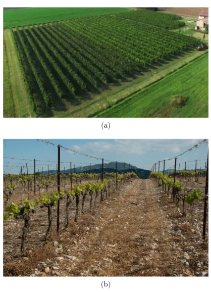
2.1 Dispenser shape and location . . . 6 2.2 Examples of a real vineyard and a rough terrain; (a) illustrates
a common Italian vineyard (b) shows the irregularity of the terrain . . . 8 2.3 Block diagram of sensor fusion and multi-sensor integration . . 11 2.4 the "Dassie" prototype . . . 15 2.5 Vinbot robot prototype . . . 16 2.6 Vinbot navigation architecture . . . 17 3.1 Illustration of importance resampling in particle filters: (a)
In-stead of sampling from f directly, we can only generate sam-ples from a different density, g. Samsam-ples drawn from g are shown at the bottom of this diagram. (b) A sample of f is obtained by attaching the weight f (x)/g(x) to each sample x. 27 3.2 ICC identification . . . 31 3.3 Example of differential drive robot . . . 32 3.4 Differential drive robot . . . 32 3.5 Differential drive robot motion from pose (x, y, θ) to (x′, y′, θ′) 34 3.6 Skid-Steering robot . . . 36 3.7 Skid-Steering and differential drive equivalence . . . 38 3.8 An instance of the pose tracking factor graph with four pose
vertices ΓWO(t) (circles), odometry edges eODO (triangles), two
shared calibration parameters vertices kθand kv(squares), two
GPS edges eGP S and the GPS displacement parameter S
(O)
GP S. . 43
3.9 ROAMFREE estimation schema. . . 45 4.1 GRAPE robot prototype . . . 57 4.2 ROS standard navigation stack . . . 58
4.4 Final navigation system architecture. Circles are nodes while rectangle are topics. The graph is simplified of some nodes or topics for clearness reason . . . 62 4.5 TF tree relative to the final architecture . . . 63 4.6 The hardware interface rosgraph. For clarity reasons some
driver nodes has been omitted . . . 64 4.7 Gazebo simulation node and its topics . . . 65 4.8 The sensor fusion and odometry estimation node in the two
variants. (a) shows our ROS implementation of ROAMFREE
(the raroam_node), (b) represents the nodes of robot_localization. 67 4.9 The SLAM_node in the three variants. (a) Gmapping, (b)
Google’s Cartographer, (c) KartoSLAM. . . 70 4.10 The autonomous navigation module . . . 71 5.1 The environment model simulated in Gazebo . . . 76 5.2 The difference between the accurate vine model (a) and
do-wnsampled model (b) . . . 77 5.3 TF tree of the simulation evaluation architecture . . . 79 5.4 Odometry estimator comparison. odom_r is the frame relative
to /raroam_node, odom_g is relative to /ekf_localization_gps and odom_f is relative to /ekf_localization_odom . . . 81 5.5 Map of the simulated vineyard, made with gmapping and ekf
(wheels+imu) odometry estimatot . . . 82 6.1 The MasLlunes vineyard. (a) is a satellite view, (b) shows the
vine lines and the ground . . . 85 6.2 Matlab viewer snapshot . . . 87 6.3 Maps of the MasLlunes vineyard built using robot_localization.
(a) KartoSLAM (Feb), completely wrong, (b) Google’s Carto-grapher (Feb), the map presents some erroneous lines in the lo-wer part, (c) Gmapping (Feb), acceptable map, even if slightly curve, but this usually does not interfere with the localization algorithm . . . 89
6.4 Maps of the MasLlunes vineyard built using ROAMFREE. (a) KartoSLAM (Feb), there are some inaccuracies and it is not acceptable without manual cleaning, (b) Google’s Cartogra-pher (Feb), it is a perfect map, (c) Gmapping (Feb), it is very good and straight . . . 90 6.5 Map of the MasLlunes vineyard in July, built using
ROAM-FREE and Gmapping . . . 93 6.6 Maps of the MasLlunes vineyard built using robot_localization.
(a) KartoSLAM (Feb), completely wrong, (b) Google’s Carto-grapher (Feb), the map presents some erroneous lines in the lo-wer part, (c) Gmapping (Feb), acceptable map, even if slightly curve . . . 94 6.7 Maps of the MasLlunes vineyard built using robot_localization.
(a) KartoSLAM (Feb), completely wrong, (b) Google’s Carto-grapher (Feb), the map presents some erroneous lines in the lo-wer part, (c) Gmapping (Feb), acceptable map, even if slightly curve . . . 95 C.1 A view of all the standard TF frames in Willow Garages PR2
Robot with the robot meshes rendered transparently and the edges of the tree hidden. The RGB cylinders represent the X, Y, and Z axes of the coordinate frames. . . 117
1.
Introduction
The application of autonomous robots in rough and unstructured environ-ments has increased exponentially over the last years, so that it has defined a new branch of robotics called field robotics. In particular one of the fields that is most developed recently is precision agriculture. Indeed in agricul-ture, robots are not only used for crop monitoring, like aerial inspection for growth control, but they are taking a key role in the daily life of farmers and producers. Heavy tasks like pruning, seeding or even precise harvesting are the target topics of these new robots.
The GRAPE project has born to accomplish one of these precision tasks: the distribution of pheromone for integrated pest control in vineyards. It is funded by Echord++ program from European Commission. This thesis carries out a specific part of the GRAPE project: the design of autono-mous navigation system of the GRAPE robot. In the title we defined it as “an experiment” since Echord++ uses this terms to define small-scale re-search projects with a maximum duration of 18 months aimed at verifying the readiness of a technology on the field
Autonomous outdoor navigation in a vineyard is a quite different pro-blem with respect to similar categories of propro-blems, like indoor navigation or autonomous on-road driving. Indeed outdoor scenarios contain some very important destabilizing factors which do not permit to use standard navi-gation methods as they are. Specifically, we can identify three main factors which are sources of variability: the soil, the weather and the vegetation. Each of these introduces noise in the data perceived from the robot sensors. For example the soil affects the mobility of the robot, and it is responsible for wheels slippage and robot platform wobbling. Such effects influences the perception done by the wheel encoders, by the IMU and by the LIDAR. The
weather, instead, alters the satellite reception and the quality of the LIDAR acquisitions. Finally the vegetation, depending on the season increase or de-crease the volume of the vines and the quantity of grass and weeds. This hinder the navigation of the robot in terms of number and size of obstacles.
1.1 Thesis contribution
To solve the variability of the vineyard environment this thesis proposes a multi-sensors navigation system that takes advantage of a robust sensor fu-sion framework, ROAMFREE, which provides tools to merge different sensors in the estimation of the odometry of a robot. The sensors merged are: wheel encoders, IMU and GPS.
Besides using GPS information the system performs the localization using two different approaches based on the task: if the task is the autonomous navigation the localization is done exploiting a particle filter in the form of Adaptive MonteCarlo Localization (AMCL) algorithm, otherwise if the task is to map the vineyard the localization takes places simultaneously with the mapping of the robot for the autonomous navigation task and exploits a technique, SLAM, able to build a map and simultaneously locate the robot in that map when the task is to map the vineyard. In both cases the robot acquires information about the obstacles and the environment structure using a LIDAR sensor.
The navigation system has been tested in a simulation environment crea-ted ad-hoc, which reproduces both the vine plants and the vineyard ground. We have obtained excellent results both in mapping and in autonomous na-vigation in this simulation environment. Afterwards the system has been installed and configured on a real robot, the GRAPE robot, which is a four wheeled skid-steering mobile robot based on the Husky platform.
The robot has been ran in a real vineyard to validate the performance of the navigation system in real case. During tests this latter has continuously provided the right localization of the robot. Further, the robot has been able to correctly map the vineyard and then to autonomously navigate using that map. For the mapping task the system has been tested with three different laser based SLAM tools: Gmapping, Google’s Cartographer and KartoSLAM. Gmapping outperformed the other approaches, since it proved to be more reliable in providing accurate maps.
Capitolo 1. Introduction 3
1.2 Structure of Thesis
The thesis is structured as follows.• In Chapter 2 we discuss and explain the challenges for autonomous
robot navigation due to the vineyard environment. In particular, we first introduce the GRAPE project context, in section 2.1, then we analyze the issues which are present in vineyard robot navigation and for which this thesis propose a solution, section 2.2. Finally we show other examples of vineyard robot in section 2.3
• In Chapter 3 we describe all the tools that we adopt in our solution and
the theoretical concepts to understand them. We start introducing the standard approaches for the state estimation in section 3.1. Then we explain the odometry estimation basics and we list the sensor fusion tools that we use to compute it, respectively in section 3.2 and in section 3.3. Finally we outline the most known methods for SLAM and for localization in section 3.4 and in section 3.5.
• In Chapter 4 we present the navigation system architecture we propose.
We first depict the final architecture, in section 4.2 and then we analyze singularly the sub-systems composing it from section 4.3 to section 4.7.
• In Chapter 5 we introduce the simulation environment in section 5.2
and then we describe and comment the simulation tests and results in the three tasks of odometry estimation and sensor fusion in section 5.3, mapping in section5.4 and autonomous navigation in section 5.5.
• In Chapter 6 we shows the vineyard used for validation tests in section
6.1 and we discuss the obtained results for mapping in section 6.2 and autonomous navigation in section 6.3.
• In Chapter 7 we summarize the obtained results and we propose some
possible futures improvements for the system.
• Appendix A introduces ROS, outlining its structure and its main
features.
• Appendix B reports the technical data about the sensor adopted for
Challenges in Field Robotics: the
vineyard case
In the Introduction we have mentioned some of the challenges that we faced during the thesis. In this chapter we first describe the GRAPE project and then we focus on the identification and explanation the problems due to the vineyard environment.
2.1 The GRAPE Project
The application of robotics as a support tool for farmers or automated sy-stems for agricultural tasks can offer the necessary step change in farming production in order to meet the future needs of an increasing world popula-tion, 34% by 2050 according to FAO1. GRAPE project aims at contributing to that technological breakthrough by developing a mobile robotic system endowed with a robotic arm able to perform precise agricultural tasks at plant level for vineyards.
GRAPE robotic concept is composed by four main technological compo-nents designed and integrated to monitor plants health in vineyards and to apply a biocontrol mechanism consisting of pheromone dispensers for plague control. These results will be validated in real scenarios covering a predefined range of scenarios in France, Italy and Spain, the three EU countries with the largest wine production.
The four technological components of the GRAPE projects are:
Capitolo 2. Challenges in Field Robotics: the vineyard case 5
• Vineyard navigation module based on advanced localization and
map-ping capabilities and path planning techniques considering terrain characteristics and kino-dynamic constraints to enhance safety and robustness.
• Plant health monitoring module implementing advanced perception
ca-pabilities for plant detection in highly unstructured and geometrically variable scenario and plant health assessment for early detection of problems.
• Precise manipulation and deployment for a targeted pheromone
dispenser distribution.
• User friendly operational interface enabling robot teleoperation, data
visualization and reporting.
A ground robot for plague control related tasks shall be able to navigate along the rows of vines typically found in this type of crops. The varie-ty of terrains and varie-typology of crops makes the definition of an application scenario extremely relevant for a correct requirements elicitation. This pro-ject belongs to Echord++ Program from European Commission. Vineyard protection becomes one of the main issues for the producers. Control of plagues, fungi and other threats are recurrent tasks in winery. This project is focused on the improvement of the plague control tasks, specifically on the installation of pheromone dispensers for matting disruption. The task of dispenser distribution is currently done manually where the operators walk through the vineyard hanging the dispensers in a regular distribution pattern (approximately one dispenser every 5-6 plants). There are different shapes available for the dispensers, depending on the brand, which is something to take into account for our manipulation developments. In our case, we use the dispensers provided by Biogard2, which is a reference company in Europe. Regarding the specific location to deploy the dispenser, it must be placed in one of the main branches. 2.1 shows the shape and the location of the phe-romone dispenser. The installation of dispensers should be performed early in the first moth flight (G1), which is to say from the end of March in the earliest areas until early April. In this period, the vineyard is just trimmed. This situation defines a particular scenario for dispenser deployment. The plants have no leaves and only the main branches (two horizontal) remain. The small branches are pruned. This particular situation have to be taken
Figura 2.1: Dispenser shape and location
into account in the use case development. The project is a collaboration bet-ween the Politecnico di Milano (Italy), the Eurecat research center (Spain) and Vitirover (France). The three entity should work on different task, in particular the Polimi team have to develop the navigation system and the manipulation part of the robot.
From a robotics perspective, there are two main aspects to take into account when analyzing the traversability challenges for a ground robot ope-rating in vineyards: slope of the ground and terrain morphology. Depending on the region, the vineyard distribution can be very challenging. Although the plant distribution is always in rows, the crop can be located in a plain terrain or in the mountainside. We identify three types of crops:
• Flat crops, located in an almost flat field maybe following the contour
of the hill but always in the same plane
• Hillside, with a slope less than 40% where the plants are organized in
rows with a horizontal path between them
• Mountainside, where plants are located in a hillside with more than
40% of slope. Usually, in best cases, there is a small path between rows, 60cm at most, which allows the operator walking through the crop, in order to do manual work. If not, there is no horizontal path and robotic deployment becomes almost impossible.
Another important aspect in the performance of a ground robot in a vineyard is the type of terrain. The performance of the robot largely depends on the
Capitolo 2. Challenges in Field Robotics: the vineyard case 7 type of soil. This can affect not only the navigation but also the battery consumption and motion control, among other aspects.
2.2 Robot navigation in vineyards
Field robotics is concerned with the automation of vehicles and platforms operating in harsh, unstructured environments. Field robotics encompas-ses the automation of many land, sea and air platforms in applications such as mining, cargo handling, agriculture, underwater exploration and exploitation, planetary exploration, coastal surveillance and rescue.
Field robotics is characterized by the application of the most advanced robotics principles in sensing, control, and reasoning in unstructured and unforgiving environments. The appeal of field robotics is that it is challenging science, involves the latest engineering and systems design principles, and offers the real prospect of robotic principles making a substantial economic and social contribution to many different application areas.
In general, field robots are mobile platforms that work outdoors, often producing forceful interactions with their environments and without human supervision. Many examples and other details about field robotics can be found at [1].
Field robotics is as much about engineering as it is about developing ba-sic technologies. While many of the methods employed derive from other robotics research areas, it is the application of these in large scale and de-manding applications which distinguishes what can currently be achieved in field robotics.
The autonomous navigation in a vineyard belongs to the category of the outdoor navigation that is one of the most challenging application of field robotics. In fact it has been described in many works already in the 90s. In particular there exists a work of Amit Singhal [2] that in 1997 identifies three main sub-problems relative to the unmanned outdoor navigation: the unstructured environments, moving obstacles and multiple sensors. Obviou-sly the moving obstacles and the multiple sensors are also problems for the indoor autonomous navigation but in a less accentuated manner. The majo-rity of the known techniques and algorithms in robotics are created for indoor scopes, thus adopting them for outdoor tasks is not simple and requires the usage some tricks since there are a lots of uncertainties and noise due to the environment.
(a)
(b)
Figura 2.2: Examples of a real vineyard and a rough terrain; (a) illustrates a common Italian vineyard (b) shows the irregularity of the terrain
2.2.1 Unstructured environments
For what concerns the unstructured environments, our robot has to work in vineyards that even if they are different in each geographical zone always maintain a similar skeleton: the vines are disposed in straight lines that have a fixed separation distance among them, the vines belonging to the same line are equidistant and often, in a vineyard, there are chunks of lines that share the same length. Some examples of real vineyards can be seen in the 2.2. Thus, we dont have a lack of structure, but we must note that the described structure is very repetitive and this represent a drawback especially during
Capitolo 2. Challenges in Field Robotics: the vineyard case 9 navigation tasks. In fact, its harder for the robot to localize itself in points of the vineyard which are very similar to others. Furthermore, if on one hand we have an almost fixed structure on the other we have the presence of some instability factors such as the ground, the weather and the vegetative state of the environment. The ground problem is one of the most difficult to solve due to its high variability. Indeed, the terrain is bumpy (see Figure 2.2b) and its consistency changes based on the geolocation and the weather so it affects always differently the movements of the robot. In particular it influences the slippage of the wheels, that increases the unreliability of the wheel encoders acquisitions and it makes the robot platform wobble that increments the noise of the measurements coming from the sensors fixed on it (except for the GNSS). The vegetative state of the environment changes with the seasons and can completely transform the aspect of it. During the late autumn and the winter, the nature is bare, the vine plants havent leaves and the ground has few grass and weeds. Instead during the others months, the surroundings are green, so the vines are full of leaves and in certain periods are also full of grapes while the terrain presents a lot of grass. Obviously in this period many maintenances are done to make the vineyard clean and to permit to work in it, but often the result is approximately clean and so many obstacles remain. The problem created by the vegetation of the vineyard its a visibility problem for the robot. In fact, the presence of leaves and weeds near the plants increases the size of the obstacles and make them less definite (its harder to identify the single vines) to the robots eyes. Furthermore, if there are some high weeds (at least as high as the LIDAR sensor level), they become new obstacles for the robot and makes the autonomous navigation more difficult (they mislead the planner when it draws the path). Finally, the weather impact is the more relative, since obviously the robot is expected to work with acceptable atmospheric conditions, thus no rainfall and not too much wind. Nevertheless, the weather, also when it is acceptable, can influence the satellite reception or the LIDARs acquisitions quality, thus in general the accuracy of the sensors.
2.2.2 Moving obstacles
Then we talk about the presence of moving obstacles and it is clear that in our case this problem is the one that is the most similar to indoor navigation. For many unmanned outdoor robots, the scenario is completely different
from our one, i.e. autonomous cars, and the moving obstacles represent a very sensitive issue. However, in all scenarios the problem is faced with robust and, sometimes complex, local planner, thus planning algorithm that are designed to reacts in real time to unexpected changes. Thinking to our scenario there are moving obstacles when it happens that a living being hinds the path that the robot is following. This is a quite rare case in a vineyard since it doesnt guest much animals and humans are not expected to be present in front of the robot while it runs. These kind of events are even more probable in an indoor scenario. What can happen in our case is that the atmospheric conditions create some new unexpected obstacles, i.e. the wind can carry some small objects.
2.2.3 Multiple sensors
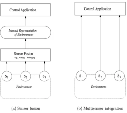
Finally, the multiple sensors problem. First of all, we have to make a brief explanation of what we mean when we talk about this problem. In fact, in the literature there exists a clear distinction between multi-sensor integration and sensor fusion. The differences between these two has been well explained in a work of Wilfried Elmenreich [3] and we summarize it here in the 2.3.
In our work we will always refers to sensor fusion and for this reason we report the definition given by Elmenreich. Sensor Fusion is the combining of sensory data or data derived from sensory data such that the resulting in-formation is in some sense better than would be possible when these sources were used individually. Another definition of sensor fusion can be found in the article of Kam et al. [4], but its more mathematical and so we prefer to not bring it here. Now that we have a definition, we can start explaining why the sensor fusion problem is adapt to our scenario and what are the issues in it. Looking at the definition of Elemenreich is simple to understand that sensor fusion is needed to improve the accuracy of the state estimation of a robot. In fact, the simultaneous usage of multiple sensors allows the robot to have a more complete knowledge of the environment and so it enriches its internal world representation. Robots differently from humans dont need a global vision of the surrounding environment, but they need the informa-tion necessary to complete the tasks for which they are designed. Thus, it is important to choose the right sensors to collect only interesting data (we explain our choices in the chapter 4), in the case of mobile unmanned navi-gation and especially in our case is fundamental to have more sensors. There
Capitolo 2. Challenges in Field Robotics: the vineyard case 11
Figura 2.3: Block diagram of sensor fusion and multi-sensor integration
are many reasons of this need and some of them can be retrieved in the problems that we already described. We can say that the multiple sensors problem is, in part, a consequence of the other two, since it belongs to the solutions of them. Thus, solving this problem means also to solve a portion of the others. In general, the advantages that sensor fusion can leads to are the following:
• Robustness and reliability: Multiple sensor suites have an inherent
re-dundancy which enables the system to provide information even in case of partial failure.
• Extended spatial and temporal coverage: One sensor can look where
others cannot respectively can perform a measurement while others cannot.
• Increased confidence: A measurement of one sensor is confirmed by
measurements of other sensors covering the same domain.
• Reduced ambiguity and uncertainty: Joint information reduces the set
• Robustness against interference: By increasing the dimensionality of
the measurement space (e.g., measuring the desired quantity with op-tical sensors and ultrasonic sensors) the system becomes less vulnerable against interference.
• Improved resolution: When multiple independent measurements of the
same property are fused, the resolution of the resulting value is better than a single sensors measurement.
There exist many methods that face the sensor fusion problem and based on the approach they give a different mathematical definition of the problem. Among all the approaches there are three types that have been mostly used in the last few years, thanks to their performance and reliability. These are two Bayesian approaches: one Gaussian, the Kalman filter and one non-parametric, the Particle filter; and the graph-based approach. In our work we will test all these and in the end we will combine two of them in our proposed solution. The differences between these types of state estimation techniques and their description is explained in chapter 3 3. After this brief digression on the possible solutions to the sensor fusion problem, we can resume explaining what are the intrinsic issues of using more sensors. A first and basic consideration is that every real sensor is affected by some noise, so it provides measurements containing an error. Usually this error is composed by two parts: one expected and one unexpected or unpredictable, using more technical words they are, respectively, the statistical bias and the standard deviation. For all commercial sensors there exists a descriptive data-sheet in which the value of the expected error is specified, since its an error that is intrinsic of the sensor for construction reasons. Thus, the knowledge of the bias can be exploited, with a simple post processing, to have better measurements in the state estimation. Instead, it remains unknown the unexpected part of the error since its dependent from external factors, in our case the ones coming from the outdoor environment, and thus it has to be identified and reduced in real-time. In order to notice the entity of the unexpected error is fundamental to have more sources of data which provide an inherent measurement, thus more sensors collecting information on the same domain, but from a different point of view. Its consequent that the redundancy is a very important feature for sensor fusion, obviously in the convenience limits. In fact, Its implicit that it is not meaningful to have too much sensors measuring the same variable both for the economic side and for
Capitolo 2. Challenges in Field Robotics: the vineyard case 13 the computational complexity side. Integrate and merge acquisitions coming from different sources is a very hard work since all the differences have to be uniformed. What changes between the various sensor is: the frequency with which they acquire data, the unit of measure and their uncertainty. The amount of uncertainty is the most influent factor for the greatness of a sensor fusion system, indeed there exists a well-known work of Fowler [5] in which he comments the military systems and in particular he spends some words about the usage of multiple sensors. He says: Massaging a lot of crummy data doesnt produce good data; it just requires a lot of extra equipment and may even reduce the quality of the output by introducing time delays and/or unwarranted confidence. Thus, it is fundamental to have sensors that provide good quality data and for this aim it is often necessary to calibrate them before start executing the desired tasks. The importance of the calibration phase should not be underestimated, especially for certain type of sensors which otherwise produce harmful data. In case where its not possible to successfully complete this phase it is better to discard at all the information coming from the interested sensors.
In outdoor environments the sensors used for the planar navigation must be able to perceive the robot movements and the obstacles. The clearer is the data acquired the simpler is the localization and thus the navigation of the robot. For these reasons the sensors, usually, adopted are: GPS, wheel encoders, IMU (gyroscope, magnetometer, accelerometer) and laser range finders. The GPS sensor is very important for outdoor robot, it allows to have a real geolocation and thanks to the the last year improvement it is also able to provide precise measure through the RTK adjustments. The curse of the GPS is always the unreliability since it depends from the satellite reception. So, building systems that are heavily based on the GPS work is never a good choice, even in case like our one in which there is no signal reflection problem and there are not very high barriers. Furthermore, the GPS (without RTK correction) also suffers of multiple paths problem, thus in the vineyard it can leads to jump among different lines. The wheel encoders are really precise in the measurements, since they are internal sensor, but the problem here is, as we stated above, the wheels slippage. This latter has a different influence depending on the kinematic model of the robot (wheels disposition). The gyroscope and the accelerometer are highly influenced by the robot stresses due to the irregularity in the terrain. The magnetometer is a very delicate sensors, in the sense that it is really sensitive to more factors:
the geolocation, the presence of magnetic distortion due to metals or cables around it. Finally the LIDAR is often quite stable, but it is measurement depends on the robot platform inclination and thus it is influenced by the rough ground. Further it has also some influence by the weather that we already cited.
2.2.4 Simulation problems
Simulation is the imitation of the operation of a real-world process or system over time; in robotics it corresponds to a software able to reproduce as real as possible the robot and its working environment. This means to reproduce all the physical behaviors of each component of the desired world and in par-ticular of the robot model. Furthermore, thanks to the growing technologies in computer graphics, the simulators are also able to show graphically what is happening during the tests.
On the other hand, reproducing graphically and physically an entire en-vironment is a very complex operation and thus the simulator results to be a very heavy software respect to the computational power of common PCs. The weight of a simulation depends on the quantity and the quality of the objects that have to be reproduced and based on these values the simulation is more or less flowing.
In our thesis we need to simulate both the vineyard and the GRAPE robot. In particular the simulation of the vineyard is not a simple task due to its high variability. Indeed the terrain and the plants have not a constant shape, thus reproducing them with a 3D model introduces a relevant approximation error. In addition, it is not possible to reproduce the weather condition which another variability factor of the environment. We can assert that, the simulated environment is always a simpler approximation of the reality and in this scenario the approximation is even higher with respect to other scenarios. Despite these approximations the models representing the outdoor environment are very complex, both physically and graphically, thus they can lead to some fluency problem during the simulation or to inconsistency problem (if the physical model has some lacks).
Capitolo 2. Challenges in Field Robotics: the vineyard case 15
Figura 2.4: the "Dassie" prototype
2.3 Other similar projects
In the last years in the agricultural robotics is rapidly increasing the number of unmanned robots. We report here some examples of other projects that like our one have to deal with the field robotics problem. In particular we describe robots that has been developed for the vineyard work. Almost all are not already in commerce and in general we don’t have access to much information about their navigation systems.
The first example of a similar robot is the one developed in SouthAfrica by a collaboration between the CSIR (Council for Scientific and Industrial Research) and the Stellenbosch University. The aim of this project is to create a cost-effective platform to inspect and monitor horticultural crops on local farms. The robot prototype is called Dassie 2.4, is quite agile and can easily move around in the vineyard. A few sensors have been fixed to the platform and include a laser (LIDAR) scanner as well as high definition cameras facing to the front and sideways. The robot can also pull an electro-magnetic induction sensor behind it to be able to map soil differences. All measurements that it acquire are streamed to an online computer able to pro-cess the information. After the prototype development it has been tested in a vineyard and thus the sensors have been configured to estimate grape yield
Figura 2.5: Vinbot robot prototype
and to monitor plant growth and canopy health. Currently, it is able to navi-gate autonomously through the vineyard, using CSIR-developed data-sensor fusion techniques to combine the data from the different sensors. Using the CSIR-designed data-fusion algorithm, it is also able to perform path plan-ning, obstacle avoidance and lane following. Unfortunately we don’t have information about the sensor fusion algorithm and the navigation system structure, thus we cannot compare our intuitions with their ones.
The second example that we report is another vineyard robot built under an European project: VinBot.
The VinBot project is a European project: "Autonomous cloud-computing vineyard robot to optimise yield management and wine quality" in which there is an all-terrain robot that monitors vineyard criteria essen-tial to successful yield management by accurately estimating, by means of computer vision: the quantity of leaves, the quantity of fruit and the grapes exact location on the vine.
The VinBot consists of an autonomous wheeled mobile robot based on the Robotnik platform Summit XL HL. See Figure 2.5.
It mounts:
Capitolo 2. Challenges in Field Robotics: the vineyard case 17
Figura 2.6: Vinbot navigation architecture
• a RTK-DGPS antenna for high accuracy geo-localization
• two lasers Hokuyo 30m outdoor sensors (one for navigation purposes,
the second for plant 3d scanning)
• a small computer for basic computational functions running ROS • a dual interface communication system using Wi-Fi and Radio
Looking at the navigation system it proposes an hybrid reactive/waypoint based navigation architecture. It makes use of a laser range finder and RGBD device to perform reactive row following and obstacle avoidance, while it can make use of other reactive behaviors or GPS waypoint navigation for changing from row to row or field to field, thus supporting different levels of automation. In particular the hybrid architecture implements a high level planner able to receive and store a sequence of waypoints or reactive actions from an external HMI (Human Machine Interface). The reactive actions are preset and are: follow the right/left row, follow the 2 rows (center), turn to the right/left row, turn in-site 180o. The planner is implemented through ROS actionlib stack and provides the waypoints and the reactive actions through two different action servers. The structure is described in 2.5. Then, the VinBot proposal implements the localization of the robot through the ROS package robot_localization, that we will explain the next chapter. Thanks to this package they obtain a localization by merging the
wheel odometry the IMU measurements and the GPS data. They show and discuss their navigation results in this paper [6].
In the chapter 4 we illustrate our navigation system, there it can be observed the different choice respect to the VinBot solution.
3.
Relevant background and tools
In this chapter we describe as clearer as possible the methods that we will exploit in our solution and the theoretical background necessary to under-stand them. Since this thesis belongs to an applicative field such as the field robotics in which there is an infinite quantity of different scenarios, we don’t have a pure state of the art, but we have a set of tools that are currently adopted in the majority of the cases (similar to our one) and that for the specific task that each of them solve, they are one of the most known solu-tions. Thus, we will present them through their real implementation in order to be specific in preparation to the next chapters. Going in a logic sequence, we analyze as first the techniques that face the odometry estimation with the sensor fusion, describing the robot_localization implementation and the ROAMFREE framework. Then, we illustrate the methods able to solve the SLAM problem referring in particular to Gmapping implementation, but also mentioning different approaches such as KartoSLAM and Google’s Cartogra-pher. Finally, we describe the localization approach explaining the most used algorithm and tool, AMCL.
3.1 Background
Since the tools that we report have shown great performance in solving diffe-rent and difficult applied problems, the background that stays behind them is almost a state of the art for mobile robot navigation. In fact, we explain the concept of state estimation and consequently the various approaches which try to solve it that have emerged in the recent years, such as the Kalman filters, the particle filters and the graph-based filters.
3.1.1 State estimation
In the previous chapter we analyzed the general problems of the outdoor un-manned navigation adapting some of them to our specific case. In particular we showed how the problems relative to multiple sensors are very important in our case and influence the state estimation. Now we go one step further by describing with more details the whole state estimation since it is funda-mental in order to make the robot navigate autonomously. We describe the state estimation as the ensemble of two parts: the first regards the odometry estimation while the second depends on the aim of the robot, that in our case can be the mapping of the environment or the localization for the na-vigation in a known map. These two parts are strictly linked, in particular the second needs the first. Technically speaking the sensor fusion is present in both the parts, but in two different ways. In fact, in the first part all the sensors that give information about the movement of the robot are taken into account, thus wheel encoders, gyroscope, gps etc., instead in the second part the merging is between the estimated odometry and the laser acquisi-tions. If the estimated odometry is erroneous the second part has a more difficult work and very often, if not always, this means to have worst results. Thus, the odometry estimation is crucial in order to obtain good results, in our case this means accurate maps and a precise localization. Furthermore, the complex is the scenario the higher is the importance of the estimated odometry.
In the previous chapter we outlined the existence of three types of ap-proaches for the state estimation, these are the one representing the basis for the methods that solve the two parts that we just mentioned. Thus, be-fore explaining these methods we illustrate the basic concepts of the three approaches.
3.1.2 Bayesian approaches
The Bayesian approaches are the first important category for the theory of the state estimation in robotics. Obviously, they make usage of the Bayes statistic principles that can be found in chapter 2 of the this book [7]. In general all the approaches belonging to this category start their reasoning from the belief definition. The belief is the posterior of the state and thus is defined by the formula
Capitolo 3. Relevant background and tools 21 This posterior is the probability distribution over the state xt at time t,
conditioned on all past measurements z1:t (sensor acquisitions) and all past
controls u1:t (robot control inputs). This definition include also the
measure-ment zt, but it is not always convenient to wait for this measurement before
estimate the state, thus there exists another definition of the belief
bel(xt) = p(xt|z1:t−1, u1:t) (3.2)
In the probabilistic filtering this distribution is called prediction, due to the fact that bel(xt) predicts the state at time t based on the previous state
posterior before incorporating the measurement at time t. Starting from this definition we can obtain the bel(xt) by applying a step, known as correction
or measurement update. Bayes filter
The first type of filter we analyze is the most simple, the Bayes filter. It com-putes the belief in a recursive way, thus the bel(xt) is computed using bel(xt−1)
along with the most recent control ut and the most recent measurement zt, bel(xt) = ηp(zt|xt)
∫
p(xt|ut, xt−1)bel(xt−1)dxt−1 (3.3)
where η is a normalization term. This equation can be obtained starting from (3.1) thanks to the Bayes rule and two assumptions: (i)the states follow a first-order Markov process, p(xt|x0:t−1) = p(xt|xn−1); (ii)the observations are
independent of the given states, i.e. p(zt|x0:t, z1:t, u1:t) = p(zt|xt).
The filter can be described more clearly through the pseudo-algorithm reported below. It can be observed that it is composed of two steps, the pre-diction and the correction. In the prepre-diction bel(xt) is computed integrating
the prior belief over state xt−1, and the probability that control ut induces
a transition from xt−1 to xt. Instead in the correction or update step the bel(xt) just computed is multiplied by the probability the measurement zt
may have been observed and since this product can result greater than 1, it is normalized with the parameter η. The initialization of the belief, bel(x0),
is necessary to make the algorithm start and it can be done with certainty if it that value is known or it can be generated with a uniform distribution (or a different one) if it is unknown (or partially known).
The problem of this algorithm is the complexity, in fact the presence of an integral is a bottleneck and further the product in the update state can
Algorithm 1 Bayesian filtering function BayesFilter(bel(xt−1), ut, zt) for all x do bel(xt)← ∫ p(xt|ut, xt−1)bel(xt−1)dx bel(xt)← ηp(zt|xt)bel(xt) end for return bel(xt) end function
Algorithm 2 Kalman filtering
function KalmanFilter(µt−1, Σt−1, ut, zt) µt← Atµt+ Btut Σt← AtΣt−1ATt + Rt Kt← ΣtCtT ( CtΣtCtT + Qt )−1 µt← µt+ Kt(zt− Ctµt) Σt← (I − KtHt) Σt return µt, Σt end function
result very complex. Thus, a classical Bayes filter can be used only for very simple problems in which the state space is very limited, since in these cases the integral can be reduced to a finite sum.
Kalman filter
The Kalman filter (KF) is the first practical implementation of the Bayes filter. It was invented by Rudolph E. Kalman in the 1960. It try to transform the bayesian filter formulation in a efficient one, deleting the integral and putting it in a closed form. To do this, It assumes the beliefs are Gaussian: At time t, the belief is represented by the the mean µt and the covariance
Σt. In addition to the Markov assumptions there are other three properties
that are needed to treat the beliefs as Gaussian: (i) the states are linear,
xt = Atxt−1 + Btut + ϵt where At and Bt are matrices having dimension
according to the ones of the state vector xt and control vector ut, while ϵ is a
Gaussian noise; (ii) the measurement probability is linear in its arguments,
zt = Ctxt + δt, where Ct is matrix and δ a Gaussian noise; (iii) bel(x0) is
Capitolo 3. Relevant background and tools 23 Algorithm 3 Extended Kalman filtering
function ExtendedKalmanFilter(µt−1, Σt−1, ut, zt) µt← g(ut, µt−1) Σt← GtΣt−1GTt + Rt Kt← ΣtHtT ( HtΣtHtT + Qt )−1 µt← µt+ Kt(zt− h(µt) Σt← (I − KtCt) Σt return µt, Σt end function
Given all the assumptions the Kalman filter can be formulated in a clo-sed form that we report with a pseudo algorithm. The demonstration of the listed formulae can be found at [7]. Again we have a two steps filter. The differences respect to the purely Bayes filter are that the beliefs are substi-tuted by the mean, µt, and the covariance Σt that are predicted in the first
two lines by including the new control utand updated in the remaining ones
by considering the new measurement zt. Another news is represented by the
variable Kt that is known as Kalman gain and specifies the degree to which
the measurement is incorporated into the new state estimate.
Thanks to its matrix formulation the Kalman filter can be solved in a closed form and thus results efficient. Instead, it suffers for what concern the generality, in the sense that very often the assumptions (i) and (ii) are too strong, thus far from the reality and so it cannot be applied in many real cases. For this reason it has been evolved to an Extended version, so EKF. Extended Kalman Filter
The EKF solve the problems of the KF by replacing the linear predictions with their nonlinear generalizations. Moreover, EKFs use Jacobians Gt and Ht instead of the corresponding linear system matrices At, Bt, and Ct in
Kalman filters. The Jacobian Gt corresponds to the matrices At and Bt,
and the Jacobian Ht corresponds to Ct. Thus it maintain the computational
efficiency and the simplicity of the KF while it adds the applicability to many cases, it results robust also in for unexpected problems (problems that violate the underlying assumptions). We report here the pseudo algorithm, just for simplify the comparison with the standard KLF, but we then explain all the passages in section 3.3.1 where it has a real implementation.
The EKF main limit is that it approximates state transitions and measu-rements using linear Taylor expansions [8] . In virtually all robotics problems, these functions are nonlinear. The goodness of this approximation depends on two main factors. First, it depends on the degree of nonlinearity of the functions that are being approximated. If these functions are approximately linear, the EKF approximation may generally be a good one, and EKFs may approximate the posterior belief with sufficient accuracy. However, someti-mes, the functions are not only nonlinear, but are also multi-modal, in which case the linearization may be a poor approximation. The goodness of the linearization also depends on the degree of uncertainty. The less certain the robot, the wider its Gaussian belief, and the more it is affected by nonlinea-rities in the state transition and measurement functions. In practice, when applying EKFs it is therefore important to keep the uncertainty of the state estimate small. We also note that Taylor series expansion is only one way to linearize. In fact, there exist other two approaches that have demonstra-ted to lead to better results. One is the Unscendemonstra-ted Kalman filter (UKF), which probes the function to be linearized at selected points and calculates a linearized approximation based on the outcomes of these probes. Another is known as moments matching, in which the linearization is calculated in a way that preserves the true mean and the true covariance of the posterior distribution (which is not the case for EKFs).
Particle filter
An alternative to the Kalman filters (in general to Gaussian filters) are non-parametric filters. These filters do not rely on a fixed functional form of the posterior, such as Gaussians. Instead, they approximate posteriors by a finite number of values that are samples of the real distribution (state space). The number of parameters used to approximate the posterior can be varied. The quality of the approximation depends on the number of parameters used to represent the posterior. As the number of parameters goes to infinity, non-parametric techniques tend to converge uniformly to the correct posterior (under specific smoothness assumptions). Some nonparametric Bayes filters rely on a decomposition of the state space, in which each such value corre-sponds to the cumulative probability of the posterior density in a compact subregion of the state space. Others approximate the state space by random samples drawn from the posterior distribution. In particular, we explain a
Capitolo 3. Relevant background and tools 25 method belonging to this latter category, called particle filter.
The particle filter is a nonparametric implementation of the Bayes filter, thus it start from the same belief definition, but it approximate the posterior distribution by using a finite number of parameters, the particles. The key idea of the particle filter is to represent the posterior bel(xt) by a set of
random state samples drawn from this posterior. 3.1 illustrates this idea. Obviously, this representation is an approximation of the real distribution, but being drawn from the posterior it is able to represent a much broader space of distributions.
The particles are denoted as
Xt = x (1) t , x (2) t , ..., x (M ) t
where M is the finite number of particles (usually large). Each particle x(m)t (with 1 ≤ m ≤ M ) is a concrete instantiation of the state at time t, thus it is a hypothesis about what the true world state may be at time t. In some implementations M is a function of t or of other quantities related to the belief. Thus the belief bel(xt) is approximated by the set of particles Xt.
Ideally, the likelihood for a state hypothesis xt to be included in the particle
setXt shall be proportional to its Bayes filter posterior bel(xt):
x(m)t ∼ p(xt|z1:t, u1:t) (3.4)
As a consequence of (4.23), the denser a subregion of the state space is populated by samples, the more likely it is that the true state falls into this region. This property should hold only for M → ∞, but in practice this can approximated drawing the particles from a slightly different distribution and using a not too small M (i.e. M ≥ 100).
Just like all other Bayes filter algorithms, the particle filter algorithm constructs the belief bel(xt) recursively from the belief bel(xt−1) one time
step earlier. Since beliefs are represented by sets of particles, this means that particle filters construct the particle set Xt recursively from the set Xt−1. The most basic variant of the particle filter algorithm is shown in
the Algorithm 4. The input of the algorithm are the particles Xt−1, the
most recent control ut and measurement zt. In the first cycle the algorithm
constructs the temporary set X which is reminiscent (but not equivalent) to belt. In this cycle the first step generates a hypothetical state x(tm) for
time t based on the particle x(t−1m) and the control ut. The m apex of the
Algorithm 4 Particle filtering function ParticleFilter(Xt−1, ut, zt) Xt← Xt← ∅ for all m := 1 to M do sample x(m)t ∼ p(xt|ut, x(m)t−1) wt(m)← p(zt|x (m) t ) Xt← Xt+⟨x (m) t , w (m) t ⟩ end for for all m := 1 to M do
draw i with probability∝ w(i)t add x(i)t to Xt
end for return Xt
end function
sampling is done from the distribution p(xt|ut, x
(m)
t−1). Then the second step
calculates for each particle x(m)t its importance factor (weight) wt(m), which is the probability of zt under the particle x
(m)
t . Finally the third step adds
iteratively the new samples with the correspondent weights to the set X . In the second cycle the algorithm implements the resampling or impor-tance resampling. Thus it draws with replacement M particles from the temporary set Xt. The probability of drawing each particle is given by its
importance weight. Resampling transforms a particle set of M particles in-to another particle set of the same size. By incorporating the importance weights into the resampling process, the distribution of the particles chan-ge: whereas before the resampling step, they were distributed according to
bel(xt), after the resampling they are distributed (approximately) according
to the posterior bel(xt) = ηp(zt|x
(m)
t )bel(xt). In fact, the resulting sample set
usually possesses many duplicates, since particles are drawn with replace-ment and the particles that are not contained in it tend to be the ones with lower importance weights.
The importance resampling is the main feature of the particle filters, in fact it allows to draw particles from a known distribution, called proposal distribution, and iteratively update them according to their relative weights until the set of sample approximate enough correctly the target distribution,
Capitolo 3. Relevant background and tools 27
(a)
(b)
Figura 3.1: Illustration of importance resampling in particle filters: (a) Instead of sampling from f directly, we can only generate samples from a different density, g. Samples drawn from g are shown at the bottom of this diagram. (b) A sample of f is obtained by attaching the weight f (x)/g(x) to each sample x.
and the target function computed in it. Thus
w(m)t = f (x
(m)
t )
g(x(m)t ) (3.5)
where f is the target distribution and g is the proposal one. The resampling step is easily synthesized in the Figure (3.1).
The approximation errors in particle filters are unavoidable since the set of sample is a discrete distribution while the target distribution is a continuos one. In particular, there are four complimentary sources of approximation error, each of which gives rise to improved versions of the particle filter.
1. The first approximation error relates to the fact that only a finite num-ber of particles are used. This introduces a systematic bias in the posterior estimate. Thus, it is fundamental to use an high number of particles M in order to limit the degree of approximation.
2. A second source of error in the particle filter relates to the randomness introduced in the resampling phase. In particular, the resampling pro-cess induces a loss of diversity in the particle population, which in fact manifests itself as approximation error. Such error is called variance of the estimator: Even though the variance of the particle set itself decreases, the variance of the particle set as an estimator of the true belief increases. Controlling this variance, or error, of the particle filter is essential for any practical implementation.
3. A third source of error pertains to the divergence of the proposal and target distribution. In fact, the more they are different the more the algorithm must iterate to approximate the target. Thus, the efficiency of the particle filter relies crucially on the match between the proposal and the target distribution. If, at one extreme, the sensors of the robot are highly inaccurate but its motion is very accurate, the target distri-bution will be similar to the proposal distridistri-bution and the particle filter will be efficient. If, on the other hand, the sensors are highly accurate but the motion is not, these distributions can deviate substantially and the resulting particle filter can become arbitrarily inefficient.
4. A fourth and final disadvantage of the particle filter is known as the particle deprivation problem. When performing estimation in a high-dimensional space, there may be no particles in the vicinity to the correct state. This might happen because the number of particles is too small to cover all relevant regions with high likelihood, but it is not the only reason. In fact, also for M enough high during the resampling there is a probability greater than zero (due to the random nature) that all the particles near the true state are wiped out.
Capitolo 3. Relevant background and tools 29 In conclusion the particle filters performance strongly depends on the number of particles used, that obviously is very difficult to be pre-estimated. Thus, it is usually tuned during the experiments. In particular, the complex is the state space the higher should be the number of particles.
3.1.3 Graph-based approaches
The development of graph-based approach in robotics starts in 1997 when Lu and Milios [9] propose a graph-based solution to the SLAM problem. In fact, in the recent years graph-based has been heavily applied to the SLAM problem since it allows to formulate the problem in a very intuitive way. As we will see better in the SLAM section, 3.4, the basic formulation using a graph represent the robot poses as nodes while the landmark parametri-zation builds the edge. Thus, if a landmark is visible from a certain pose, then an edge is added between the two poses. The state estimation problem is then formulated as a max-likelihood optimization over the built graph in which the goal is to find the configuration of robot poses and landmarks such that the joint likelihood of all the observations is maximum. The graph structure allows to exploits many statistical tricks, especially regarding the joint probabilities since the nodes connections impose the dependency and independency of the variables. Common statistical graph based approaches are the Bayesian networks (belief networks), the Markov networks and many others [10]. The graph state estimation to be solved requires a large non-linear, least-squares, optimization problem. For this reason the greatness of the optimization method is very important for the efficiency and the ap-plication of a graph-based algorithm. In fact, Graph-based approaches are nowadays considered superior to conventional Bayesian solutions [11] , but they needed some major advancements in sparse linear algebra [12] to beco-me competitive from the point of view of computational complexity. For a modern synthesis of these optimization methods see [13].
The advent of graph techniques in SLAM slightly changed the perspective from the state estimation point of view: while filters typically model state estimation as a recursive process performed measurement-per-measurement and the state consists of the latest robot pose and all the landmarks, graph-based approaches attempt to estimate the full robot trajectory, and thus a (long) sequence of robot poses together with the landmark positions form the whole set of measurements. This notion was already present in other
approaches [14] which never found a robotics application due to the counter intuitive structure. From the SLAM formulation the graph approach has been generalized even further, considering hyper-graphs, called factor graphs [15] that allows a more flexible graph building. We illustrate them in section 3.3.2. Thanks to this very generic graph many powerful tool for multi-sensor fusion has been developed [16]. In particular we will explain in details a tool called ROAMFREE that will solve for us the sensor fusion problem.
3.2 Odometry estimation
We just wrote about the importance of odometry estimation in complex scenarios, thus also in our one. The odometryăis the use of data fromămotion sensorsăto estimate change in position over time. It follows that the goal of the odometry estimation is to estimate as well as possible the pose (position and orientation) of the robot given the sensor acquisitions and the initial pose of the robot in a certain time interval.
3.2.1 Odometry
The simplest method to compute the odometry is only numeric. The stan-dard odometry estimates the distance travelled by measuring how much the wheels have turned, thus it integrates the velocity measurements over the time. The computation differs according to the number and the shape of wheels mounted on the robot. The simplest case is a single freely rotating wheel that, if considered with ideal conditions, implies to cover a distance on the ground of 2πr for each rotation, where r is the radius of the wheel. In practice, even the behavior of a single wheel is substantially more com-plicated than this. In fact, there are many variable factors that can create error, such as the wheels that are not necessarily mounted so as to be per-pendicular, nor are they aligned with the normal straight-ahead direction of the vehicle. In addition to these issues related to precise wheel orientation and lateral slip, there can also be insufficient traction that leads to slipping or sliding in the direction of the wheels motion, which makes the estimate of the distance travelled imprecise. Then other factors arise due to compaction of the terrain and cohesion between the surface and the wheel (as we stated in Chapter 2).
Capitolo 3. Relevant background and tools 31
Figura 3.2: ICC identification
Each wheeled mobile robot (WMR) to be able to move must have a point around which all wheels follow a circular course. This point is known as the instantaneous center of curvature (ICC) or the instantaneous center of rotation (ICR). In practice it is quite simple to identify the ICC because it must lie on a line coincident with the roll axis of each wheel that is in contact with the ground, see Figure 3.2. Thus, when a robot turns the orientation of the wheels must be consistent and a ICC must be present otherwise the robot cannot move.
A WMR can only moves on a plane and thus it has three degrees of freedom represented by the three component of the pose (x, y, θ) where (x, y) is the position and θ is the heading or orientation. The ability to have complete independent control over all these three parameters depends on the disposition and the number of wheels and usually mobile robots dont have a complete control. Thus, they are obliged to perform complex maneuvers in order to reach a desired pose (i.e. car parking). Referring to our case, we now describe the type of kinematic of our robot, in order to understand what are the motion that it can or it cannot do. Our robot moves with a skid-steering kinematic that is a derivative of the differential drive kinematic. 3.2.2 Differential drive odometry
Differential drive is probably the simplest possible drive mechanism for a ground contact mobile robot. Often used on small, low-cost, indoor robots such as the TurtleBot [17] or Khepera [18], larger commercial bases such as the Robuter [19] utilize this technology as well. As depicted in Figure 3.3 , a differential drive robot consists of two wheels mounted on a common axis, thus parallel, controlled by separate motors.
Figura 3.3: Example of differential drive robot
Figura 3.4: Differential drive robot
Consider how the controlling wheel velocities determine the vehicles mo-tion. For each of the two drive wheels to exhibit rolling motion, the robot must rotate around a point that lies on the common axis of the two drive wheels. By varying the relative velocity of the two wheels, the point of this rotation can be varied and different vehicle trajectories chosen.
At each instant in time, the point at which the robot rotates must have the property that the left and right wheels follow a path that moves around the ICC at the same angular rate ω, and thus
ω(R + l/2) = vr ω(R− l/2) = vl,
where l is the distance along the axle between the centers of the two wheels, the left wheel moves with velocity vl along the ground and the right with
velocity vr , and R is the signed distance from the ICC to the midpoint