Variational Multi-Scale Large Eddy simulations of the flow around a 5:1 rectangular cylinder

(1)

Universit´

a di Pisa

Facolt´

a di Ingegneria

Tesi di Laurea Specialistica in

Ingegneria Aerospaziale

Variational Multi-Scale Large Eddy

simulations of the flow around a 5:1

rectangular cylinder

Candidato: Valeria Angelino

Relatori: Prof.ssa Maria Vittoria Salvetti Dr. Ing. Annabella Nicoleta Grozescu

(2)

”Je crois que si l’on regardait toujours les cieux, on finirait par avoir des ailes”

”Credo che se si guardasse sempre il cielo, si finirebbe per avere le ali”

(3)

Ai miei genitori, senza i quali niente sarebbe iniziato... ...e a Marietu, che dovrebbe essere qui.

(4)

Ringraziamenti

Il primo sentito ringraziamento va alla Prof.ssa Salvetti e alla ”mia” dottoranda, ormai dottorata, Annabella Grozescu, per la disponibilitá e la passione che mi hanno trasmesso durante tutto il lavoro (soprattutto quando scrivevo ad Annabella in preda al panico per le simulazioni: grazie per la pazienza). Dopodiché, dopo sei anni cos´ı intensi, ci vorrebbero troppe pagine e troppe parole per ringraziare, o perlomeno ricordare tutti: é stata un’esperienza im-pagabile, e impossibile da dimenticare.

Inizier´o quindi a ringraziare tutti i miei ”compagni di viaggio”, Gabrielone, Colo, Marcone, Gabrielino, France, Giamma, Leo, Jean: senza di voi non sarebbe stata la stessa cosa.

Molto pi´u che un semplice grazie va agli altri tre membri del quartetto

indissolubile: Ljuba, Elena e Sara. Insieme abbiamo condiviso progetti, esami, tensioni, disperazioni, e fiumi di lacrime dal ridere. Siete state molto pi´u che semplici compagne di corso: siete state delle amiche.

Uno dei ringraziamenti piú speciali va alla mia Spoops, con la quale non ho condiviso tutto il percorso, ma é come se lo avessi fatto. Grazie per tutte le serate, i pomeriggi, le chiacchierate (infinite), le risate e per tutte quelle cose che ci piace fare insieme. Ma soprattutto, grazie per questi ultimi due mesi, che insieme abbiamo vissuto al cento per cento: anche se eravamo disperate e con le occhiaie, il ricordo sará sempre bellissimo (ma ancora piú bello sará il ricordo delle nostre fughe a Marina di Pisa, in Vespa, a non dirci nulla).

Grazie alla mia mou Vivi, che anche a quasi 600 km di distanza, non ha mai smesso di essermi vicina sempre e comunque, con chiamate Skype mute e un cuore al giorno.

John, grazie anche a te, per tutto, ma che te lo scrivo fare? Ti lascer´o un mes-saggio in segreteria alle otto del mattino mentre pedali felice.

Il ringraziamento pi´u grande va infine alle persone che hanno reso tutto questo possibile, e che non hanno mai smesso di credere in me: i miei genitori. E un grazie anche alla mia Tammy, che quando le chiedevano che cosa studiassi, rispondeva con leggende spaziali e intergalattiche.

...infine grazie al mio Giovi, per essermi stato cos´ı vicino, sempre, e con tutto l’amore possibile. Condividere un’ altra volta tutto questo insieme a te lo rende ancora pi´u bello.

(5)

Abstract

The present work is a part of a computational contribution to the Benchmark on the Aerodynamics of a Rectangular 5 : 1 Cylinder, BARC. The problem is of interest not only for the purpose of fundamental research, but also to provide useful information on the aerodynamics of a wide range of bluff bodies of in-terest in civil engineering (e.g. tall buildings, towers and bridges) and for other engineering applications. The 5:1 aspect ratio is characterized by shear-layers detaching at the upstream cylinder corners and reattaching on the cylinder side rather close the downstream corners. This leads to a complex dynamics and topology of the flow on the cylinder side, which adds to the vortex shedding from the rear corners and to the unsteady dynamics of the wake.

Variational multiscale large-eddy simulation (VMS-LES)is used in the present thesis. Two different eddy-viscosity subgrid scale (SGS) models are adopted to close the VMS-LES equations, viz. the Smagorinsky model and the WALE models. A proprietary research code is used, which is based on a mixed finite-volume/finite-element method applicable to unstructured grids for space dis-cretization and on linearized implicit time advancing. Two different unstruc-tured grids are considered; similarly two Reynolds numbers values are inves-tigated (Re = 20000 and 40000 based on the freestream velocity and on the cylinder depth).

The results obtained are assessed by comparison against other available numeri-cal results and experimental data. The present thesis particularly focuses on the investigation of the vorticity dynamics on the cylinder lateral sides by means of instantaneous flow visualizations; typical vortex configurations are identified.

(6)

List of Figures

1.1 BARC computational domain . . . 8

2.1 Cell agglomeration method . . . 15

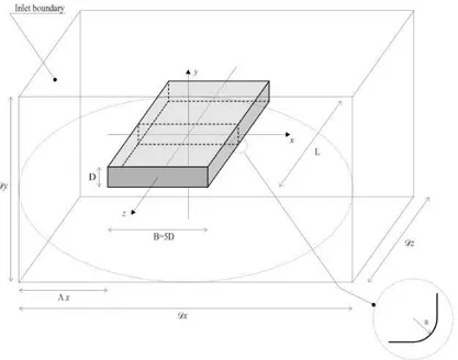
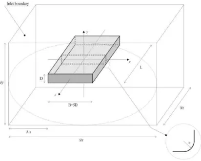
3.1 BARC computational domain . . . 17

3.2 Grid convenctions . . . 19

3.3 Grids used; 2D zoom on the horizontal plane at Z = 0 . . . 19

3.4 Flow pattern described in [3] . . . 22

3.5 Mean streamlines on the z = 0 plane. Simulations with the Smagorinsky model. . . 27

3.6 Mean streamlines on the z = 0 plane. Simulations with the WALE model. . . 28

3.7 Mean pressure coefficient at the cylinder surface s. The blue line represents the S2 case, the red one S4, the black one S2r; The cyan line represents the W2 case, the magenta one W4 and the green one W2r. The numerical data from Wei & Kareem [15] refer to a Reynold number of 10e + 4, the one from Bruno et al. [3] to Re = 4e + 4 and the ones from Mannini et al. [16] to Re = 2.64e + 4 . . . 29

3.8 Mean pressure coefficient at the cylinder surface s. Reynolds number analysis . . . 30

3.9 Mean pressure coefficient at the cylinder surface. SGS model analysis . . . 31

3.10 Mean pressure coefficient at the cylinder surface. SGS model analysis . . . 32

3.11 Absolute value of the difference between the pressure coefficient of the upper and the lower surface of the cylinder for the cases S2 and W2 . . . 33

3.12 Absolute value of the difference between the pressure coefficient of the upper and the lower surface of the cylinder for the cases S4 and W4 . . . 34

3.13 Absolute value of the difference between the pressure coefficient of the upper and the lower surface of the cylinder for the cases S2r and W2r . . . 35

(9)

4.1 Pseudo-triangular region described in [2], compared with [17] . . 37

4.2 Instantaneous streamlines snapshots on the upper surface during the vortex shedding period, on the z=0 plane (W2r simulation). Snapshots are uniformly distributed in time, and their arrange-ment is the following: from the top left to bottom left, then from top right to bottom right. . . 39

4.3 Instantaneous streamlines snapshots on the lower surface during the vortex shedding period, on the z=0 plane (W2r simulation). Same snapshots arrangement as in Figure 3.2. . . 40

4.4 Instantaneous streamlines snapshots from 816.5 to 823.25, on the z=0 plane (W2r simulation) . . . 47

4.5 Chain-like region described in [2] . . . 49

4.6 Instantaneous streamlines snapshots on the upper surface during the vortex shedding period, on the z=0 plane (S2r simulation). Same snapshots arrangement as in Figure 4.2. . . 50

4.7 Instantaneous streamlines snapshots on the lower surface during the vortex shedding period, on the z=0 plane (S2r simulation). Same snapshots arrangement as in Figure 4.2. . . 51

4.8 Instantaneous streamlines snapshots from 636 to 642.9, on the z=0 plane (S2r simulation). . . 57

5.1 Cut at z=-2, upper surface, W2r simulation . . . 60

5.2 Cut at z=-1, upper surface, W2r simulation . . . 62

5.3 Cut at z=1, upper surface, W2r simulation . . . 63

5.4 Cut at z=2, upper surface, W2r simulation . . . 64

5.5 Cut at z=-2, lower surface, W2r simulation . . . 66

5.6 Cut at z=-1, lower surface, W2r simulation . . . 67

5.7 Cut at z=1, lower surface, W2r simulation . . . 68

5.8 Cut at z=2, lower surface, W2r simulation . . . 69

5.9 Cut at z=-2, upper surface, S2r simulation . . . 73

5.10 Cut at z=-1, upper surface, S2r simulation . . . 74

5.11 Cut at z=1, upper surface, S2r simulation . . . 75

5.12 Cut at z=2, upper surface, S2r simulation . . . 76

5.13 Cut at z=-2, lower surface, S2r simulation . . . 78

5.14 Cut at z=-1, lower surface, S2r simulation . . . 79

5.15 Cut at z=1, lower surface, S2r simulation . . . 80

(10)

List of Tables

3.1 Grid characteristics . . . 18 3.2 Bulk flow parameters . . . 21 3.3 The x coordinates of the main vortex reattachment points on

both sides of the cylinder . . . 24 3.4 Bulk flow parameters . . . 26

(11)

Chapter 1

Introduction

The present work is a computational contribution to the Benchmark on the Aerodynamics of a Rectangular 5:1 Cylinder, BARC.

1.1 Benchmark description

The international Benchmark on the Aerodynamics of a Rectangular 5:1 Cylin-der has been launched in 2008 with the support of Italian and international associations ([1]). This test case is characterized by the high Reynolds number and low turbulence incoming flow around a stationary, sharp-edged rectangular cylinder of infinite spanwise length and of breadth-to-depth ratio equal to 5. In spite of the simple geometry, it is believed that the problem is of interest not only for the purpose of fundamental research, but also to provide useful infor-mation on the aerodynamics of a wide range of bluff bodies of interest in civil engineering (e.g. tall buildings, towers and bridges) and for other engineering applications.

The 5:1 aspect ratio was chosen because it is characterized by shear-layers de-taching at the upstream cylinder corners and reatde-taching on the cylinder side rather close the downstream corners. This leads to a complex dynamics and topology of the flow on the cylinder side, which adds to the vortex shedding from the rear corners and to the complex unsteady dynamics of the wake. The flow field is also known to develop three-dimensional structures.

More specifically the aims of the Benchmark are the following:

1. to deeply investigate one specific problem in the aerodynamics of bluff bodies, with contributions coming from as many researchers as possible worldwide;

2. to assess the consistency of wind tunnel measurements carried out in dif-ferent facilities;

3. to assess the consistency of computational results obtained through dif-ferent flow models and numerical approaches;

(12)

1.1 Benchmark description

4. to compare experimental and computational results;

5. to assess the possibility of developing integrated procedures relying on both experimental and computational outcomes;

6. to develop Best Practices for experiments and computations.

In addition, the results provided by the participants are meant to create a database to be made available to the scientific and technical communities for future reference. The benchmark problem was promoted by the Organizing Committee, with the support of the Italian National Association for Wind En-gineering (ANIV), under the umbrella of the International Association for Wind Engineering (IAWE) and in cooperation with the European Research Commu-nity On Flow, Turbulence And Combustion (ERCOFTAC). The following com-mon requirements are set for both wind tunnel tests and numerical simulations (see Figure 1.1):

1. Reynolds number

The depth-based Reynolds numberRe = U D/ν has to be in the range of 2 · 104 to 6 · 104.

2. Incidence

The oncoming flow has to be set parallel to the base of the rectangle; such angle of attach is termedα = 0.

3. Intensity of turbulence

The maximum intensity of the longitudinal component of turbulence is set toIu= 0.01.

4. Spanwise length of the cylinder

The minimum spanwise length of the cylinder for wind tunnel tests and three-dimensional numerical simulations is set toL/D = 3.

5. Sharpness of the section

The maximum radius of curvature of the edges of the cylinder is set to R/D = 0.05.

6. Sampling frequency

The minimum sampling frequency is set to fsD/U = 8, fs being the

(13)

1.2 Objectives

Figure 1.1: BARC computational domain

1.2 Objectives

LES is particularly attractive for the analysis of bluff body flows, which are char-acterized by a complex three-dimensional and intrinsically unsteady dynamics, that is difficult to be accurately simulated by the RANS approach. For its char-acteristics, the BARC benchmark is particularly well suited for assessment of quality and reliability of LES.

Our simulation strategy is based on the following key ingredients: (i) unstruc-tured grids, (ii) a second-order accurate numerical scheme stabilized by a nu-merical viscosity proportional to high-order space derivatives, and thus acting on a narrow band of smallest resolved scales and tuned by an ad-hoc parameter, (iii) Variational Multi-Scale (VMS) large-eddy simulation (LES) combined with eddy-viscosity subgrid-scale (SGS) model.

Focusing then on the present work, it is part of a more extended contribution to the Benchmark based on the previous ingredients, documented in [4], and the specific aims are substantially three:

1. an investigation of possible asymmetries of the mean flow on the lateral surfaces of the cylinder, and a comparison between the results using dif-ferent models;

(14)

1.2 Objectives

structures configuration;

3. a study of the three-dimensional effects of the flow features, using different models, and a comparison between the results obtained.

Considering the first two topics, they have been investigated in [3]. The present study, and the one carried out in [3] are different for many significant fea-tures, such as code of simulation, turbulence approach and modeling, flow con-ditions, and type and resolution of grid. Therefore, it is interesting to investigate whether the phenomenons described in [3] are present also in our simulations, and to eventually compare their features with those observed in [3]. Then, and this is our further contribution to BARC, we go over studying the vortical structures characteristics at different z-planes, in order to investigate the three-dimensional effects.

(15)

Chapter 2

Methodology

2.1 Large - Eddy Simulation approach

The code AERO, used in the present study, is a Navier - Stokes solver for Newtonian, compressible and three-dimensional flows. It permits to simulate laminar flows and to use different turbulence models for RANS, LES and hy-brid RANS/LES approaches.

In classical LES a spatial filter is applied to the Navier-Stokes equations in order to reduce the number of unknowns and to get rid of the small scales. Thus, only the large scales are simulated and the small scales are modeled. The spatial filter considered herein is implicitly applied by the numerical discretization. The Navier-Stokes equations for a compressible Newtonian fluid are consid-ered.The density weighted Favre filter is introduced by a ∼ and is defined as

˜

f = (¯ρf )/(¯ρ), in which the over-line denotes the grid filter. Using the Einstein summation convention they can be written as:

                   ∂ ¯ρ ∂t + ∂ ¯ρeuj ∂t = 0 ∂ ¯ρ_eui ∂t + ∂ ¯ρu_eieuj ∂xj = ∂ ¯ρ ∂xi +∂(µσfij) ∂xj −∂M (1) ij ∂xj +∂M (2) ij ∂xj ∂(¯ρ eE) ∂t + ∂[(¯ρE + ¯p)euj] ∂xj = −∂(eujσfij) ∂xi − ∂qej ∂xj +∂(Q (1) j +Q (2) j +Q (3) j ) ∂xj (2.1)

where µ is the viscosity, p is the pressure, E is the total energy, ui is the

velocity component in the i direction,q_ej is the resolved heat flux. The tensor

f σij is defined as: f σij = − 2 3Sgkkδij+ 2 fSij (2.2)

(16)

2.1 Large - Eddy Simulation approach

f

Sij being the resolved strain tensor:

f Sij = 1 2( ∂_eui ∂xj +∂uej ∂xi ) (2.3)

In modeling the SGS terms resulting from filtering the Navier-Stokes equations, it is assumed that low compressibility effects are present in the SGS fluctuations. We also assume that the heat transfer and temperature gradients are moderate. The SGS term in the momentum equation is thus given by the classical stress tensor:

M_ij(1)=ρuiuj− ρueiuej (2.4)

and by the SGS term M_ij(2) that takes into account the transport of viscous term due to the small scales fluctuations. Mij(2)can be neglected because we are

interested in high Reynolds number flows.

The isotropic part of Mij can also be neglected under the assumption of low

compressibility effects in the SGS fluctuations, [4]. The deviatoric part,Tij can

be expressed by an eddy-viscosity term as follows:

Tij= −2µsgs( fSij−

1

3Sgkk) (2.5) where µsgs the SGS viscosity. In the total energy equation, the effect of the

SGS fluctuations are modeled by introducing a constant SGS Prandtl number to be fixed a priori:

P rsgs=Cp

µsgs

Ksgs

(2.6)

where Ksgs is the SGS conductivity coefficient. It takes into account the

dif-fusion of total energy due to SGS fluctuations. In the filtered and normalized equation of energy, this term is added to the molecular conductivity coefficient. Two different eddy-viscosity SGS models are used in the present work. The first one is the classical Smagorinsky model extended to a compressible flow ([5]), and the second is the Wall-Adapting Local Eddy -Viscosity model (WALE), ([6]).

(17)

2.2 Smagorinsky Model

The SGS eddy-viscosity Smagorinsky model is the best known closure model. It is well known that this model has some drawbacks but thanks to the simplicity of implementation and the low computational costs it is very attractive for complex industrial applications. For the classical Smagorinsky model the eddy-viscosity µsgs is defined as follows: µsgs=ρ(Cs∆)2 Se , (2.7) Se = q 2 fSijSfij (2.8)

where ∆ is the filter width andCs is a specific constant that must be a priori

assigned. The value typically used for shear flows ofCs= 0.1 is adopted herein.

The grid width filter corresponding to the numerical discretization must be computed. The filter for each grid element is defined herein as follows:

∆(l)=V ol(Tl) 1

3 (2.9)

in whichV ol(Tl) is the volume of thelthtetrahedron of the mesh.

Many studies have shown that the value assigned to the constantCs plays an

important role in the quality of the simulation. Moreover the Smagorinsky model suffers of the follow drawbacks:

1. a wrong behaviour of the flow is predicted in the near wall region,Tij not

vanishing with the correct trend;

2. only a dissipative effect of the small scales is obtained and so it becomes impossible to properly take into account the backscatter of energy from the small scales to large scales;

3. it is not able to properly handle transition, since the SGS viscosity does not vanish for laminar flows with shear.

This was partially overcame with the appearance of the dynamic version of the Smagorinsky model, [5]

In this method, the constantCsis calculated during the simulation and takes a

local value, obtained from the smallest resolved scales, which can be negative. This local value is calculated using an algebric equation and using a coarser filter than the one applied to the Navier-Stokes equations.

The Germano model overcomes all the above mentioned problems of the Smagorin-sky model. However, if too high fluctuations in the value ofCsappear during a

simulation, this can lead to instabilities. On unstructured meshes, the increase in complexity is rather large and also the computational costs. In contrast, the

(18)

2.3 WALE model

variational multi-scale (VMS) approach, described in the following, might be effective in obtaining a good compromise between accuracy and computational requirements. To improve the behaviour in the near wall region, another solu-tion is to use other expressions for the turbulent viscosity term. The WALE model is an examples of closure model of this type.

2.3 WALE model

WALE (Wall-Adapting Local Eddy -Viscosity) is a subgrid scale model which was introduced by [6].

This model is based on the square of the velocity gradient tensor. It detects the effects of the smallest resolved turbulent fluctuations relevant for the kinetic energy dissipation. Moreover it has the the correct behaviour near the walls without using a dynamic procedure neither a damping function. The model produces zero eddy viscosity in the case of pure share being therefore able to handle the laminar to turbulent transition.

The eddy-viscosity termµwaleis defined as:

µwale= (Cw∆)2 (Sd ijSijd) 3 2 (SijSij) 5 2 + (Sd ijSijd) 5 4 (2.10)

whereCwis a constant and is fixed to 0.5,as proposed in [6],

Sijd = 1 2(g 2 ij+gji2) − 1 3δijg 2 kk (2.11) and, g2ij=gikgkj. (2.12)

(19)

2.4 Numerical method

The numerical code considered herein (AERO) employs unstructured, tetrahe-dral grids. A mixed finite-volume/finite-element method is used for the space discretization. The finite-volume formulation is used for the convective terms and finite-elements (P1-Galerkin) for the diffusive terms. The spatial discretiza-tion scheme is vertex centered, i.e. all degrees of freedom are located at the vertices.

The computational domain is approximated by a polygonal domain. A dual finite-volume grid is obtained by building a cellCi around each vertex i. The

finite-volume cells are built by the rule of medians: the boundaries between cells are made of triangular interface facets. Each of these facets has a mid-edge, a facet centroid, and a tetrahedron centroid as vertices. The convective fluxes are discretized on this tessellation by a finite-volume approach. The Roe scheme (with low-Mach preconditioning) represents the basic upwind component for the numerical evaluation of the convective fluxes F :

R ∂Ci F (W, ~n)dσ ' ΦR_(W i, Wj, ~n) = F (Wi, ~n) + F (Wj, ~n) 2 | {z } centered − γsdT(Wi, Wj, ~n) | {z } upwinding (2.13) dR_(W i, Wj, ~n) = P−1|P R(Wi, Wj, ~n)| Wj− Wi 2 (2.14) in whichWi is the solution vector at theith node, ~n is the normal to the cell

boundary andR is the Roe Matrix.

The matrixP (Wi, Wj) is the Turkeltype preconditioning term, introduced to

avoid accuracy problems at low Mach numbers ([7]). Note that, since it only appears in the upwind part of the numerical fluxes, the scheme remains consis-tent in time and can thus be used for unsteady flow simulations.

The parameterγs has been introduced, which directly controls the spatial

dis-sipation of the scheme. It leads to a full upwind scheme (the usual Roe scheme) whenγs= 1 and to a centered scheme whenγs= 0.

The spatial accuracy of this scheme is only first order. The MUSCL linear re-construction method (Monotone Upwind Schemes for Conservation Laws), in-troduced by Van Leer, is therefore employed to increase the order of accuracy of the Roe scheme. It is compatible with vertex-centered and edge-based formula-tions, allowing rather easy and inexpensive higher-order extensions of monotone upwind schemes on Cartesian grids. The basic idea consists in expressing the Roe flux as a function of a reconstructed value of W at the boundary between the two cells centered respectively at nodes i and j. A reconstruction using a combination of different families of approximate gradients is adopted ([8]). This allows a numerical dissipation made of sixth-order space derivatives to be obtained.

(20)

2.5 Variational MultiScale LES approach

An implicit time advancing algorithm is used, based on a second-order time-accurate backward difference scheme, which involves an explicit time derivative expressed only as a spatial residual, so that it does not depend on time step length. A first-order semi-discretization of the jacobians is adopted together with a defect correction procedure ([9], [10]). The resulting method is second order accurate in space and time and allows stable calculations to be carried out on very heterogeneous grids (with locally very small cells) and for a large range of Mach numbers. For a more detailed description of the AERO code, we refer to [8] and [11].

2.5 Variational MultiScale LES approach

The variational multiscale (VMS)approach, introduced in [12], might be ef-fective in obtaining a good compromise between accuracy and computational requirements. In this approach, the scales resolved on the computational grid are further split into the largest resolved scales (LRS) and the smallest resolved scales (SRS). This is done through a classical Galerkin projection onto a coarser grid made of macro-cells. The macro-cells are obtained by a process known as agglomeration [13] (see Figure 2.1). The key point in VMS LES is that SGS

Figure 2.1: Cell agglomeration method

model (in our case either the Smagorinsky or the WALE model) is applied only to the SRS. This allows the excessive dissipation introduced by eddy-viscosity SGS models also on the large scales to be reduced.

(21)

Chapter 3

Test-case description and

validation

3.1 Test-case and simulation setup

Simulations are carried out for the flow around a fixed sharp-edged rectangular cylinder with a chord-to-depth ratio, B/D, equal to 5. The angle of attack is zero and two different values of the Reynolds number are considered, namely ReD = U∞D/ν = 20000 and 400000, U∞ being the free-steam velocity, D

the cylinder depth andν the fluid kinematic viscosity. The free-stream Mach number is set equal to M∞=0.1 in order to make a sensible comparison with

incompressible simulations. Preconditioning is used to deal with the low Mach number regime.

The computational domain is: −15.5 ≤ x/B ≤ 25.5, −15.1 ≤ y/B ≤ 15.1, −0.5 ≤ z/B ≤ 0.5, where x, y and z denote the streamwise, transverse and span-wise directions respectively, the cylinder center being located atx = y = z = 0 (see Figure 3.1).

In the spanwise direction, periodic boundary conditions are imposed, while characteristic-based conditions are used at the inflow and outflow as well as on the lateral boundaries (y/B = ±15.1). A slip condition is imposed on the velocity at a distanceδ from the wall. In our case we consider δ = 0.002D. The Reichart wall-law (see equation 2.3) is used to derive the shear stresses caused by the presence of the wall. This law has the advantage of describing the velocity profile not only in the logarithmic region of a turbulent boundary layer, 40 ≤y+_{, but also in the laminar sublayer,} _y+ _{≤ 3, and in the}

interme-diate region. This also guarantees correct asymptotic behaviour at the wall of the SGS terms in the Smagorinsky model.

y+_{is defined as a non-dimensional parameter:}

y+₌ρuf

(22)

3.1 Test-case and simulation setup

Figure 3.1: BARC computational domain

where, for our cases,y = δ. The velocity uf is also called friction velocity:

uf =

r_τ

ω

ρ (3.2)

whereτω is the shear stress tension at the wall.

The Reichart wall-law has the following expression [equation 2.3]:

u+₌ 1 kln(1 +ky +_{) + 7.8(1 − e}y+₁₁ ₋y + 11e − 0.33y +₎ _(3.3)

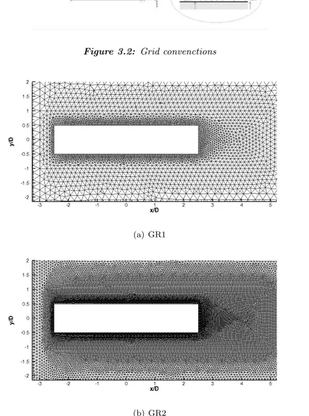
Two different grids have been used, both are unstructured and made of tetra-hedrons with approximately 2.09 · 105 _{cells for the coarse one (GR1), see}

Fig-ure 3.3(a), and 9.5 · 105 _{cells for the finer one (GR2), see Figure 3.3(b). The}

minimum grid resolution in the spanwise direction, i.e. those of the nodes on the cylinder surface, is constant: ∆zmin/D = 0.2085 for GR1, and ∆zmin/D = 0.05

fro GR2, see also Table 3.1. The grid resolution grows and becomes non-homogeneous moving away from the cylinder, so that the maximum values are: ∆zmax/D = 1 for GR1, and ∆zmax/D = 2.5 for GR2.

(23)

be-3.1 Test-case and simulation setup

Grid ∆xmin ∆ymin ∆zmin

GR1 0.05 0.0412 0.2085 GR2 0.025 0.0213 0.05

Table 3.1: Grid characteristics

wall, see Figure 3.2. For GR1 its maximum value ismax(nw) = 0.0489D, its minimummin(nw) = 0.0412D and its averaged value is avg(nw) = 0.0441D. For GR2 thenw values are: max(nw) = 0.0236D, min(nw) = 0.0213D, and avg(nw) = 0.023D. It is estimated a posteriori that the first node is located approximately aty+_{∈ [1, 20] in GR1, and y}+_{∈ [0.9, 14] in GR2.}

For more details concerning the grids, see [4]

As for modeling, the Smagorinsky and WALE models were used for the VMS-LES approach and the free parameter in the WALE SGS model is set equal to Cw = 0.5, as suggested in [6] and the one in the Smagorinsky model equal to

Cs= 0.1. The filter width is defined as the third root of the volume of the grid

elements, and the macro-cells used in the VMS procedure are obtained from the finite-volume cells associated to the computational grid by means of one level of agglomeration (see Section 1.5).

(24)

3.1 Test-case and simulation setup

Figure 3.2: Grid convenctions

(a) GR1

(b) GR2

(25)

3.2 Validation

The present work is a part of a research activity aimed at investigating the sensitivity to the SGS model, grid resolution and Reynolds number. Therefore, for each of the SGS models three different simulations were carried out: ReD=

20000 on GR1 (S2 and W2) and on GR2 (S2r and W2r) andReD= 40000 on

GR1 (S4 and W4).

More specifically, the simulations S2r, W2, W4, and W2r were carried out within the present thesis.

As for numerics, the parameter controlling the amount of numerical viscosity, γsis set to 0.3 for the simulations S2 and S4, while it is increased to 0.5 for the

other four simulation. This increment of the value ofγsis due to some

numeri-cal stability problems. Nonetheless, it has been observed in our previous studies that for this range of values the impact of numerical viscosity on the results may be considered negligible. In all cases, the governing equations were advanced in time starting from initial conditions in which the velocity is assumed to be uniform and equal to the free-stream velocity. The adopted time step is fixed such that the CFL number is equal to 20. A preliminary sensitivity analysis was carried out by varying the CFL number from 10 to 30 and no significant differences were observed in the results.

The simulations have been performed thanks to the Cineca PC cluster (IBM Power6, 4.7 GHz,21 TB (128 GB/node)) and to the Caspur PC cluster (IBM SP, 2-way quad-core Opteron 2.1GHz with 16 GB of RAM/node). The simulations for the coarse grid were performed using eight processors and the simulations on GR2 using 48 processors. The simulations W2, W4 and W2r were carried out on the Caspur cluster, using for W2 a total of 100h × 8 and for the simulation W2r 100h × 48.

3.2 Validation

The aerodynamic force coefficients are defined as follows:

Cl= ₁ l 2ρU 2_S Cd= d 1 2ρU 2_S

wherel is the global lift and d is the global drag, ρ and U are the free-stream flow density and velocity andS is the reference surface. U∞ is also considered

the reference velocity andS in our case is equal to D, the reference length. For the validation, the convergence of the mean values and root mean square of the drag and lift coefficients have been checked for increasing extents of the time interval, ∆tn, used to compute the statistics. The results are reported

and explained in [4], and these values are in good agreement with the available experimental data and also with the numerical results. The main flow bulk parameters obtained in the simulations studied in [4] and in the present work

(26)

3.2 Validation

are shown in Table 3.2, however a detained comparison of this bulk parameters with available numerical and experimental data is carried out in [4]. Our results are in general good agreement with literature data.

In particular we remark herein that the time fluctuations of lift std(Cl) are

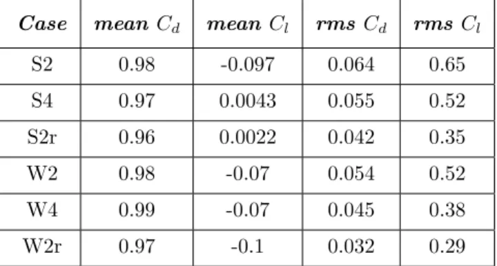
Case mean Cd mean Cl rms Cd rms Cl

S2 0.98 -0.097 0.064 0.65 S4 0.97 0.0043 0.055 0.52 S2r 0.96 0.0022 0.042 0.35 W2 0.98 -0.07 0.054 0.52 W4 0.99 -0.07 0.045 0.38 W2r 0.97 -0.1 0.032 0.29

Table 3.2: Bulk flow parameters

very sensitive even to small modification of the flow dynamics and, more specif-ically, to the characteristics of the flow on the cylinder side surface. A large spreading is observed also in the literature for this quantity. Compared with the only available experimental data all the numerical results are rather large. The impact of the SGS model on this quantity is large(S2 vs. W2, S2r vs. W2r) and the grid effects are also very strong (S2 vs. S2r, W2 vs. W2r). Considering these observations, modifications are expected in the flow topology and in the pressure distribution on the cylinder for the different simulations (see Section 1.2.1 and 1.2.2). It can be also observed that the Reynold number effects are not negligible (S2 vs. S4, W2 vs. W4).

Finally, for our simulations themean(Cl) is always rather low, as expected,

ex-cept for the simulation W2r. Because a check of the convergence of the averaged quantities is made it may be assumed that a value significantly different from zero is an indication of an asymmetry of the mean flow. Indeed, for the W2r simulation, the mean flow has been found to be noticeably asymmetric. Wei & Kareem [15] and Bruno et al. [3] found rather high values formean(Cl).

This may be due to a small time interval used to compute the average quanti-ties. Nonetheless, in Bruno et al. [3] a check of the convergence of the averaged quantities is made, and, hence,in this case, the statistical sample may be as-sumed to be adequate. Therefore, it can be argued that, like in our case, this high value is determined by a large asymmetry in the mean flow. This issue will be investigated more.

(27)

3.2 Validation

3.2.1 Mean flow topology

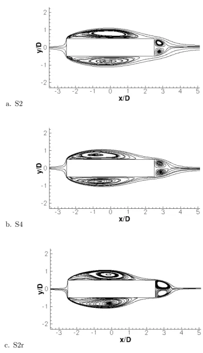
The topology of the mean flow around the cylinder is shown in Figure 3.5 and Figure 3.6, where the streamlines obtained from the velocity field averaged in time are plotted on the plane at z = 0.

We will analyse the mean flow topology obtained in the present simulations

Figure 3.4: Flow pattern described in [3]

on the plane at z = 0 (for more details see [4]). For both the simulations car-ried out on the refined grid we find a mean flow pattern very similar to that in Figure 3.4 taken from a large eddy-simulation of the same flow configuration [3]. In this figure the streamlines of the solution averaged in time and along the spanwise direction are plotted in the upper part of the figure while a syn-thetic sketch of the recognized mean flow structures is plotted in the lower part. The mean flow separates at the leading edge and reattaches just upstream the trailing edge. The main vortex shows an inclined major axis. In our cases this axis is just slightly inclined, less than in Figure 3.4. In this Figure, Bruno et al. [3] individuates a thin recirculation region, clearly visible close to the lateral wall, between the main vortex and the separation point. In a large flow region between the main vortex and the recirculation region, called inner “region “, no mean structures can be easily recognized.

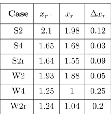
Considering our simulations, in all cases, a large recirculation region on the cylinder side and one in the wake immediately behind the cylinder are clearly visible. However, their characteristics are not the same for the different simu-lations. In order to assess the differences, we evaluated the length of the mean recirculation zone on the cylinder sides, xr, see Table 3.3. xr represents thex

coordinate of the reattachment point, which has been estimated from the mean velocity field;x+

r andx−r are the coordinates of the reattachment point on the

upper and lower sides of the cylinder. An asymmetry between the length of the lower recirculation zone and length of the upper one can be observed in Table 3.3. Therefore we computed and reported in Table 3.3 ∆xr= |x+− x−|.

The most asymmetric case is found to be W4, followed by W2r. The issue of the asymmetry of the mean flow will be discussed in more details in the following (see Section 3.2.2).

(28)

Ta-3.2 Validation

ble 3.2, and 3.3 the following conclusions on the effects of the different considered parameters can be drawn:

1. Increasing the Reynolds number the length of the main vortexes decreases considerably, the core of the vertex moves upstream and the normal dis-tance of the core to the surface slightly decreases (see S2 vs S4 and W2 vs W4). For instance, the reattachment point on the cylinder side is located approximately atxr = 2D for the simulation S2, while it moves upstream

as the Reynolds number increases (xr' 1.7D for S4).

2. Refining the grid a secondary recirculation zone downstream the leading corner is observed, the center of the primary vortex moves slightly down-stream and at a larger normal distance from the side surface, see Table 3.2, and 3.3. The reattachment point moves upstream and the curvature of the mean streamlines is larger (S2 vs S2r and W2 vs W2r).

3. The previous trends are observed for both SGS models even though the quantitative results are different.

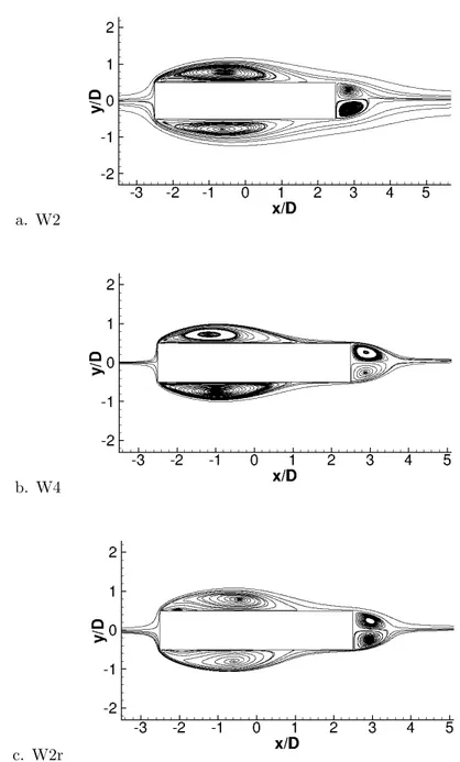
4. The SGS model has a strong effect on the prediction of the reattachment point; indeed, in the simulations with the WALE model it is always up-stream that the one in the corresponding simulation with the Smagorinsky model. Indeed, in the simulations with the WALE model the main vor-texes are shorter and their core is placed upstream than the main vorvor-texes in the the corresponding simulations with the Smagorinsky model.

Summarizing, the length and shape of the mean streamlines are different for the different simulations and this may explain the different behaviour of the mean pressure coefficient which will be analysed in the following section.

(29)

3.2 Validation Case xr+ x_r− ∆x_r S2 2.1 1.98 0.12 S4 1.65 1.68 0.03 S2r 1.64 1.55 0.09 W2 1.93 1.88 0.05 W4 1.25 1 0.25 W2r 1.24 1.04 0.2

Table 3.3: The x coordinates of the main vortex reattachment points on both sides of the cylinder

3.2.2 Pressure distribution over the cylinder surface

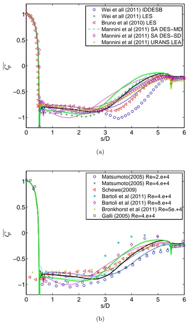
The mean pressure coefficient is plotted in Figure 3.7 as a function of the co-ordinate s for the upper side of the cylinder (defined in Figure 3.2) and com-pared with the numerical (Figure 3.7(a)) and experimental data in literature (Figure 3.7(b)). Small wiggles are observed in the present simulations at the cylinder corners. This is due to numerical problems connected with a too coarse grid resolution and indeed, the wiggles are reduced on GR2. They could be eliminated by carrying out a further local refinement. All the present results are well inside the experimental range and in good agreement with the values of other numerical contributions to the benchmark. It seems that the numerical results are less scattered that the experimental results, even though different numerical approaches were used (see [4] for more details).

Let us now analyse in more details the effects of the different parameters on our results. The influence of the Reynolds number on the mean pressure distribution can be observed in Figure 3.8 where the comparison S2 vs S4 and W2 vs W4 are displayed. Increasing the Reynolds number the minimum value ofCp decreases as well as the length of the plateau, being in good agreement

with the decreasing length of the main recirculation zone. For all the cases the length of the pressure coefficient plateau corresponds to the length from the leading corner to the center of the main vortex.

It can be remarked that, for both considered SGS models, the trend with the Reynolds number remains the same.

The SGS model (Figure 3.9) and the grid refinement (Figure 3.10) have also an impact on the mean pressure coefficient distribution results. It can be seen that the base pressure is practically the same for all the cases, consistently with the fact that the mean drag coefficient is almost the same for all the present simulations.

Let us analse now the effects of grid refinement. The topology of the flow for the simulations carried out on the refined grid changes and a secondary

(30)

3.2 Validation

a. S2

b. S4

c. S2r

Figure 3.5: Mean streamlines on the z = 0 plane. Simulations with the Smagorinsky model.

(31)

3.2 Validation

a. W2

b. W4

c. W2r

Figure 3.6: Mean streamlines on the z = 0 plane. Simulations with the WALE model.

(32)

3.2 Validation 0 1 2 3 4 5 6 −1 −0.5 0 0.5 1 s/D Cp

Wei et all (2011) IDDESB Wei et all (2011) LES Bruno et al (2010) LES

Mannini et al (2011) SA DES−MD Mannini et al (2011) SA DES−SD Mannini et al (2011) URANS LEA

(a) 0 1 2 3 4 5 6 −1 −0.5 0 0.5 1 s/D Cp Matsumoto(2005) Re=2.e+4 Matsumoto(2005) Re=4.e+4 Schewe(2009) Bartoli et al (2011) Re=4.e+4 Bartoli et al (2011) Re=8.e+4 Bronkhorst et al (2011) Re=5e.+4 Galli (2005) Re=4.e+4 (b)

Figure 3.7: Mean pressure coefficient at the cylinder surface s.

The blue line represents the S2 case, the red one S4, the black one S2r; The cyan line represents the W2 case, the magenta one W4 and the green one W2r. The numerical data from Wei & Kareem [15] refer to a Reynold number of 10e + 4, the one from Bruno et al. [3] to Re = 4e + 4 and the ones from Mannini et al. [16] to Re = 2.64e + 4

(33)

3.2 Validation

recirculation zone appears at the upstream corners, Figure 3.10. The length of theCp plateau downstream the separation point is shorter for the simulations

on GR2 with respect to the ones on GR1.

TheCpdistributions on the lateral cylinder side is characterized by a plateau

in the upstream zone, where almost constant low pressure can be observed and, in the downstream zone, by a zone where the pressure starts to increase. This evolution is in correlation with the mean flow topology, shown in the previous Section. A short recirculation zone determines a larger normal distance from the side surface to the centre of the vortex, higher curvature of the mean streamlines, that in terms ofCp can be translated in a rapid increase ofCp with an abrupt

slope.

3.2.3 Analysis of asymmetries in the mean flow

We investigate now in more detail the asymmetry of the mean flow on the two different cylinder lateral surfaces, suggested by the non-zero values of the mean lift (see Table 3.2, and the previous relevant discussions).

The WALE cases are the ones with larger asymmetry. We are sure that the asymmetry is not due to a too short time interval considered for computing the averaged results of the simulation since we checked the convergence of statistical quantities.

In order to do a more quantitative assessment of the asymmetries we define and analyse:

∆Cpmax =max(|Cpupper(x) − Cplower(x)|) (3.4)

∆Cpavg =avg(|Cpupper(x) − Cplower(x)|) (3.5)

∆Cp(%) =max

|Cpupper(x) − Cplower(x)|

(Cpupper(x) − Cplower(x))/2

(34)

3.2 Validation

Case ∆Cpavg ∆Cpmax ∆Cp(%)

S2 0.027 0.062 3.7 S4 0.012 0.05 3.83 S2r 0.0077 0.063 1.3 W2 0.017 0.037 5.72 W4 0.035 0.089 2.22 W2r 0.021 0.066 2.83

Table 3.4: Bulk flow parameters

The results are presented in Table 3.4. The points at the corners are excluded for the simulations carried out on the coarse grid, because of the presence of numerical wiggles, as previously discussed.

Examining the values obtained in Table 3.4 we notice that indeed the simulation W4 has the largest peak of asymmetry but it is not the most asymmetric case, this being W2. It can be remarked that by refining the grid the asymmetry decreases.

All of the results presented above are referred to the solution averaged in time on the plane z = 0. In order to confirm the observation made in this section the absolute value of the difference between the pressure coefficient of the upper and lower surface along the whole spanwise domain length of the cylinder was plotted and investigated. The results are presented in Figure 3.11, 3.12 and 3.13.

In all the figures it is easy to observe that the leading and trailing corners zones present the wiggles individuated also in theCp graphs (Figure 3.7). As noticed

before, by refining the grid the difference in the Cp values in these zones are

not so high anymore and it can be seen that the zone where the wiggles can be observed is less extended. Also the asymmetry zones become more compact and better defined.

The case W4 is the most asymmetric, having peaks of asymmetry of 10% and a large zone with 8% of asymmetry (see Figure 3.12). The case S2r is the most symmetric one. For the simulations with the Smagorinsky SGS model on GR1 the solution is more asymmetric for the smaller Reynolds number, the opposite can be said about the simulations carried out with the WALE SGS model. In all cases it seems that the zone where the asymmetry is always present is the one contained between the center of the vortex and the end of the main separation zone. This finding is not in agreement with the results in [3], in which the most asymmetric zones are located between the leading corners of the cylinder and the vortex core.

(35)

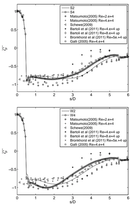
3.2 Validation 0 1 2 3 4 5 6 −1 −0.5 0 0.5 1 s/D Cp S2 S4 Matsumoto(2005) Re=2.e+4 Matsumoto(2005) Re=4.e+4 Schewe(2009) Bartoli et al (2011) Re=4.e+4 up Bartoli et al (2011) Re=8.e+4 up Bronkhorst et al (2011) Re=5e.+4 up Galli (2005) Re=4.e+4 0 1 2 3 4 5 6 −1 −0.5 0 0.5 1 s/D Cp W2 W4 Matsumoto(2005) Re=2.e+4 Matsumoto(2005) Re=4.e+4 Schewe(2009) Bartoli et al (2011) Re=4.e+4 up Bartoli et al (2011) Re=8.e+4 up Bronkhorst et al (2011) Re=5e.+4 up Galli (2005) Re=4.e+4

Figure 3.8: Mean pressure coefficient at the cylinder surface s. Reynolds number analysis

(36)

3.2 Validation 0 1 2 3 4 5 6 −1 −0.5 0 0.5 1 s/D Cp S2 W2 Matsumoto(2005) Re=2.e+4 Matsumoto(2005) Re=4.e+4 Schewe(2009) Bartoli et al (2011) Re=4.e+4 up Bartoli et al (2011) Re=8.e+4 up Bronkhorst et al (2011) Re=5e.+4 up Galli (2005) Re=4.e+4 0 1 2 3 4 5 6 −1 −0.5 0 0.5 1 s/D Cp S4 W4 Matsumoto(2005) Re=2.e+4 Matsumoto(2005) Re=4.e+4 Schewe(2009) Bartoli et al (2011) Re=4.e+4 up Bartoli et al (2011) Re=8.e+4 up Bronkhorst et al (2011) Re=5e.+4 up Galli (2005) Re=4.e+4

Figure 3.9: Mean pressure coefficient at the cylinder surface. SGS model anal-ysis

(37)

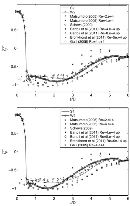
3.2 Validation 0 1 2 3 4 5 6 −1 −0.5 0 0.5 1 s/D Cp S2r W2r Matsumoto(2005) Re=2.e+4 Matsumoto(2005) Re=4.e+4 Schewe(2009) Bartoli et al (2011) Re=4.e+4 up Bartoli et al (2011) Re=8.e+4 up Bronkhorst et al (2011) Re=5e.+4 up Galli (2005) Re=4.e+4

Figure 3.10: Mean pressure coefficient at the cylinder surface. SGS model anal-ysis

(38)

(39)

3.2 Validation

(40)

(41)

Chapter 4

Analysis on the z=0 plane

4.1 Analysis for the W2r simulation

At this point of our investigation an analysis of the flow configuration on the symmetry plane,z = 0, is made for both models of simulation. We consider the simulations carried out atRe = 20000, on the more refined grid, with both SGS models.

In particular, in each case a vortex shedding period is considered, in order to describe the flow features in a short and significant period of time.

Furthermore this analysis is made for both the upper and the lower surface of the cylinder, since different types of vortex structures at different times can be recognized, and a possible interaction between them is studied. The WALE model is first considered.

4.1.1 Upper surface

For the upper surface of the cylinder an adimensional vortex shedding period tU/D is considered, where t is the time in seconds, U the free-stream velocity and D the cylinder depth. The adimensional time interval is 817.5 − 820.55, and it is divided into 12 time-steps, each one of 0.225. In this way the flow can be analysed almost instantaneously while the vortex shedding occurs.

Considering Figure ??, the instantaneous streamlines are visualized, not for all the cylinder depth, but just for a fraction, in particular the same one used in [2], in order to make an accurate comparison with that work. It is possible to immediately recognize the pseudo-triangular zone identified in [2]: V1 and V2 are the elongated clockwise ”bubbles” in the shear layer, just downstream the leading edge, and there is V3, which is the counter-clockwise vortex close to the cylinder upper surface, which is streaming to the leading edge because of the velocity field induced by the other two vortices. V4 is the vortex that has just shed and is moving downstream, where it is going to interact with the other structures.

(42)

4.1 Analysis for the W2r simulation

be noticed that V3, during the latest time-steps is including other smaller clock-wise vortices, creating just one, more intense, vortex.

Then the phenomenon described in [2] is perfectly recognized: it reminds of what explained by Pullin & Perry in 1980 in [17]; in fact, looking at Figure 4.1 the same nomenclature is adopted.

It is very important to highlight that the present work and the one in [2] are very different for many important features, such as flow conditions (from Reynolds number to the code for simulation) and type of grid used, but the results are similar. This implies that the pseudo-triangular region is effectively a pecu-liar phenomenon of the flow around this body, even if the flow conditions are different.

Figure 4.1: Pseudo-triangular region described in [2], compared with [17]

4.1.2 Lower surface

For the lower surface we decided to investigate not the same vortex shedding period as for the upper surface: in this case the adimensional time interval is 816.5 − 819.2, so it is in practice the previous vortex shedding period with re-spect to the one considered for the upper surface. The number of instantaneous streamlines snapshots, and the length of the time-step, are the same in both cases.

Concerning this case, and considering Figure 4.3, we can find three vortices at the leading edge: it is a sort of pseudo-triangular region. In fact, there are V1 and V3, the two counter-clockwise vortices, and there is also V2, the clockwise vortex near to the body surface. It is possible to observe that V1 seems to be the elongated bubble from which the vortex is shed, and looking at the second column of Figure 4.3, we can notice that V3 is not visible anymore: in fact, it is not as V1, but it is just a structure involved in the shedding. Obviously V3

(43)

counter-clockwise vortex downstream.

This phenomenon is not exactly as that described in [2], but it is very similar, since the vortex shedding mechanism from the elongated bubble is present, and the number of main structures is three, two rotating likewise and another one nearest to the body counter-rotating, like in the pseudo-triangular region. So the region identified and described in [2] is present in both surfaces.

In order to make a more complete and accurate investigation of the interaction between the structures on the upper and lower surface, the flow around the whole cylinder lateral surface is analysed in the next Section.

(44)

Figure 4.2: Instantaneous streamlines snapshots on the upper surface during the vortex shedding period, on the z=0 plane (W2r simulation).

Snapshots are uniformly distributed in time, and their arrangement is the follow-ing: from the top left to bottom left, then from top right to bottom right.

(45)

v

₁

v

1

v

₂

v

₂

v

₃

1.75 D

Figure 4.3: Instantaneous streamlines snapshots on the lower surface during the vortex shedding period, on the z=0 plane (W2r simulation).

(46)

4.1.3 Flow around the cylinder

As stated above, two different vortex shedding periods have been considered for the upper and lower surfaces, in particular the first one almost comes after the second one. This is not a random choice, but to better explain our observations about the flow features and the possible interaction of the vortex structures between the two cylinder surfaces. We analyse herein the flow dynamics over the entire cylinder surface.

Looking at Figure 4.4, the instantaneous vorticity fields for more than a vortex shedding period are visualized: in particular there are 30 instantaneous fields, for the time interval 816.5 − 823.25.

An investigation about a possible interaction between the structures on upper and lower cylinder surfaces has been made, and a sort of alternation of the pseudo-triangular region on the two surfaces has been noticed.

Considering Figure 4.4, the sub-figures from 1 to 12 are the ones analysed in 4.1.1, so the triangular region is identified on the lower surface, but looking at the upper one, the region is absolutely not recognizable. In fact, there is just a sort of elongated bubble at the leading edge, but the other two structures, peculiar for the triangular region, are not present.

Let us consider the following vortex shedding period, sub-figures from 13 to 25, which is almost the one considered in 4.1.2. From sub-figure 16 it is clearly pos-sible to notice that the pseudo-triangular region is present on the upper surface, but on the lower one, it is impossible to identify the same trend, or better, it is not possible to identify any trend.

We have just considered the particular vortex shedding period studied previ-ously, but let us go through the rest of instantaneous fields visualized. From sub-figure 25 to the end it is possible to observe that the triangular region re-mains on the upper surface, but we cannot find the same on the lower surface yet. This could lead us to the idea of an unsymmetrical alternation of the tri-angular region between up and down the cylinder, since we can certainly affirm that when it is on a surface, it is not on the other one, but the time length dur-ing which it remains on one is not the same for the two surfaces, but it seems to be larger on the upper surface.

It cannot be excluded that this may depend on the particular vortex shedding period chosen, so at this point it is not possible to be certain that this is a general behaviour of the flow around this particular body. This is the reason why a simulation with another model has been analysed, and not just for the symmetry plane, so that examining the instantaneous streamlines snapshots on different planes, we can try to define a more general trend.

The same analysis with the Smagorinsky model and a comparison between the results in Section 4.2 will be made.

(47)

4.1 Analysis for the W2r simulation 1. 2. 3. 4. 5.

(48)

(49)

(50)

(51)

(52)

Figure 4.4: Instantaneous streamlines snapshots from 816.5 to 823.25, on the z=0 plane (W2r simulation)

(53)

4.2 Analysis for the S2r simulation

In this section the flow on the symmetry plane is analysed for the simulation using the Smagorinsky model. The flow conditions and the grid used are the same as W2r.

4.2.1 Upper surface

Let us consider the cylinder upper surface, in this adimensional vortex shedding period: 641.06 − 643.82, with time-step 0.23, which is slightly shorter than the W2r case. The number of instantaneous streamlines snapshots, and the cylinder depth visualized are the same in all cases.

Looking at Figure 4.6 the pseudo-triangular region is immediately

recognizable: V1 is the elongated clockwise bubble from which the vortex V2 has just shed, and V3 is the counter-clockwise vortex near to the surface. In this case the dynamics of the vortex shedding is very well represented, since the main structures are easy to be detected, and the position of the vortices along the time-steps is tracked very satisfactorily.

Indeed, the upstream movement of the V3 vortex, because of the flow induced by V1 and V2, which are much more intense and counter-rotating, is very clear and long.

So, the triangular region is still present, even if the SGS model is different. Let us then analyse the lower surface.

4.2.2 Lower surface

For the lower surface the analysed adimensional vortex shedding period is almost the former of the one considered in 4.2.1, and in particular it is 636.23 − 638.99. The number of instantaneous streamlines snapshots is the same as above. Con-sidering Figure 4.7 the cylinder lower surface presents a completely different flow configuration from the other described above. In this case we have more structures, in particular there are five main vortices, three shed from the leading edge which are counter-clockwise, and the other two clockwise near to the body surface. This trend is also detected in [2], and reported in Figure 4.5: it is differ-ent from the pseudo-triangular region, because of the longer number of vortices present. In the following this trend is going to be called chain-like region, which is different from the pseudo-triangular one because there are more than two structures shed from the leading edge, and more than one counter-rotating near to the cylinder.

The chain-like is going to be defined as the region where there are at least three likewise rotating vortices shed from the leading edge and moving downstream, and two counter-rotating vortices close to the body surface, which move very slowly upstream.

(54)

Figure 4.5: Chain-like region described in [2]

4.2.3 Flow around the cylinder

As did in 4.1.3, we are now going to consider a possible interaction between the dynamics of vortical structures on the two surfaces, with the difference that in this case we have two different trends to analyse. Looking at Figure 4.8, there are thirty instantaneous vorticity fields around the whole cylinder surface during the adimensional time interval 636 − 642.9 (time step 0.23).

From sub-figures 1 to 12, on the lower surface there is the chain-like region, as described in 4.2.2, and on the upper one it is possible to clearly identify the elongated bubble, peculiar of the pseudo-triangular region, and there is also a sort of second elongated bubble, but it is not evident in the same way. Further-more, there is no counter-clockwise vortex near to the cylinder surface.

It is possible to recognize the pseudo-triangular region on the upper surface from the sub-figure 20 (which corresponds with the first time-step of the vortex shedding period considered in 4.2.1): there are the peculiar two clockwise vor-tices and the counter-clockwise one. At the same time, on the lower surface, the chain-like region is still present and well visualized, and so it is for all the time interval. Indeed, going through to the end, it is possible to examine the simul-taneous presence of these two different vortical structures on the two surfaces: the chain-like on the lower surface, and the pseudo-triangular on the upper one. In conclusion, in the S2r model case, the flow configuration on thez = 0 plane does not highlight an alternation, as in the W2r case, but a simultaneity instead: when the chain-like trend is present on the lower surface, there is always the triangular region on the upper one.

(55)

v

1

v

2

v

1

v

3

v

3

v

4

v

4 1.75 D

Figure 4.6: Instantaneous streamlines snapshots on the upper surface during the vortex shedding period, on the z=0 plane (S2r simulation). Same snapshots arrangement as in Figure 4.2.

(56)

v

₁

v

₁

v

₂

v

₂

v

₃

_v

3

v

₄

v

₅

v

₄

v

₅ 1.75 D

Figure 4.7: Instantaneous streamlines snapshots on the lower surface during the vortex shedding period, on the z=0 plane (S2r simulation). Same snapshots arrangement as in Figure 4.2.

(57)

4.2 Analysis for the S2r simulation 1. 2. 3. 4. 5.

(58)

(59)

(60)

(61)

(62)

Figure 4.8: Instantaneous streamlines snapshots from 636 to 642.9, on the z=0 plane (S2r simulation).

(63)

4.3 Comparison between the models

The two analysed simulations have quite different behaviours, even if their flow conditions are the same. The WALE case has a just one main trend, which is the pseudo-triangular region, and it shows a sort of alternation between the two surfaces, even if it is not symmetrical.

The Smagorinksy model case presents two different types of flow configuration: the triangular one and the chain-like. In this case it seems as there is no alter-nation between them, but a contemporaneity instead, even if it is not a mutual relationship. In fact we can affirm that when the chain-like trend occurs on the lower surface, the pseudo-triangular is on the upper one, but the opposite is not true.

In conclusion we have to investigate the flow features not just on the z-symmetry plane, but also on other planes, in order to find out a consistent and more ac-curate characterisation of the flow for both the models, considering the possible three-dimensional effects too.

(64)

Chapter 5

Analysis of 3D effects

In this chapter we are going to identify and analyse the instantaneous vortical structures on different planes from the symmetry one. In particular the follow-ing planes have been considered: z = −2; z = −1; z = 1; z = 2. Both the upper and the lower cylinder surfaces have been examined, and the simulations are again W2r and S2r. As mentioned in Chapter 4, the flow conditions in each case are perfectly the same, in both models.

The aim of this work is to find a general behaviour, or at least peculiar phe-nomenons which characterize and describe the flow around a 5 : 1 rectangular cylinder.

5.1 Analysis for the W2r simulation

We first consider the W2r model, and the two cylinder surfaces are studied distinctly.

5.1.1 Upper surface

The upper surface of the cylinder is considered, and cuts at different z-planes are visualized. The time interval is the same as the one considered in 4.1.1, and so they are the time-step and the instantaneous streamlines snapshots considered.

• Cut at z=-2

Considering Figure 5.1, the pseudo-triangular region is clearly recogniz-able, since there are the two clockwise vortices V1 and V3, and they visibly move downstream, and there is also the counter-clockwise vortex close to the cylinder surface, V2, which moves upstream instead. In the second column we have to remark the presence of a very intense clockwise vor-tex, V5, so that it includes, after some time steps, V1, which has just shed.

(65)

v

₃

v

₂

v

₁

v

₁

v

₄

v

₂

v

₅ 1.75 D

(66)

• Cut at z=-1

Looking at Figure 5.2, it is possible to identify the pseudo-triangular re-gion, even if not in the same clear way as in Figure 5.1. In fact, the three peculiar structures of this region can be identified just in the first time-steps of each column, but going through the time-time-steps, the trend is not well visualized,but it seems as there is only one main structure (V3) that lasts during all the vortex shedding period.

• Cut at z=1

In Figure 5.3, the pseudo-triangular region is present again, but the dy-namics of the vortex shedding is a little more complex.

Considering the elongated bubble V1, at the leading edge, during the first six time-steps, it moves upstream and not downstream, probably because it is sucked by the counter-clockwise vortex V2, which is almost of the same dimension. So V1 cannot easily shed and move downstream, but V3 does: in fact this vortex moves to the trailing edge quite quickly, and increases its intensity as the time progressed.

In the last six time-steps V1 can finally shed, and another vortex at the leading edge is created: V4.

• Cut at z=2

Taking into consideration Figure 5.4, it possible to immediately see that this case is anomalous with respect to the others previously considered. In the first time-steps there are three main structures: V1 and V3 clock-wise and V2 counter-clockclock-wise and close to the body surface, so this is the region identified in [3], and it is easily recognizable. Nonetheless, in the following time-steps, it is no more so easy to identify this configuration, since the dynamics of the vortex shedding is quite different, and more complicated, from that one described by in [3].

Let us consider each vortex structure and its evolution during the vortex shedding period. V3 is a clockwise vortex, more intense than the others, and it moves downstream. Obviously, during its move, it interacts with the other vortices: it draws V1 downstream, forcing its shedding, and the creation of a new elongated bubble, in which a further vortex V5 can be identified. Furthermore V3, due to its intensity, draws downstream V2, instead of upstream, but the elongated bubble V1 has a role in separating V2 in two counter-clockwise vortices, V2 and V4 (last time-steps in the first column)

At this point, the configuration is no more the pseudo-triangular region, because of the presence of these many structures, but there are all the peculiar characteristics of the chain-like region. This case is remarkable because of the coexistence, in just a vortex shedding period, of two differ-ent trends, which both seem to define in a peculiar way the dynamics of the flow around an elongated rectangular cylinder.

(67)

v

₂

v

₁

v

3

v

₂

v

₃

v

₄ 1.75 D

(68)

v

₁

v

₁

v

₂

v

₂

v

₃

v

₄ 1.75 D

(69)

V

₁

V

₂

V

₃

_V

3

V

₂

V

₁

V

₄

V

₄

V

₅

V

₆ 1.75 D

Variational Multi-Scale Large Eddy simulations of the flow around a 5:1 rectangular cylinder

Universit´

a di Pisa

Facolt´

a di Ingegneria

Tesi di Laurea Specialistica in

Ingegneria Aerospaziale

Variational Multi-Scale Large Eddy

simulations of the flow around a 5:1

rectangular cylinder

Ringraziamenti

Contents

List of Figures

List of Tables

Chapter 1

Introduction

1.1

Benchmark description

1.2

Objectives

Chapter 2

Methodology

2.1

Large - Eddy Simulation approach

2.2

Smagorinsky Model

2.3

WALE model

2.4

Numerical method

2.5

Variational MultiScale LES approach

Chapter 3

Test-case description and

validation

3.1

Test-case and simulation setup

3.2

Validation

3.2.1

Mean flow topology

3.2.2

Pressure distribution over the cylinder surface

3.2.3

Analysis of asymmetries in the mean flow

Chapter 4

Analysis on the z=0 plane

4.1

Analysis for the W2r simulation

4.1.1

Upper surface

4.1.2

Lower surface

v

v

v

v

v

4.1.3

Flow around the cylinder

4.2

Analysis for the S2r simulation

4.2.1

Upper surface

4.2.2

Lower surface

4.2.3

Flow around the cylinder

v

v

v

v

v

v

v

v

v

v

v

v

_v

_V