Alma Mater Studiorum – Università di Bologna
DOTTORATO DI RICERCA IN
GEOFISICA
Ciclo XXVII
Settore Concorsuale di afferenza: 04/A4 Settore Scientifico disciplinare: GEO/10
TITOLO TESI
INVERSION OF LOW FREQUENCY SEISMO-VOLCANIC EVENTS
Presentata da: LUCIANO NOCERINO
Coordinatore Dottorato
Relatore
Prof. Michele Dragoni
Dr. Luca D’Auria
Index
1 Introduction ... 3
1.1 General considerations of volcanic seismic signals ... 4
1.2 Modeling the source of VLP... 6
1.3 Example of VLP: Mt. Erebus ...10
1.4 VLP at Merapi ...13
1.5 VLP at Stromboli ...16
1.6 VLP at other Volcanoes ...20
1.7 Low-frequency events at Mt. Vesuvius ...21
2 Methods ...25
2.1 Green’s Function. ...25
2.2 Finite elements method (FEM) ...26
2.3 Example computation ...35
2.4 The source inversion method: traditional approaches ...40
2.5 Constrained inversion ...43
2.6 The Levenberg-Marquardt method ...44
3 Synthetic Tests ...45
4 Stromboli dataset ...60
5 Vesuvius dataset ...69
6 Conclusion ...73
1 Introduction
The main topic of this thesis is the inversion of low frequency seismo-volcanic events. The study of these signals is important in understanding the dynamics on volcanic system with special reference to volcano monitoring and eruption forecasting. In particular, the aims of this study are: the development, validation and application of a new inversion method of the seismic source of these signals, in order to determine the location and the geometry of the source.
In order to invert the moment tensor source function of low frequency seismo-volcanic events we developed a new constrained non-linear inversion technique. Compared to the unconstrained linear inversion method, this novel technique has shown to be efficient also in reduced network configurations and a low signal-noise ratios.
The waveform inversion is performed in the frequency domain, constraining the source mechanism during the event to vary only in its magnitude. The eigenvectors orientation and the eigenvalue ratio are kept constant. This significantly reduces the number of
parameters to invert, making the procedure more stable.The method has been tested over
a synthetic dataset, reproducing realistic VLP signals of Stromboli volcano. Green’s
function have been computed using a frequency domain, finite-element approach with the aid of the COMSOL Multiphysics software.Since the inversion of the source mechanism requires accurate Green’s functions, it is necessary first to locate the centroid of the event in order to get a reliable mechanism. We perform the location using a probabilistic approach.
In the synthetic tests we assess our ability to retrieve the correct source positions, source time function and mechanism when noise ratio is added to the data, in different seismic network configurations. The information obtained by performing the synthetic tests is used to assess the reliability of the results obtained on a VLP dataset recorded on Stromboli volcano and on a low frequency events recorded at Vesuvius volcano.
1.1 General considerations of volcanic seismic signals
Some of the most important advances in our knowledge of processes occurring within volcanoes comes from seismology.
Seismic wave generation and propagation through volcanic regions is a complex phenomenon controlled by the interaction of many processes [Chouet, 2003]. Seismicity generated by active or restless volcanoes can be classified into four broad categories, volcano-tectonic signals (VT), explosions, low frequency events (Long-Period and Very-Long-Period) and tremor [McNutt,2005]. The low frequency seismic signals span a continuum from ultra-long period events with dominant periods of 100s of seconds through to very-long period (VLP) signals to long period (LP) seismograms. It is now well established that these low frequency events are linked to fluid flow through cracks and conduits [Chouet, 1996]. This makes them useful in investigating the internal state of the volcanic plumbing system [Sparks, 2003]. The use of broadband seismometers in volcanic regions has enabled seismologists to record VLP signals ranging from 3 seconds to over a 100 seconds giving wavelengths on the order of, or larger than, the volcano edifice. As for LP events, VLP events are repetitive and can occur in swarms lasting from hours to months. This is a clear indication of a repeatable non-destructive source process. The long wavelength of these signals makes the moment tensor inversion of the seismic source easier as the effect of the structural heterogeneity is limited.
VLP signals recorded at some volcanoes (e.g. Stromboli [Chouet et al., 2003] and Popocatepetl [Arciniega-Ceballos et al., 1999]) have been found to be associated with eruptions, as with Erebus. However, some volcanoes have VLP signals associated with inflation or dome growth (e.g. Miyake [Kumagai et al., 2001] and Merapi [Hidayat et al., 2002]). Other persistently active volcanoes do not seem to produce VLP signals at all (e.g. Karymsky [Johnson et al., 2003] and Arenal [Hagerty et al., 2000]). The study of VLP signals gives new insights on the plumbing system and on eruptive processes of volcanoes. However, similarities exist among all volcanoes that produce VLP signals. Investigations of the source mechanisms of VLPs point toward a fluid transport origin. Gas or magma movement through a crack is involved in the likely fundamental explanation for each of the observed signals mentioned above.
Therefore, there are extensive reports on VLP signals in the literature with source mechanisms associated with fluid transport, gas slug ascent and/or excitation of resonators by forces derived from fluid dynamics.
In particular the analysis of these signal is useful in:
- Constraining the conduit shape (from the moment tensor eigenvalue ratio)
- Determining the conduit geometry (from the orientation of moment tensor eigenvectors)
- Studying the dynamics of volcanic processes (Temporal variations of source function) - Determining the source position
1.2 Modeling the source of VLP
The characteristics of seismic signals and associated moment tensors give insight into the physical source processes. Low frequency events from volcanic sources are often indicative of fluid movement. Tensile cracks or other conduits associated features, which opens to allow fluid or gas transport have been proposed to explain source mechanisms which are dominated by a volumetric component ([Aster et al.,2003], [Chouet et al., 2003], [Legrand et al., 2000], [Ohminato et al., 1998], [Hidayat et al., 2002], [Kumagai et al., 2003], [Kumagai et al., 2001], [Nishimura et al., 2000]).
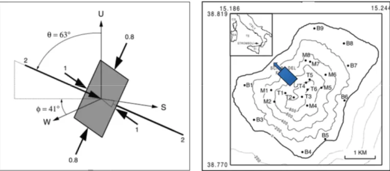
The moment tensor for a tensile crack described by the angles and Ф (Figure 2) is described by Chouet [1996] as:
Where ΔV is the volume change. If a horizontal crack is assumed, Ф is equal to zero and the tensor becomes:
If a Poisson solid is assumed, λ=µ then the eigenvalue ratio for a crack is 1:1:3. However, if a Poisson’s ratio of σ= 1/3, is more appropriate for magmatic conduit regions with low shear velocities [Chouet et al., 2003], the λ= 2μ is assumed and the ratio becomes 1:1:2.
Crack-like moment tensor ratios of around [1:1:3] and [1:1:2] have been found at several volcanoes. Different processes have been found to be responsible for the generation of VLP signals, but magma moving through an opening crack opening is the most common explanation.
Let us now consider now the radial expansion of cylinder with axis orientation given by and Ф (Figure 3). The Cartesian components of the moment tensor are:
= ΔV [λ+µ(
Ф +
Ф)] ,
= -ΔV (µ
Ф +
Ф) =
,
= -ΔV (µ
Ф +
Ф) =
,
= ΔV [λ+µ(
Ф +
Ф)] ,
= -ΔV (µ
Ф +
Ф) =
,
= ΔV (λ+µ
Ф).
Here ΔV = LΔS, where L is the pipe length and ΔS represents the increase in its cross-sectional area.
If Ф is equal to zero and the tensor becomes:
=
0
0
0
0
0 0
+ 2μ
.
Finally, the moment tensor for the spherical source (Figure 4) is given by:
=
+ 2/3μ
0
0
0
+ 2/3μ
0
0
0
+ 2/3μ
.
Where ΔV
=
Δ ,
in which R is the radius and Δ is the fractional change involume.
1.3 Example of VLP: Mt. Erebus
Strombolian eruptions from the long-lived lava lake of Erebus volcano, Ross Island, Antarctica, generate repeating Very Long Period (VLP) signals, with periods ranging between approximately 30 and 5s (Figure 5), that persist for several minutes and through the post-eruptive refilling of the lava lake. [Aster et al., 2003].
The Strombolian eruptions are initiated by a gas slug. This slug is first trapped within the conduit, presumably by a physical barrier, at a depth of no more than a few tens of meters. Once the slug breaks loose of its barrier, it rises to the surface of the lava lake, where it decompresses explosively and sprays lava and lava bombs around the crater. After the explosive eruption, the lava lake is eviscerated and begins recharging.
Figure 5. Very Long Period signals recorded on the vertical component at Mt. Erebus, associated with a strombolian eruption in December 1999. UP figure) Broadband velocity seismograms with the distance to the station shown at right. DOWN figure) Signals, integrated to displacement. (After Aster et.al 2003)
Three different groups of VLP signal types have been identified. Two types are similar and are distinguished by their initial onset polarity, being either positive or negative. The initial VLP pulse (positive or negative) also varies in timing by several seconds relative to the eruption. The remaining signal type is more pulse-like in character and very rare with only a few examples observed [Mah, 2003].
To investigate underlying forces and/or moment couples and the source location responsible for VLP signals, they use the same inversion method used to invert VLP at Stromboli Volcano, with Green's functions calculated using a 50-m resolution topographic model of the volcano using the method of using the finite-difference code (Ohminato and Chouet, 1997).
Particle motion analysis was used as a preliminary starting point for the search for the best location. A grid defines the area being considered as a possible source location. The spacing is subsequently decreased to zoom in on the areas with the best fit.
The moment rate and force rate functions determined at Erebus are consistent in some ways with results found at other volcanoes with VLP signals (Figure 6). The dominantly volumetric source with a ratio of [1.1:1:3] is consistent with the excitation of a sub horizontal crack. The initial gas bubble and subsequent mass transport exerts a pressure against the walls of the conduit. This slug is then released and rises quickly to the surface of the lava lake where it decompresses explosively, spraying the inner crater with ejecta. The volumetric expansion and contraction continues as the lava lake regains the equilibrium through an extended oscillatory mechanism. The volumetric ratio evolves slightly with time, suggesting that the process slightly deviates from a purely crack source. It remains roughly [1:1:3], through the first 60 seconds of signal, suggesting that the new magma, which has entered into the chamber to refill the conduit, also enters through the same crack.
During the lava lake recharging process, a pressure difference caused by the removal of lava lake material in the eruption will force magma to move up from a deeper reservoir into the lake reservoir. The magma is transported unsteadily, but in an oscillatory and repeatable way. The initial acceleration of magma upwards and into the lake reservoir creates a negative single vertical force rate function. The oscillatory deceleration causes the single force rate function to swing to the opposite direction. When the next pulse of magma comes from below, the process starts again, so that the result is an oscillatory single force with decreasing amplitude as the lake approaches a resumed equilibrium.
1.4 VLP at Merapi
Very-long-period (VLP) pulses with period of 6–7s, were identified in 1998 from broadband seismographs around the summit crater of Merapi Volcano. Source mechanisms for several VLP pulses were examined by applying moment tensor inversion to the waveform data (from D. Hidayat, B. Chouet, B. Voight, P. Dawson, and A. Ratdomopurbo; 2002). Merapi Volcano in central Java, Indonesia, has been characterized recently by repeated episodes of dome growth and collapse, with occasional vulcanian explosions [Voight et al., 2000a, 2000b]. In January–February 1998, four broadband seismometers were installed around the summit of Merapi. At the time, the volcano was in a phase of dome growth with seismicity characterized by multiphase (MP) earthquakes and rockfalls. The MP earthquake is an important type at Merapi, clearly associated with dome growth [Shimozuru et al., 1969; Ratdomopurbo and Poupinet, 2000; Voight et al., 2000a, 2000b], but its source mechanism is poorly understood. MP events at Merapi occur at a rate of zero up to a few events per day during times of low activity, to hundreds of events per day during periods of rapid dome growth [Ratdomopurbo and Poupinet, 2000; Voight et al., 2000b]. Most MP events during this period were accompanied by distinctive VLP waveforms [Hidayat et al., 2000]. Figure 7 shows a sample of the vertical component of 10 MP events, while Figure 8 shows the same events band-pass filtered. The repetitive action of a fixed source evidenced by the similarity of the waveforms recorded for different events.
The source locations of VLP signals at Merapi were performed by comparing the VLP particle motions produced by an isotropic point source embedded in the topography of the volcano with the observed VLP particle motions, used the finite difference (FD) code of Ohminato and Chouet [1997] to generate synthetic particle motions.
Once the source position is know, a moment tensor inversion of the observed VLP data was performed assuming a point source at the hypocenter position. The results of our inversion for moment tensor components are shown in Figure 9. The fit between the synthetic displacements and observed displacement seismograms is reasonable.
Inversions for the selected event, performed for moments tensor component only, forces component only, or both moment and forces, are all consistent with a volumetric point source with principal dipole components with ratios varying from about 0.3:1:3 to 0.6:1:3 for the three types of calculation.
Solutions were consistent with a crack striking 70° and dipping 50° SW, 100m under the active dome, suggests a pressurized gas transport involving accumulation and sudden
release of 10–60 of gas in the crack within a 6s interval.
Figure 7. (a) Amplitude normalized vertical components of velocity records showing VLP events embedded in multiphase (MP) events recorded during the 1998 experiment. The julian day, hour, and minute of each event is indicated on the right of each trace. (b) Amplitude normalized records obtained by bandpass filtering of the records in (a) in the 1–30 s band. (From D.Hidayat et al. 2002)
Figure 8.Observed (bold line) and synthetic (thin line) seismograms for a VLP pulse recorded at 14:54 UTC on 01/17/1998. The synthetic seismograms are the result of an inversion for moment tensor components only.
Figure 9. Source model obtained by inversion. The amplitude ratios for the three axe are 0.3:1:3 can be
1.5 VLP at Stromboli
Stromboli is the northernmost active volcano of the Aeolian Island arc in the Tyrrhenian sea. Following a landslide and tsunami on 30 December 2002, and paroxysmal event of 5 April 2003, Stromboli has become the focus of particular attention from the scientific community. Since January 2003, INGV (Osservatorio Vesuviano) has maintained a 13-station network of broadband seismometers on this volcano (Figure 10). Real-time data transmission allows continuous remote monitoring of Strombolian activity, consists of passive degassing (Burton et al., 2007) and intermittent, mild to moderate, Strombolian explosions (Bertagnini et al., 1999; Rosi et al., 2000; Patrick et al., 2007). These explosions usually occur from a single vent every 10–20 min on average and last between a few to 20 s, ejecting coarse materials up to a height of 100–150m that falls back to the crater terrace (Bertagnini et al.,1999). Within the range of this type of activity, the strongest explosions produce jets of magma and gas higher than 150-200 m, with material that may occasionally fall outside
the crater rims. All tephras erupted during normal explosive activity are volatile-poor scoriae fed by Highly Porphyritic (HP) magma (Francalanci et al., 1999, 2004; Corsaro et al., 2005).
The eruptive history of Stromboli is also characterized by the occurrence of more violent events that exhibit much greater explosivity with respect to the normal bursts. Barberi et al. (1993) defined two classes of powerful events based on their intensity: more frequent and less hazardous “major explosions”, and rarer and powerful “paroxysms”.
The former represent explosive events constituting a serious risk for people at the summit of the volcano, like those occurring in September 1996, August 1998 and August 1999 (Métrich et al., 2005), while the latter may represent a potential hazard also for people living or staying at the foot of the volcano. Examples of this second kind of event are the 1919 and 1930 eruptions (Ponte, 1919; Imbò, 1928; Rittmann, 1931). In addition to HP scoriae erupted during normal Strombolian explosions, large-scale paroxysms typically produce volatile-rich pumice clasts of Low Porphyritic (LP) magma (Métrich et al., 2001; Bertagnini et al., 2003; Métrich et al., 2005), as well as mingled products of the LP and HP type (Rosi et al., 2006).
VLP seismic data recorded at Stromboli Volcano have been analysed to quantify the source mechanisms and to determine the source-centroid location of typical Strombolian explosions [Chouet et al., 2003].
To determine the source location and associated mechanism we need to compare observed data to synthetic data calculated for a realistic model of volcano.
Chouet et al., (2003) obtained synthetics by using the three dimensional finite difference method of Ohminato and Chouet [1997], in which the topography and bathymetry of Stromboli are discretized in a staircase by stacking unit cells with fixed cell size (40m). Green’s functions are calculated for all the network receivers for six moment-tensor components and three single-force components applied at each source node.
Using data recorded by broadband stations, the inversion of these data has been done separately for each source node and evaluate the resulting source mechanism by computing squared errors. The best fit point source location is the position at which the residual error between data and synthetics is minimum.
The source of VLP events of Strombolian explosions was located between 220 and 260 m beneath the active vents. The source mechanisms include both moment-tensor and single-force components. The principal axes of the moment tensor have amplitude ratios [1:1:2], which can be interpreted as a crack with dip 60° to the northwest and strike northeast– southwest along a direction parallel to the “Sciara del Fuoco” (Figure 11).
Figure 11. Left) Source mechanisms. The three eigenvectors obtained from measurements of the maximum peak-to-trough amplitudes in the individual tensor components. Right) Source locations and orientations. (From Chouet et.al 2003)
The source time histories of the moment components display a characteristic sequence of inflation–deflation–inflation of the source volume (Figure 12). The initial inflation represents a pressurization of the conduit attributed to the formation and release of a slug of gas. A stronger deflation follows, which reflects the lowering of the magmastatic head associated with the rise and ejection of the slug. The next inflation marks a repressurization of the conduit caused by slumping of the liquid film surrounding the slug back to the top of the magma column after the slug has burst at the surface. The vertical force accompanying these volumetric variations is initially directed down, then up. The downward force is synchronous with the initial inflation of the source volume, while the following upward force is synchronous with the deflation of the source volume. This suggests that, initially, as the overpressured gas slug pushes the dike walls apart, it also acts piston-like to push upward the perched column of liquid above the slug. The net result of this upward acceleration of magma is an upward acceleration of the center of mass of the source volume, which induces a downward reaction force on the Earth.
Figura 12. Source time functions in which six moment-tensor components and three single-force components are assumed for the source mechanism. Shading marks the interval during which the initial volumetric expansion of the source occurs. (From Chouet et.al 2003)
1.6 VLP at other Volcanoes
Phreatic eruptions and long period tremor events at Aso volcano in Japan were inverted for locating the source and determining the focal mechanism by Legrand et al. [2000]. They found that these events were mostly volumetric, with small deviatoric components. The source was in part isotropic and in part a vertically opening crack with a volumetric tensor ratio of [3:6:1]. They also determined that a single vertical force would not be significant because these events were not correlated with large eruptions or large amounts of internal mass transport, and only gas, water, and small rocks were ever emitted from the volcano.
VLP signals associated with dome growth were observed at Merapi volcano, Indonesia [Hidayat et al., 2002]. They found a volumetric source with a ratio of around [0.3:1:3]. They obtained a better fit to their data if they included single forces in their inversion. They suggest that the source mechanism is the degassing of rising magma as it passes through cracks in the dome interior.
VLP impulsive signals were found to be associated with magma injection at Kilauea, Hawaii [Ohminato et al., 1998]. It was found that a moment tensor ratio of around [1:1:3] or [1:1:2] fit their data, depending on which stations they used. These signals were saw tooth shaped and they were explained as gated mass transport, characterized by the slow injection of a fluid into a crack and then the rapid ejection of this fluid out of the crack, corresponding to the sharp drop in the signal. They also found a significant single vertical force. They explained this force as a drag on the channel walls created by the flow of the magma through the crack.
Mount Hachijo Fuji, in Tokyo, revealed VLP signals following a volcano-tectonic (VT) earthquake swarm [Kumagai et al., 2003]. Moment tensor inversion revealed a vertical crack at a depth of 5 km as the source. No significant single forces were found. Kumagai et al. [2003] interpret their results as originating from a basalt-gas mixture resonating in a crack. The VT earthquake swarm and deformation of the island point towards magma injection which could feed the mixture into a dike.
Kumagai et al. [2001] found VLP signals associated with caldera formation at Miyake Island, Japan. The moment tensor ratio recovered for these signals was [0.7:1.2:6]. They explained the signal being generated by a piston-style mechanism which pushes magma from the chamber out through an outflow conduit.
1.7 Low-frequency events at Mt. Vesuvius
Mt. Vesuvius is a volcanic complex on the west coast of Italy, composed of an older strato-volcano, named Somma, with a summit caldera and a more recent cone (Gran Cono), which has grown inside the caldera. Its eruptive history began more than 25,000 years ago and has been characterized by large Plinian eruptions. The most famous was the eruption which destroyed the Roman towns of Pompei and Herculaneum in a.d. 79. Since that time, the largest eruption occurred in 1631 and was followed by semi-persistent activity that included several medium-sized eruptions over a period of about 300 years. This period ended with the eruption on 18 March 1944, the last eruption of Mt. Vesuvius.
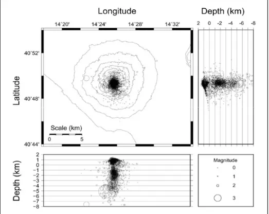
Its activity is currently characterized by moderate seismicity. The earthquake locations are highly clustered mainly localized within a radius of 3 km from the center of volcano with
depth ranging from 8 km b.s.l. to 1 km a.s.l, and magnitudes generally low (
<
3)(Figure 13) [D’Auria et al. 2013]. Although Mt. Vesuvius has been dormant since the eruption of March 1944, and shows only moderate signs of activity, its strongly explosive eruptive style, combined with nearby population centers, makes it one of the highest-risk volcanoes in the world.
Figure 13. Earthquake hypocenters for the 1999-2012 interval. The top left panel shows earthquake epicenters for events whose location uncertainty (ERH and ERZ) is less than 1 km. The size of symbols is proportional to the event magnitude (see the legend on the lower right). The plot on the left shows hypocenters projected on a NS cross-section, while the lower plot shows an EW cross-section. (Form D’Auria et al. 2013).
The seismic stations are mainly located around the volcanic edifice with a higher density in the “Gran Cono” crater area. The current configuration of the seismic monitoring network consists of 18 seismic stations and 7 infrasound microphones (Figure 14).
Figure 14. Map of Vesuvius permanent seismic monitoring network. Circles: period 1C stations; triangles: short-period 3C stations; diamonds: broadband stations; stars: strainmeters; cross: seismic array (ARV1). (From Orazi et al.2013).
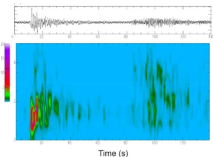
On May 11, 2012, at 01:09 UTC, the seismic network of Mt. Vesuvius recorded two low amplitude signals having atypical features [Orazi et al.,2013] (Figure 15).
Figure 15. Traces of the very-low-frequency earthquake recorded by the seismic network of Mt. Vesuvius on May 11, 2012, at 01:09 UTC. The figure shows only the vertical components (Orazi et al, 2012).
Figure 16. Spectrogram of the vertical component of the same event recorded at OVO. (From Orazi et al.2013).
In the past, long-period events, have been already identified at Vesuvius [Bianco et al. 2005], but the signals recorded now, have waveforms and spectra differing from those of typical LP events [Chouet 1996].
The first event has clear P and S seismic phases. This allowed the determination of the event hypocentre, which was located below the volcanic edifice, West of the cone, at a depth of about 1.36 km b.s.l. The P wave polarities were compatible with a double couple mechanism. The main signal was followed, about 70 s later, by another signal having a more complex waveform but a similar spectrum. This second signals seems to consist in the superposition of many small events, having the same waveform of the first one.
The low value of the computed stress drop, less than 0.1 bar, suggests a source mechanism different from typical VT earthquakes. This kinematics is similar to that of slow earthquakes, which are usually recorded along convergent plate boundaries [Ide at al. 2007].
Similar events to these were also recorded and study on other volcanoes: Mount Etna,
Turrialba Volcano in Costa Rica and Ubinas Volcano in Peru [Christopher J. Bean et
al.,2013]; in this work they use a numerical model to show that slow-rupture failure in unconsolidated volcanic materials can reproduce all key aspects of these observations. Therefore, contrary to current interpretations, they suggest that short-duration long-period events are not direct indicators of fluid presence and migration, but rather are markers of deformation in the upper volcanic edifice. They suggest that long-period volcano seismicity forms part of the spectrum between slow-slip earthquakes and fast dynamic rupture, as has been observed in non-volcanic environments.
2 Methods
2.1 Green’s Function.
We first developed a procedure to compute the amplitude and phase of the wave field made by a source of low-frequency events in an arbitrary volcanic structure. Our purpose was to model the full wave field of these events considering a complex topography. We used the Finite Element Method (FEM) to compute the Green’s functions in the Fourier domain. This choice has been justified by the fact that the elastodynamic Green’s Functions are written as elliptic equations in the Fourier domain and the FEM is a suitable technique to solve elliptic problems. This method is particularly well suited when the boundary condition have some complex geometries.
2.2 Finite elements method (FEM)
The physical domain.
The first thing we have to define is the geometry of the computational domain (Figure 17).
For instance in we are given a polygon Ω. Its boundary is a closed polygonal curve Г.
The boundary of the polygon, Г, is divided into two parts,which do not overlap over the whole domain:
• The Dirichlet boundary Г , • The Neumann boundary Г .
On the Dirichlet boundary displacements are given while on the Neumann boundary normal stresses are given.
Green’s Theorem
The approach to solve this problem above with the Finite Element Method is based upon writing it in a different form, which is called the weak or variational form. The most important theorem in this process or reformulating the problem is the Green’s Theorem, one the most popular results of vector calculus. Sometimes it is also called Green’s First Formula. The theorem states that:
,
note that there are two types of integrals in this formula. Both integrals in the left-hand side
are domain integrals in Ω, whereas the integral in the right-hand side is a line integral on
the boundary Г. The result is also true in three dimensions. In that case, domain integrals are volume integrals and boundary integrals are surface integrals. The dot between the gradients denotes simply the Euclidean product of vectors, so:
The weak form
The starting point for defining the weak or variational formulation is Green’s Theorem. Here it is again:
Note that we have parted the integral on Г as the sum of the integral over the two sub-boundaries, the Dirichlet and the Neumann boundary. Now we substitute what we know in this formula: we know that Δu = f - cu in Ω and that = on Г . Therefore, after some rearrangements:
Note now that we have written all occurrences of u on the left hand side of the equation
except for one we have left on the right. In fact we don’t know the value of on that part
of the boundary:
v = 0. on Г therefore:
We have not imposed yet the Dirichlet boundary condition ( u = on Г ).
Nevertheless, we have imposed a similar one in the function v , but in a homogeneous way. As written now, data ( f and ) are in the right-hand side and coefficients of the equation (the only one we have is c ) are in the hand side. The expression on the left-hand side is linear in both u and v. It is a bilinear form of the variables u and v. The expression on the right-hand side is linear in v.
Without specifying spaces where u and v are, the weak formulation can be written as follows:
for all v , such that v = 0 on Г .
Note how the two boundary conditions appear in very different places of this formulation:
1) The Dirichlet condition (in our case this means: given displacements) is imposed apart from the formulation and involves imposing it homogeneously to the testing function . It is called an essential boundary condition.
2) The Neumann condition (given normal stress) appears inside the formulation. It is called a natural boundary condition.
The discrete variation problem
The finite element method (with finite elements on polygons) consists of the following discrete version of the preceding weak formulation:
We have done three substitutions:
1) We look for the unknown in the space instead of the whole Sobolev space. This
means that we have reduced the problem in computing in the vertices of the
triangulation (in the nodes) and we are left with a finite number of unknowns.
2) We have substituted the Direchlet condition by fixing the values of unknowns on Dirichlet nodes. This reduces the number of unknowns of the system to the number of free nodes.
3) Finally, we have reduced the testing space from Г ( ) to its discrete subspace Г .
We will show right now that this reduces the infinite number of tests of the week formulation to a finite number of linear equations.
The associated system
We write again the discrete problem, specifying the numbering of Dirichlet nodes in the discrete Dirichlet condition:
Our next claim is the following: the discrete equations
are equivalent to the following set of equations:
Obviously, this second group of equations is a small part of the original one: it is enough to
take = ∈ Г .. Recapitulating, the method is equivalent to this set of N
equations to determine the function :
Then we substitute the discrete Dirichlet condition in this expression:
Finally we plug this expression in the discrete variational equation:
We consider the linearity, noticing that:
and move to the right-hand side what we already know (the Dirichlet data):
This is a linear system with a many equations as unknowns, namely with
= Г equations and unknowns. The unknowns are in fact the nodal values of
on the free (non-Dirichlet) vertices of the triangulation. After solving this linear system,
The wave equation
We will use homogeneous Dirichlet conditions in the entire boundary of the domain. The wave propagation problem is then:
If we use the finite difference approach, the simplest thing to do is to apply the central difference approximation to the second derivative. If we consider a fixed time step, this means approximating:
When applied to the time-variable in the wave equation we obtain the explicit time-step
After considering the weak formulation and introducing finite element spaces and bases, we end up with:
The initial value for is easy. We still need to determine . We first take a Taylor approximation:
or take a false discrete time -1 and use the equation:
to obtain the equation:
2.3 Example computation
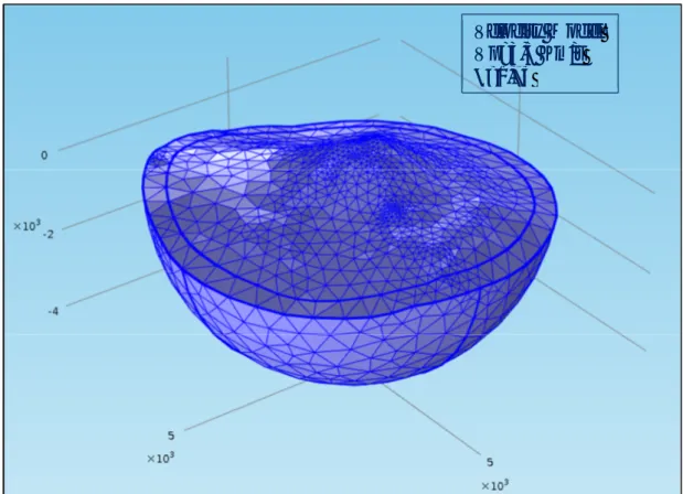
Green’s functions have been calculated in the frequency domain, through a three-dimensional finite element method using the simulation software «COMSOL Multiphysics». We have imposed PML (Perfect Matched Layers) boundary conditions on the edges of the model.
The discretized model, including the topography of Stromboli, has been done using an irregular tetrahedral mesh. The maximum elements size was chosen based on the minimum wavelength, related to the maximum frequency used (3Hz). The velocity model
consists in a homogeneous medium with compressional wave velocity =3,5 Km/s and
/ =√3 (Chouet et al., 2003).
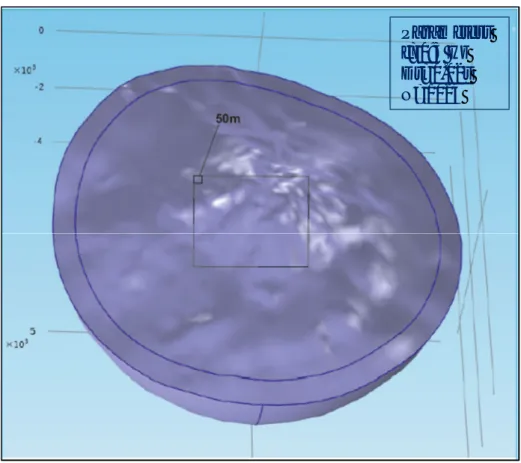
For our purpose, the Green’s functions are obtained for individual point sources positioned on grid nodes spaced 50 m apart. The black square in figure indicates the surface projection of the selected computational domain extending up to 1 km depth.
As shown by Auger et al. [2006], a dramatic reduction in computation times is achieved by using the reciprocal relation between source and receiver [Aki andRichards,1980]:
where the Green's function (r,s) expresses the n-component of displacement at r due to
a unit impulse applied in the i-direction at s. Using reciprocity, the three components of displacement can be calculated at each source node for impulsive forces applied in the x, y and z directions at each stations of the network.
1) Definition of the computational volume
∙ = 0
u= 0
Velocity Model
Vp=3,5 Km/s =1,73
2) Discretized Model of Stromboli
Figure 19. Surface projection of the selected computational domain Parameters f=0:3 Hz Dt=0.02s N=1024
3) Computational domain
This model has been developed considering two boundary conditions: 1) Neumann’s condition, which imposes the cancellation condition of the normal stress at the free surface and the Dirichlet’s condition on the external boundary of the computational domain where the displacement over the surface is zero. We have used this latter condition because we need to ensure stability to the solution. Anyway, this condition is appropriate to model the wavefield, because it decays before arriving to the external edge, being damped by the Perfect Matched Layers (PML).
The PML is an additional domain where the elastodynamic equations are changed to get an exponential decay of the waves in a particular direction. We choose a spherical model where the direction of the decay is radial.
Below we show the results of Green’s Function calculated for the Mxx component of the moment tensor at 1 Hz of frequency (Figure 20.)
2.4 The source inversion method: traditional approaches
Once Green’s functions are known, we can calculate synthetic seismograms based on a model and see how well they fit the observed seismograms.
In this work we considered a point source since the signal wavelength is much greater than the distance between the source and receiver. The displacement field generated by a seismic source can be described by the representation theorem, which for a point source, can be expressed through the convolution [Chouet, 1996; Ohminato et al., 1998; Chouet et al.,2003, 2005]:
( ) = ( ) ∗
( ) +
( ) ∗
,( )
where the first term (zero-order) represents the single force while, the second term
(first-order) represents the moment tensor components and is the Green’s function
corresponding to each moment tensor and single force component. The proportion of moment tensors as dictated by the moment rate functions (Figure 21) should tell us valuable information about the eruptive process. Earthquakes are often well described by double couple sources. As earthquake sources have a pure shearing motion component and no volume change, their moment tensors is dominated by the deviatoric components. Thus, when modelling earthquakes, the moment tensor is constrained to have a null trace to account for the purely deviatoric component. From Figure it can be seen that the tensor elements along the diagonal of the tensor control volumetric changes while the off-diagonal (deviatoric) tensor elements control shear motions. This figure also illustrates the reason for the symmetry of the moment tensor. For typical earthquake sources, six moment tensor elements considered can be reduced to 5 if it is assumed that there is no volume change, and this can be reduced to just three in the case of a planar fault [Lay and Wallace, 1995].
However, for volcanic settings, taking into account of changes in volume of the seismic sources is usually required, because volcanic processes involve expanding gases and motion of magma, thus necessitating the inversion of all six double couple components.
The signals seen at Stromboli are due to implosive or explosive forces associated with the buoyant transport and decompression of a bubble of gas within a magma conduit and to subsequent mass transport. Therefore, volumetric forces are likely to dominate the moment rate tensor solutions at Stromboli, so that volumetric components are likely to be much larger than deviatoric ones.
Also, due to the movement and eruption of material, there may be linear momentum that are not completely balanced internally by the Earth, at least in the frequency band observed here. Instead of just the moment tensor mechanism represented in Figure, there could also be single force components (e.g. [Kanamori et al., 1984], [Chouet et al., 2003], [Ohminato et al., 1998]).
The inversion of source mechanisms can be performed either in the time or in the frequency domain.
The classic approach [Uhira and Takeo, 1994; Ohminato et al., 1998; Chouet et al., 2003, 2005] considers the convolution relation in the time domain:
Discretization of the integral in this equation usually leads to a very large square matrices whose dimension represents the product of the number of generalized moment components, , times the number of time steps, , used in the convolution operation. As each element of this matrix is itself obtained through a time consuming convolution, the computation of the matrix lasts more than the matrix inversion.
Auger at al. (2006) have shown that frequency domain methods allow a quick inversion of the source allowing a real-time computation:
( ) = ( )
( ) +
( )
,( )
Unconstrained frequency-domain inversionIn the previous equation, the signal is represented as a single force and a moment tensor component multiplied with their respective Green’s functions.
Being a linear problem, its solution can be easily obtained using a least squares approach, solving a system of 9 equations for each frequency. This constitutes an important advantage over similar techniques. On the other hand it requires a high number of degrees-of-freedom (9 for each frequency component), making results poorly reliable when dealing with a limited number of operating seismic stations (i.e. less than 5) and/or noisy recordings.
2.5 Constrained inversion
In order to limit the number of degrees of freedom (DOF) associated with the inverse problem, making the procedure more stable, our strategy is to constrain the geometry of the source mechanism to be constant during the event and to vary only in its magnitude. This reduces the number of DOF to 2 for each frequency with 9 more DOF for the source mechanism geometry. In our approach the displacement field generated by a seismic source is:
( ) =
( )
( ) +
( )
,( )
Constrained frequency-domain inversionWhere are the single force components, are the moment tensor components and
, are the Green’s Functions.
The source functions, under this constrain, are only two: one for the single force ( ) and
another for the moment tensor component ( ). However the problem formulated under
this constrain is non-linear and must be solved using linearized iterative approaches as the Levenberg-Marquardt. In our approach, we first determine a preliminary source function by using a Monte Carlo method, and then we use this preliminary solution to start the iterative procedure. The reduction in the number of DOF makes the procedure more reliable when used with noisy signals and/or with a limited number of stations.
2.6 The Levenberg-Marquardt method
The Levenberg-Marquardt method is a standard technique used to solve non-linear least squares problems. Ordinary least squares problems arise when fitting a parameterized function to a set of measured data by minimizing the sum of the squares of the errors between the data and the function. Non-linear least squares problems arise when the function is non-linear in its parameters. Non-linear least squares methods involve an iterative improvement of parameter values in order to reduce the sum of the squares of the errors between the function and the measured data points. The Levenberg-Marquardt curve-fitting method is actually a combination of two minimization methods: the gradient descent method and the Gauss-Newton method:
∆ =
inv(
+
(
))
∆
Levenberg-Marquardtwhere
∆
is the perturbation vector, J is the Jacobian,is the damping and
∆
is theresidual vector.
Small values of the algorithmic parameter ε result in a Gauss-Newton update and large values of ε result in a gradient descent update. The parameter ε is initialized to be large.
If an iteration results in a worse approximation, ε is increased. As the solution approaches
the minimum, ε is decreased, the Levenberg-Marquardt method approaches the
Gauss-Newton method, and the solution typically converges rapidly to the local minimum.
Like all the iterative linearization algorithms, also the LM method needs having an initial test solution, to start the iterative procedure. In our case it was chosen as the initial solution that obtained by the linear inversion of a source with isotropic moment tensor M and vertical single force F (M=[1:1:1] F=[0:0:1]). This is motivated by the fact that usually the moment tensor component of seismo-volcanic events is usually dominated by a volumetric component, while the single force, being often associated with explosion, is generally sub-vertical.
3 Synthetic Tests
The new constrained inversion method has been tested over a synthetic dataset, reproducing realistic VLP signals of Stromboli Volcano using the actual seismic network
configuration of Stromboli (see Figure 22).In the synthetic tests we assess our capability
to retrieve the source time function and mechanism when different signal-noise ratio is added to the data (S/N from 2 to 200) in a different seismic network configurations (12 stations (ALL), 5 summit stations (TOP), 5 random stations (MIX). The location of the test source is fixed.
.
The characteristics of the test sources have been chosen to mimic actual sources observed at Stromboli, both in terms of waveform shape and amplitude. The test source mechanism is not isotropic and the single force is purely vertical (M=[3:2:1] F=[0:0:1]). (Figure 23)
The fit of synthetics waveforms to the observed ones was computed according to the misfit function:
Where is the data trace, is the synthetic trace and N is the numbers of samples in
each traces.
The Figure 24, 25 and 26 shows the waveforms matches between linear inversion (blue line) and new constrained inversion (red line) for different signal/noise ratios and the same network configurations (ALL). The black line is the waveform of source test.
Figure 23. Source time function test for moment tensor (magnitude: ∗ N*m) and single force (magnitude: )
Figure 24. Waveform match obtained, in which six moment-tensor components and three single-force components are assumed for the source mechanism. The red lines indicate the constrained inversion solutions, the blue lines indicate unconstrained linear inversion solutions and black lines indicate waveform source test. “ALL” configurations and S/N=200.
Waveforms Test
Waveforms Linear inversion
Wave form Constrained inversion
Figure 25. Waveform match obtained, in which six moment-tensor components and three single-force components are assumed for the source mechanism. The red lines indicate the constrained inversion solutions, the blue lines indicate unconstrained linear inversion solutions and black lines indicate waveform source test. “ALL” configurations and S/N=10.
Waveforms Test
Waveforms Linear inversion
Wave form Constrained inversion
Figure 26. Waveform match obtained, in which six moment-tensor components and three single-force components are assumed for the source mechanism. The red lines indicate the constrained inversion solutions, the blue lines indicate unconstrained linear
inversion solutions and black lines indicate waveform source test. “ALL” configurations and S/N=2. Waveforms
Test
Waveforms Linear inversion
Wave form Constrained inversion
Observing the Figures 27, 28 and 29 it is evident that, by comparing the waveforms obtained from the two inversions method, with those relating to the source 'test', the linear unconstrained inversion shows the best results going from S/N=200 to S/N= 2 for the same network configuration.
Figure 27. Waveform match obtained, in which six moment-tensor components and three single-force components are assumed for the source mechanism. The red lines indicate the constrained inversion solutions, the blue lines indicate unconstrained linear inversion solutions and black lines indicate waveform source test. “ALL” configurations and S/N=10.
Waveforms Test
Waveforms Linear inversion
Wave form Constrained inversion
Figure 28. Waveform match obtained, in which six moment-tensor components and three single-force components are assumed for the source mechanism. The red lines indicate the constrained inversion solutions, the blue lines indicate unconstrained linear inversion solutions and black lines indicate waveform source test. “MIX” configurations and S/N=10.
Figure 29. Waveform match obtained, in which six moment-tensor components and three single-force components are assumed for the source mechanism. The red lines indicate the constrained inversion solutions, the blue lines indicate unconstrained linear inversion solutions and black lines indicate waveform source test. “TOP” configurations and S/N=10.
Waveforms Test
Waveforms Linear inversion
Wave form Constrained inversion
Waveforms Test
Waveforms Linear inversion
Wave form Constrained inversion
To summarize the results, on the Figure 30 we represent the misfit function for different network configurations and different S/N ratios for both the constrained and the unconstrained inversion. It is evident how the misfit function for the unconstrained inversion is systematically lower that the constrained one. This can be easily explained considering the higher number of degrees of freedom (DOF) of the unconstrained linear inversion (9*Nf) compared to constrained inversion (9+2*Nf).
WaveformTest
Waveform Linear Inversion Waveform Constrained Inversion
On the other hand, the comparison of the quality of the retrieved results in terms of time source function shows that the performances of the constrained inversion are superior for low S/N and for all the considered network geometries (Figure 31 and 32). In particular, the best results are more evident in the case of reconstruction of the three components of single force.
*
m m
Figure 31. Source time functions fit, in which six moment-tensor components and three single-force components are assumed for the source mechanism. Network configurations is “ALL”.
WaveformTest
Waveform Linear Inversion Waveform Constrained Inversion
*
m
Figure 32. Source time functions fit, in which six moment-tensor components and three single-force components are assumed for the source mechanism. Different network configurations.
In the Figure 33 we represent the norm of the difference between the retrieved and the true source functions for both single force and moment tensor components.
For the moment tensor component, the constrained inversion results are better for S/N ratios lower than about 10, for ALL and TOP configurations, and lower than 50 for the MIX configuration. Similar values are found for the single force component.
Eigenvectors determined for the moment tensor solutions of the synthetic test are shown in Figure 34. The better performances of the constrained inversion (red line), are clear. For low S/N ratio and/or sparse network configuration, the unconstrained inversion (blue line) gives erroneous results, while performances of the constrained inversion are still good.
3.1 Source locations
The results of synthetic tests have been obtained with a known location of the source. Since the inversion of the source mechanism requires accurate Green’s functions, it is necessary first to locate the centroid of the event in order to get a reliable mechanism. We perform the location using a probabilistic approach based on the computation of a normalized probability function over a regular grid (see Figure 35). The probability distribution function can be used to get the maximum-likelihood location estimator as well as the confidence ellipsoid using a standard probabilistic approach.
N
We calculated the misfit function for every point of the regular grid:
Using a probabilistic approach, to assess the location quality, we have:
The probability function then is normalized, so we have:
Misfit Function
Probability Function
Below we show two example locations for a good (200) and a very poor (2) S/N ratio using all the 12 available stations. In the former case the retrieved source is very close to the actual position and the confidence ellipsoid has a maximum length of about 200 m. The thick green line indicates the isoline enclosing 50% of probability. In the latter, the source has been located about 150 m below the true position and the probability density function is spread over a wide area.
N
N
Probability
Figure 36. Representation of the probability distribution. Configuration ‘ALL’ S/N =200
Probability N
N
4 Stromboli dataset
The Stromboli volcano erupted on February 27, 2007, after about two months of intense Strombolian activity. The eruption was characterized by a sequence of rapidly evolving phenomena: the propagation of an effusive fracture along the crater rim, the opening of lateral effusive vents, an unusually large effusive flux (> 10 m3/s), the collapse of the crater system, and a violent Strombolian explosion.
We show that the constrained inversion method was able to correctly invert the seismic source of VLP events at Stromboli, and to determine the location and the geometry.
Therefore we have selected a VLP event on February 18, at 4:38, recorded by the seismic broadband network (Figure 38). The seismograms are characterized by explosion signals superimposed on a sustained background of tremor.
Figure 39 shows the same record as in Figure 38 band-pass filtered between 0.2 and 0.05 Hz with a 2-pole zerophase-shift Butterworth filter. This record enhances the VLP components present in the explosion signals from 0 to 20 s.
Figure 38. Seismic signals of explosion event on February 18, at 4:38, recorded by the broadband seismic network of Stromboli N-S E-W V STR1 STR4 STR5 STR6 STR8 STR9 STR3 STRA STRB STRC STRD STRE
Figure 39. 20 s selected window for the same seismic signal as for Figure 38 band-pass filtered between 0.5 and 0.02Hz STR1 STR4 STR5 STR6 STR8 STR3 N-S E-W V STR9 STRA STRB STRC STRE STRD Time(s)
To determine the source-centroid location we apply the probabilistic approach illustrated in sec. 3.1.
Figure 40. Representation of the probability distributions for the VLP centroid location
Figure 40 illustrates the probability distributions calculated for the selected VLP event. It spreads over a limited volume and the confidence ellipsoid has a maximum length of about 300 m. The source centroid of the VLP event is located approximately 200 m beneath of the active vents, on “Sciara del Fuoco”, where the persistent activity of the volcano occurs. Figure 41 shows the waveform matches obtained by the unconstrained linear inversion and the constrained inversion technique. As seen in synthetic tests, unconstrained inversion shows in this case the best results.
The fit is computed for all the stations in operation at the time, and for a source mechanism consisting of six moment tensor and three single-force components.
Figure 41. Calculated (red line) and observed seismograms (black line) are compared for the unconstrained inversion of the explosion that occurred on the 18th February 2007 at 4:38
STR1 STR4 STR5 STR6 STR8 STR3 N-S E-W V STR9 STRA STRB STRC STRE STRD Time(s)
STR1 STR4 STR5 STR6 STR8 STR3 N-S E-W V STR9 STRA STRB STRC STRE STRD Time(s)
Figure 42. Calculated (red line) and observed seismograms (black line) are compared for the constrained inversion of the explosion that occurred on the 18th February 2007 at 4:38
The source time functions associated with the best fit model depicted in Figures 41 and 42 are shown in Figures 43 and 44, respectively. The results are consistent with what we expect about the dynamic of seismic source at Stromboli, on the basis of previous studies. The volumetric components of the moment tensor clearly dominate in each solution. Accompanying the volumetric source components there is a dominantly vertical force. Observing the figures it is possible to note that the results obtained by the constrained inversion are of better quality. We have shown that the solution for moment tensor components is relatively stable, appears less affected by the noise both in terms of moment tensor but especially for the single components of the force, compared to the unconstrained linear inversion.
In Figure 45 we show the source mechanisms obtained for the selected events. The black lines are the eigenvectors obtained from the unconstrained linear inversion. The amplitude ratios of the principal axes of the moment tensor are quite stable although there is greater scatter in the directions of the eigenvectors respect to the constrained inversion (red line). A T-k plot (after Hudson et al.1989) showing source mechanism types for the moment tensor solutions obtained from two inversions. T (horizontal axis) is a measure of the deviatoric component in the source. k (vertical axis) is a measure of the isotropic (volume change) component. A DC (Double-Couple) and a CLVD (Compensated Linear Vector Dipole) are purely deviatoric (k=0) mechanisms. An explosion is a purely isotropic (T=0) mechanism. All red points of unconstrained inversion solutions are concentrate into two areas between Tensile Crack and Explosion while the solution of constrained inversion is located near the explosion mechanism.
Figure 45. Source mechanisms obtained for the selected event. The reference coordinates for the eigenvectors are EW (east– west), NS (north–south), and UD (up–down). (a) Plot of eigenvectors for the moment-tensor solution obtained for unconstrained (black line) and constrained inversion (red line). (b) “Hudson Plot”.
EW NS UD Unconstrained Inversion Constrained Inversion a) b)
5 Vesuvius dataset
On May 11, 2012, at 01:09 UTC, the seismic network of Mt. Vesuvius recorded low frequency seismic event having peculiar features (Figure 46).
CMDT POB VBKN VCRE VTIR OVO
Figure 46. Vertical component of the low-frequency earthquake recorded by the seismic network of Mt. Vesuvius on May 11, 2012, at 01:09 UTC. The stations selected are only those equipped with broadband sensors. The signals were filtered with pass band between 0.5-2s. (From Orazi et al. 2013)
In particular the possibility of identifying the first arrivals of the P and S phases on the seismogram allowed to locate the event hypocenter which was below the volcanic edifice, West of the cone, at a depth of about 1.36 km b.s.l, and the P wave polarities analysis were compatible with a double couple mechanism (Figure 47).
Figure 47.Focal mechanism and epicenter location of the low-frequency event. (From Orazi et al.2013)
We have used the new constrained inversion to study this particular event and we have compared the result with the unconstrained linear inversion, as seen in the previous case of Stromboli.
Calculated and observed data are compared in Figures 48 and 49, for the two type of inversions.
Figure 48. Calculated (red line) and observed seismograms (black line) are compared for the waveform unconstrained inversion of the low frequency that occurred on May 11, 2012, at 01:09 UTC.
Figure 49. Calculated (red line) and observed seismograms (black line) are compared for the waveform constrained inversion of the low frequency that occurred on May 11, 2012, at 01:09 UTC.
In the Figure above we present the results obtained by the unconstrained inversion while below, in the second figure those related to the new constrained inversion. As already seen in synthetic tests and the dataset of Stromboli, unconstrained linear inversion shows better quality results for all stations. But always as seen before, the reconstruction of the source time function in terms of the moment tensor is always more stable and better quality in the case of the constrained inversion. In particular by observing the results obtained by both methods it is clear that the low frequency event recorder is characterized by a more complex source mechanism, not associated to a pure double couple. In fact is possible to observe that in the Hudson diagram, by plotting the source mechanism for both types of inversion, red points are furthest from the center of the graph (pure DC). Therefore by the results obtained our idea is that this low-frequency events, recorded at Vesuvius, are linked to slow earthquakes that have origins, in shallow depth of volcano, in the ductile zone.
Figure 50. Source mechanisms obtained for the event selected. (Left) Plot of eigenvectors for the moment-tensor solution obtained for unconstrained (black line) and constrained inversion (red line). (Right) “Hudson Plot”.
Unconstrained Inversion Constrained Inversion
6 Conclusion
The aim of this thesis was to develop, test and apply a novel method for the inversion of seismo-volcanic events. The study of low frequency seismo-volcanic signals, recorded by broadband seismic networks, is important in understanding the dynamics on volcanic systems with special reference to volcano monitoring and eruption forecasting. For this reason different inversion techniques have been developed . In particular, the main topic of this thesis is the development and the validation of new constrained non-linear inversion technique of the of low frequency seismo-volcanic signals, aimed at determining the location and the geometry of the source and its dynamics. The development of this method has been motivated by the needs of inverting the seismic source function in conditions of low signal/noise ratios and a limited number of recordings.
The waveform inversion has been performed in the frequency domain. In order to limit the number of degrees of freedom (DOF) associated with the inverse problem, our strategy has been to constrain the source mechanism to be constant during the event, varying only in its magnitude. This constrain reduces the number of DOF to 2 for each frequency with 9 more DOF for the source mechanism geometry. This significantly reduces the number of parameters to invert, making the procedure more stable in a reduced network configuration and a low signal-noise ratio respect to other inversion methods. The problem formulated under this constrain is non-linear and must be solved using linearized iterative approaches as the Levenberg-Marquardt.
The method has been tested over a synthetic dataset, reproducing realistic Very-Long-Period signals of Stromboli Volcano, using different signal-noise ratios, in different seismic network configurations.
To locate the centroid of the source we follow a probabilistic approach based on the computation of a probability density function over a regular grid. The probability distribution function can be used to get the maximum-likelihood location estimator as well as the confidence ellipsoid using a standard statistical approach.
Tests were performed comparing our inversion method with linear unconstrained inversions. The results of the test shows that the linear unconstrained inversion shows the best results. This can be easily explained considering the greater number of DOF of the unconstrained linear inversion (9*Nf) compared to constrained inversion (9+2*Nf), with Nf being the number of frequencies used in the inversion.