UNIVERSITY
OF
BERGAMO
F
ACULTY OF
E
CONOMICS AND
B
USINESS
A
DMINISTRATION
R
ESEARCH
D
OCTORATE IN LOGISTICS AND SUPPLY CHAIN
MANAGEMENT
D
OCTORAL THESIS
ACHIEVING
MULTIPLE-PERFORMANCE
EXCELLENCE
THROUGH
LEAN
MANUFACTURING:
EMPIRICAL EVIDENCES USING CUMULATIVE
AND TRADE
-
OFF MODELS
S
UPER VISOR
:
P
H
.D.
C
ANDIDATE
:
2
INDEX
1 INTRODUCTION………..1
1.1 Research questions ... 1
1.2 Structure of the thesis and methodology adopted ... 6
1.3 Data collection ... 7
1.4 References ... 8
2 CUMULATIVE MODEL FOR LEAN MANUFACTURING………11
2.1 Introduction ... 11
2.2 Literature review and hypotheses ... 14
2.2.1 Lean Manufacturing ... 14
2.2.2 Operational Performance ... 17
2.2.3 In defense of the sand cone model... 17
2.2.4 Links between Lean Manufacturing and the sand cone model ... 19
2.3 Methodology ... 22
2.3.1 Measurement of variables ... 22
2.3.1 Content validity ... 23
2.3.2 Unidimensionality, reliability, convergent and discriminant validity of the measurement variables ... 24
2.3.3 Structural model results ... 30
2.4 Discussion ... 34
2.5 Conclusions ... 36
2.6 References ... 38
Appendix A ... 42
3 TRADE-OFF MODEL: ASSESSING THE IMPACT OF JUST-IN-TIME ON OPERATIONAL PERFORMANCE AT VARYING DEGREES OF REPETITIVENESS……….55
3
3.1 Introduction ... 55
3.2 Literature review and theoretical framework ... 58
3.3.1 Characteristics of non-repetitive manufacturing contexts ... 59
3.3.2 Just-in-time ... 61
3.3.3 Just-in-time and operational performance ... 62
3.3.4 Interaction effects on performance ... 63
3.4 Methodology ... 66
3.4.1 Data collection ... 66
3.4.2 Measures ... 66
3.4.3 Measurement model ... 68
3.4.4 Structural equation modeling results ... 71
3.5 Discussion ... 73
3.6 Conclusions and limitations ... 76
3.7 References ... 77
APPENDIX A ... 83
APPENDIX B ... 86
4 A SECOND TRADE-OFF MODEL: JIT-PRODUCTION, JIT-SUPPLY AND PERFORMANCE, INVESTIGATING THE MODERATING EFFECTS………88
4.1 Introduction ... 88
4.2 Literature review and hypotheses ... 90
4.2.1 JIT practices ... 91
4.3 Methodology ... 97
4.3.1 Data collection and sample ... 97
4.3.2 Variables and measurement scale assessment ... 99
4.3.3 Hierarchical regression and expert analysis ... 103
4
4.5 Discussion and implications ... 110
4.6 Conclusions ... 115 4.7 References ... 117 Appendix A ... 122 Appendix B ... 124 5 CONCLUSIONS………128 References ... 132
1
1 INTRODUCTION
The intensification of global competition and the crisis have forced manufacturing companies to explore all available opportunities for reducing their costs without compromising the other operational performance. As a consequence, there has recently been renewed attention towards Lean Manufacturing. This attention doesn’t come only from managers, but also from academics.
This thesis has the main purpose to understand the mechanism by which manufacturing companies could achieve multiple-performance excellence through the implementation of Lean Manufacturing.
To obtain this objective I adopted one cumulative model and two trade-off models to empirically demonstrate how Lean Manufacturing could improve operational performance and to highlight possible problems and traps when implementing Lean Manufacturing practices in particular contexts and configurations.
1.1
Research questions
What is Lean Manufacturing? Shah and Ward (2007) defined Lean Manufacturing as a “methodology that aims at eliminating waste by reducing supplier, internal and
customer variability through an integrated socio-technical system that involves the simultaneous use of many practices”.
Starting with this definition, the preliminary step of a empirical research on Lean Manufacturing is to operationalized it into a measurable scale.
Bearing in mind that to make significant academic contributions it is important to study a phenomenon using a commonly accepted and comprehensive measurement scale (McCutcheon and Meredith, 1993), in scientific literature it is possible to note that
2
Lean Manufacturing is often confused with other methodologies (for example with Just-In-Time, a methodology that is part of Lean Manufacturing, but it doesn’t cover all the facets of Lean Manufacturing methodology) and it is measured with a multitude of different scales, thus limiting academic and managerial contributions of previous academic researches (Shah and Ward, 2007).
Since in scientific literature there is a lack of a well defined and comprehensive Lean Manufacturing measurement scale, the first research question that this thesis wants analyze and answer is:
RQ 1: what are the Lean Manufacturing practices that a
comprehensive measurement scale must consider to make relevant
theory advancement?
Going beyond this problem, Shah and Ward (2007) argued that “the relationships
among the elements of Lean Manufacturing are neither explicit nor precise in terms of causality”.
This statement makes clear that in scientific literature there is a lack of empirical evidences about causality relations and interconnection between Lean Manufacturing practices.
This academic gap arises a managerial problem because it is impossible to understand the right implementation sequence of Lean Manufacturing practices without a strong knowledge about causal relationships between these practices.
The importance of filling this gap is given by John et al. (2001) because they told us that an implementation sequence that builds manufacturing capabilities is fundamental if the purpose of a manufacturing company is to have a sustaining competitive advantage, since it is not possible to concentrate all the efforts to introduce a new manufacturing methodology at the same time (Skinner, 1969).
For this reason, the second research question is:
RQ 2: are Lean Manufacturing practices causal related? How?
Why?
3
Moreover, most of the empirical studies concerning Lean Manufacturing analyzed the impact of some Lean Manufacturing practices on operational performance measured as a single construct that includes at the same time multiple dimensions (e.g. McKone et al., 2001; Furlan et al., 2011) with the result that it is not clear to what extent the Lean Manufacturing practices can improve individual performance dimensions.
Furthermore, there are empirical studies that operationalized the performances with multiple constructs for multiple dimensions, but without any causal relation between them (e.g. Flynn et al., 1995; Cua et al., 2001; Shah and Ward, 2003; Li et al., 2005).
However, we know that a lot of models about sequence of operational performance dimensions exist in scientific literature (e.g. the sand cone model about cumulative capabilities: Ferdows and De Meyer, 1990). These models, even though are very famous, they are also criticized and not yet effectively proved (Flynn and Flynn, 2004, Rosenzweig and Easton, 2010).
From the abovementioned discussion, a third gap of the literature is a lack of a comprehensive study about the relationships between Lean Manufacturing practices and each operational performance dimension and a fourth gap is the lack of empirical evidences about sequence of performance dimensions (quality, delivery, flexibility and cost).
Thus, this thesis aims at answering to the following two research questions:
RQ 3: how does Lean Manufacturing improve operational
performance? Why?
RQ 4: how are operational performances related? Why?
These first four research questions will be answered by the paper presented in Chapter 2 where I will prove that Lean Manufacturing practices help to dramatically improve operational performances if manufacturing companies follow a precise sequence of implementation to build cumulative capabilities.
4
From the cumulative model results presented in Chapter 2 may seem that Lean Manufacturing methodology could be universally adopted to obtain maximum results on operational performances.
However, there could be contingent variables or unexplored synergies between practices that lead to trade-off results on performance (e.g. Efficiency vs. Responsiveness).
The two trade-off models presented in Chapters 3 and 4 aim at analyzing these potential effects.
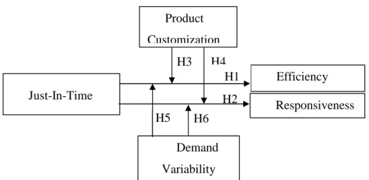
In literature almost all of successful lean stories came from repetitive contexts, where products are standardized and customer demand is stable and predictable (product customization and demand variability represent the contingent variables) (Jina et al., 1997; Lander and Liker, 2007).
The most critical Lean Manufacturing bundle of practices in non-repetitive contexts is Just-In-Time, mainly because demand fluctuations make takt time dynamic and the high product variety inhibits production smoothing (Lander and Liker, 2007; Reichhart and Holweg, 2007).
Just-In-Time practices were firstly developed in Toyota, where the production is highly repetitive, and for many years researchers have thought that this methodology could be applied in contexts characterized by repetitive manufacturing systems only.
Recently some authors have refuted this view, providing empirical evidences that Just-In-Time practices can be successfully implemented also in non-repetitive contexts. However, these evidences came from descriptive and anecdotal case studies, whereas in the literature, studies based on large sample lack, which analyze Just-In-Time impact on performance at varying degrees of repetitiveness.
Thus, the gap of the literature is the lack of a study based on a large sample, which analyze Just-In-Time impact on performance at varying degrees of repetitiveness.
The fifth research question is as follows:
RQ 5: is Just-In-Time applicable in non-repetitive manufacturing
contexts? In particular: how the contingent variables that represent
5
the degree of manufacturing repetitiveness could affect the positive
impact of Just-In-Time on operational performances?
This research question will be answered by the paper presented in Chapter 3 where I will demonstrate that Just-In-Time could be also applied in non-repetitive contexts as long as the variability of the customer demand not exceed a certain value.
As regards the possible synergies between Lean Manufacturing practices, even though the vast majority of researchers argues that Lean Manufacturing in general, and Just-In-Time specifically, dramatically improve operational performances, in literature it is possible to find some authors supporting a lack of significant relationships between some Just-In-Time practices and performance (e.g. Sakakibara et al., 1997; Dean and Snell, 1996; Flynn et al., 1995).
Mackelprang and Nair (2010) argued that the potential (and still unexplored) existence of moderating effects between Just-In-Time practices (e.g.: Just-In-Time manufacturing and Just-In-Time supply) could be an explanation for the contrasting results on the link between Just-In-Time and performance.
As a consequence, in scientific literature there is a lack of empirical evidences about synergies between JIT practices that are part of the Lean Manufacturing methodology.
Thus, the last research question of this thesis is as follows:
RQ 6: is there a moderating effect between Just-In-Time
manufacturing and Just-In-Time supply that could lead to possible
trade-offs on operational performances?
This research question will be answered by the paper presented in Chapter 4, where I will demonstrate that Just-In-Time supply positively moderates the relationship between Just-In-Time manufacturing and delivery performance and this effect lead to trade-off between efficiency and delivery performances in particular Just-In-Time manufacturing – Just-In-Time supply configurations.
6
1.2
Structure of the thesis and methodology adopted
The thesis is composed by three papers that are organized as follows: after a introduction about the specific research, I will present the literature review and, consequently, the theoretical model definition, after that I will describe the methodology adopted. Finally a discussion of the main results will conclude each chapter.
At the end of the thesis, in Chapter 5, I will summarize the academic and managerial contributions in relation with the research questions discussed in this chapter.
The empirical research of this thesis is based on survey methodology. To test the cumulative and trade-off models, I have followed a common structure in all the three papers:
1. Content validity of the variables of interest
2. Confirmatory Factor Analysis to test the measurement model a. Standardization of the data by country and industry
b. Assessment of unidimensionality, convergent validity and reliability for the all of the first-order constructs
c. Discriminant validity for the first-order constructs assessed by conducting a series of χ²difference tests between nested models for all pairs of constructs
d. Convergent validity for the second-order constructs (for the cumulative model)
e. Discriminant validity for the second-order constructs (for the cumulative model)
3. Test of the hypotheses with different methods, depending on the specific purpose
a. Structural Equation Modeling for the cumulative model (Chapter 2) b. Structural Equation Modeling and Ping (1995)’s 2-step approach to
test the moderating hypotheses of the first trade-off model (Chapter 3)
7
c. Hierarchical regression method to test the moderating hypotheses of the second trade-off model (Chapter 4)
In every chapter I decided to use slightly different tests to demonstrate my knowledge about the survey methodology, nevertheless trying to keep the methodology discussion lean and easy to read.
1.3
Data collection
I use data from the third round of the High Performance Manufacturing (HPM) project data set (Schroeder and Flynn 2001). The survey questionnaire was distributed by my research group in collaboration with an international team of researchers working in different universities all over the world to a selection of plants from different countries (i.e. Finland, US, Japan, Germany, Sweden, Korea, Italy, Austria, China and Spain). These countries were included because they contain a mix of high performing and traditional manufacturing plants in the selected industries, while providing diversity of national cultural and economic characteristics.
The selected plants operate in machinery (SIC code: 35), electronics (SIC code: 36) and transportation components (SIC code: 37) sectors. As I said before, the plants were randomly selected from a master list of manufacturing plants in each of the countries. Within the research group, for each country, a group of researchers and a person in charge of plant selection process and data collection were identified. Each local HPM research team used different tools for selecting plants. In Italy, we used Dun’s Industrial Guide.
The study administrators sent requests to each local HPM research team to include an approximately equal number of high performing and traditional manufacturing plants. This allowed to include in the sample plants that use advanced practices in their industry, i.e. World Class Manufacturing (WCM) plants, as well as traditional (i.e. not
8
WCM) plants. Finally, all plants had to represent different parent corporations, and have at least 100 employees.
The questionnaire was firstly developed in English, then was translated into the local language by the local research team. Informants were selected based on their skills and expertise on the topic investigated.
Each plant received a batch of questionnaires targeted at the respondents who were the best informed about the topic of the specific questionnaire. In order to reduce the problem of common method bias, each questionnaire was administered to different respondents within each plant.
Researchers involved in HPM project asked the CEOs (or to a coordinator within each plant) to provide us with the name and contact addresses of the respondents for each questionnaire, and to distribute the questionnaires received by individual visits or by post to the respondents.
Each local HPM research team had to provide assistance to the respondents, to ensure that the information gathered was both complete and correct.
1.4
References
Cua, K.O., McKone, K.E. and Schroeder, R.G., 2001. Relationships between implementation of TQM, JIT, and TPM and manufacturing performance. Journal of
Operations Management. 19(6), pp. 675-694.
Dean, J.W. and Snell, S.A., 1996. The strategic use of integrated manufacturing: an empirical examination. Strategic Management Journal. 17(6), pp. 459-480.
Flynn, B.B., Sakakibara, S. and Schroeder, R.G., 1995. Relationship between JIT and TQM: practices and performance. Academy of Management Journal. 38(5), pp. 1325-1360.
Ferdows, K. and De Meyer, A., 1990. Lasting improvements in manufacturing performance: In search of a new theory. Journal of Operations Management. 9(2), pp. 168-184.
9
Flynn, B.B. and Flynn, E.J., 2004. An exploratory study of the nature of cumulative capabilities. Journal of Operations Management. 22(5), pp. 439-457.
Furlan, A., Dal Pont, G. and Vinelli, A., 2010. On the complementarity between internal and external just-in-time bundles to build and sustain high performance manufacturing. International Journal of Production Economics, Article in Press, DOI: 10.1016/j.ijpe.2010.07.043.
Jina, J., Bhattacharya, A.K. and Walton, A.D., 1997. Applying lean principles for high product variety and low volumes: Some issues and propositions. Logistics
Information Management, 10(1), pp. 5-13.
John, C.H.S., Cannon, A.R. and Pouder, R.W., 2001. Change drivers in the new millennium: implications for manufacturing strategy research. Journal of Operations
Management. 19(2), pp. 143-160.
Lander, E. and Liker, J.K., 2007. The Toyota Production System and art: Making highly customized and creative products the Toyota way. International Journal of
Production Research, 45(16), pp. 3681-3698.
Li, S., Rao, S.S., Ragu-Nathan, T.S. and Ragu-Nathan, B., 2005. Development and validation of a measurement instrument for studying supply chain management practices. Journal of Operations Management. 23(6), pp. 618-641.
Mackelprang A.W. and Nair, A., 2010. Relationship between just-in-time manufacturing practices and performance: A meta-analytic investigation. Journal of
Operations Management. 28. pp. 283-302.
McCutcheon, D. and Meredith, J.R., 1993. Conducting case study research in operations management. Journal of Operations Management. 11(3), pp. 239-256.
McKone, K.E., Schroeder, R.G. and Cua, K.O., 2001. The impact of total productive maintenance practices on manufacturing performance. Journal of Operations
Management. 19(1), pp. 39-58.
Ping, R.A., 1995. A parsimonious estimating technique for interaction and quadratic latent variables. Journal of Marketing Research, 32(AUGUST), pp. 336-347.
Reichhart, A. and Holweg, M., 2007. Creating the customer-responsive supply chain: a reconciliation of concepts. International Journal of Operations and Production
10
Rosenzweig, E.D. and Easton, G.S., 2010. Tradeoffs in Manufacturing? A Meta-Analysis and Critique of the Literature. Production and Operations Management. 19(2), pp. 127-141.
Sakakibara, S., Flynn, B.B., Schroeder, R.G. and Morris, W.T., 1997. The impact of just-in-time manufacturing and its infrastructure on manufacturing performance.
Management Science, 43(9), pp. 1246-1257.
Shah, R. and Ward, P.T., 2003. Lean manufacturing: Context, practice bundles, and performance. Journal of Operations Management. 21, pp. 129-149.
Shah, R. and Ward, P.T., 2007. Defining and developing measures of Lean Manufacturing. Journal of Operations Management. 25(4), pp. 785-805.
11
2 CUMULATIVE MODEL FOR LEAN
MANUFACTURING
4.1
Introduction
Lean Manufacturing (LM) is a methodology that involves the simultaneous use of many techniques and tools. Shah and Ward (2003) have developed the measurement scale of LM, identifying four bundles of practices: Just-In-Time (JIT), Total Quality Management (TQM), Human Resource Management (HRM) and Total Productive Maintenance (TPM). In Operations Management (OM) scientific literature LM is defined either as a philosophy that follows strategic principles, such as continuous improvement and waste reduction, or a set of practices, like kanban, cellular manufacturing and so on (Shah and Ward, 2007). To make significant academic contributions it is important to study a phenomenon using a commonly accepted and comprehensive measurement scale (McCutcheon and Meredith, 1993). However, there are very few studies that have investigated LM holistically, causing a problem of generalizability of the results. One of the studies that analyzed LM holistically is Shah and Ward (2007). Shah and Ward (2007) defined LM as “an integrated socio-technical
system whose main objective is to eliminate waste by concurrently reducing or minimizing supplier, customer, and internal variability”. The authors argued that LM
could be viewed in a configurational perspective, since LM practices seems to be inter-related but not clearly causal inter-related, thus LM practices are complementary and synergic rather than sequential, and only the concurrent use of the all set of LM practices leads to a competitive advantage (Shah and Ward, 2007).
From the abovementioned discussion arises a managerial problem. Indeed, the creation of a strategy that builds manufacturing capabilities following a precise sequence of practices is vital to obtain maximum results and a sustaining competitive advantage (John et al., 2001). As a matter of fact, it is not possible to implement at the
12
same time all the manufacturing practices, since managers typically don’t have sufficient resources (Skinner, 1969; Rosenzweig and Easton, 2010). For this reasons, managers need an implementation sequence of tools and techniques that could maximize the impact of these practices on operational performances.
A research stream (Cua et al., 2001; McKone et al., 2001; Furlan et al., 2011), tried to fill this gap studying some causal relationships between LM practices, however these studies firstly didn’t analyze together all LM practices and secondly they didn’t differentiate the impact of LM on the different dimensions of operational performance. The first problem causes a lack of generalizability of the results, while the second leads to possible errors of implementation sequence of manufacturing capabilities. It is fundamental to study sequence of practices – or manufacturing capabilities – implementation in relation to a precise sequence of operational performance achievement – or competitive capabilities – (Ferdows and De Meyer, 1990). Ferdows and De Meyer (1990) used the “sand cone” model to describe how a manufacturing company could build a sustainable success through a cumulative sequence of capabilities. In particular, the authors stated that manufacturers have to focus on manufacturing capabilities that are able to improve quality (quality conformance), after that on capabilities for quality and dependability (delivery performance), then for quality, dependability and speed (flexibility performance) and finally also for cost reduction.
Starting from the seminal publication of Ferdows and De Meyer (1990), some researchers have studied the relationship between these performance dimensions (e.g. Noble, 1995; Boyer and Lewis, 2002; Flynn and Flynn, 2004; Rosenzweig and Roth, 2004; Großler and Grubner, 2006).
Noble (1995) analyzed through a exploratory survey, based on regression and cluster analyses, the strategies and priorities of 561 companies in North America, Europe and Korea and found out that the manufacturing strategy follows a sequence of priorities that starts from quality, then dependability, delivery, cost, flexibility and innovation.
Boyer and Lewis (2002) studied 110 plants that had implemented Advanced Manufacturing Technologies (AMT) to understand if there are evidences of trade-off between priorities. The authors argued that manufacturers and decision makers need to
13
set priorities in trade-off, even though the use of AMT guide to cumulative capabilities effects.
Flynn and Flynn (2004) used multiple regression analysis to test in 165 plants located in five countries and operating in three industries whether cumulative capability sequences are country and industry specific. Empirical evidences of this study didn’t support the generalizability of the “sand cone” model, since the sequence of capabilities changed for different countries. In addition, the authors argued that manufacturing strategies support the foundation of cumulative capabilities, while they don’t for the high-level parts of capabilities.
Rosenzweig and Roth (2004) gave empirical evidences of the “sand cone” model, confirming the sequence of Ferdows and De Meyer (1990) on a restricted sample of 81 plants and explain how manufacturing capabilities lead to business profitability.
Großler and Grubner (2006) proposed an alternative path model to test the accuracy of cumulative capabilities. They assumed that after the sequence of quality and delivery capabilities, delivery has a direct impact on both flexibility and cost, while these capabilities are modeled in trade-off. After a Structural Equation Modeling procedure on a sample of 558 plants operating in 17 countries and 5 industries, the authors concluded that the cumulative part of their theoretical framework is valid, thus quality results as the baseline of the model, followed by delivery capability. Results of this research suggest also that after delivery, companies could improve simultaneously cost and flexibility capabilities. Finally, results cannot support the trade-off nature of cost-flexibility relationship.
From the abovementioned studies, it can be found a substantial agreement on the first two competitive capability dimensions sequence of the “sand cone” model, namely quality and delivery performance, while there is no an universal agreement on the sequence of the last two dimensions: flexibility and cost.
These mixed results could be explained by several argumentations and problems. First of all, there is no consensus about the measures to test the “sand cone” model, as a matter of facts, some authors measured competitive priorities instead of competitive capabilities (Flynn and Flynn, 2004; Rosenzweig and Easton, 2010). The second problem is connected with the sample size: when the sample is restricted, the generalizability of the results is limited. Another problem is the theoretical framework
14
of reference and the methodology adopted: the analysis of the simple path of competitive capabilities without a comparison of rival models is too limited to assert that an a priori model is acceptable. Moreover, when a theoretical framework refers to manufacturing strategies and their link with competitive capabilities, structural equation modeling has to be preferred in comparison to multiple regression analysis because the latter methodology can’t test at the same time all the theoretical framework; this problem goes against fit theory, that requires the presence of all the variables of interest in the same structural model, to verify the different contribution of manufacturing capabilities on competitive capabilities, and at same time test the “sand cone” model.
The aim of this chapter is twofold. On the one hand to give empirical evidences about causality relations and interconnection between LM practices, on the other to propose a cumulative sequence of LM capabilities based on a comprehensive study about the relationships between LM practices and each operational performance dimension and relationships between performances, thus testing the “sand cone” model. As a matter of facts, in this chapter, I consider not only how LM practices are linked together and can affect operational performance, but also how they can trigger a series of performance improvements according to the sequence suggested by Ferdows and De Meyer’s (1990) model.
4.2
Literature review and hypotheses
2.2.1
Lean Manufacturing
Shah and Ward (2007) define Lean Manufacturing as a methodology that aims at eliminating waste by reducing supplier, internal and customer variability through an integrated socio-technical system that involves the simultaneous use of many practices. The authors point out the importance of studying LM using commonly accepted and comprehensive measurement scales to make significant academic contributions. Indeed, for example, LM is often confused with Just-In-Time (JIT), while JIT is only a sub-set
15
of LM practices, and this leads to misalignments between theory and empiricism. To solve this problem Shah and Ward (2007) developed the LM measures, identifying ten distinct dimensions: supplier feedback, JIT delivery by suppliers and supplier development (supplier related constructs); customer involvement (customer related construct); pull, continuous flow, set up time reduction, total productive maintenance, statistical process control and employee involvement (internally related constructs). These LM dimensions could be grouped following four bundles of practices, named: Just-In-Time (JIT), Total Quality Management (TQM), Human Resource Management (HRM) and Total Productive Maintenance (TPM) (Shah and Ward, 2003).
Even though Shah and Ward (2007) have argued that “the relationships among the
elements of Lean Manufacturing are neither explicit nor precise in terms of linearity or causality”, it is possible to find a stream of literature that studied the causality relations
and interconnection between LM practices. Cua et al. (2001) revealed the importance of using TQM, JIT and TPM practices simultaneously to maximize operational results, supported by McKone et al. (2001) who theorized that JIT and TQM alone cannot improve operational performance, but they act as mediators between TPM and operational performance, in fact TPM practices on the one hand they facilitate the introduction of TQM because reduce process variability, on the other they help JIT because increase plant capacity.
Furlan et al. (2011) distinguish two parts of the LM system, the technical part, represented by JIT and TQM tools, and the social part, represented by HRM practices. The authors have proved that JIT and TQM are complementary and HRM acts as an antecedent and enabler that creates the right environment where develop the technical part of the system. As a matter of fact, the combination of TQM and JIT creates additional complexity and makes worker training and skills more important (Snell and Dean, 1992), thus, the implementation of JIT and TQM requires an adequate organizational change because “technology alone does not provide companies with
better performance” (Challis et al., 2005). Aihre and Dreyfus (2000) argued that the
success of the introduction of new quality improvement programs depends not only on the employee’s knowledge and training, but also on a coherent manufacturing strategy. This is due to the fact that a clear manufacturing strategy, based on a continuous improvement foundation, is able to direct all the efforts toward new technical and
16
managerial directions (Hayes and Wheelwright, 1988). Finally, this manufacturing strategy must be shared with suppliers carefully selected to reinforce the relationship with them, and it must be aligned with the company business strategy to achieve maximum firm results (Flynn et al., 1995; Swink et al., 2005).
Actually, all the aforementioned TPM tools and human and strategic oriented practices (see Table 2.1) are common to both JIT and TQM methodologies. This common set of practices is named in literature Infrastructure (Flynn et al., 1995).
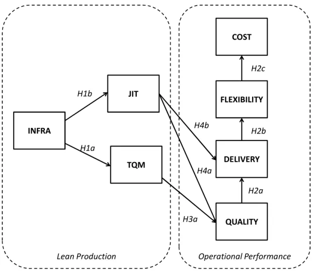
Based on these considerations, I argue that LM is composed by three main bundles: Infrastructure, JIT and TQM, that are related as follows:
H1a: The Infrastructure is an antecedent of TQM H1b: The Infrastructure is an antecedent of JIT
Table 2.1: Lean Manufacturing practices
Bundles Practices
JUST IN TIME Daily Schedule Adherence
Flow Oriented Layout JIT links with suppliers Kanban
Setup Time Reduction TOTAL QUALITY MANAGEMENT Statistical Process Control
Process Feedback
Top-Management Leadership for Quality Customer Involvement
Supplier Quality Involvement
INFRASTRUCTURE Total Preventive / Autonomous
Maintenance Cleanliness
Multi-Functional Employees Small Group Problem Solving
17
Employee Suggestions
Manufacturing-Business strategy linkage Continuous Improvement
Supplier Partnership
2.2.2
Operational Performance
Most of the empirical studies concerning LM analyzed the impact of LM practices on operational performance measured as a single construct that includes at the same time multiple dimensions (e.g. quality, delivery, flexibility and cost) (McKone et al., 2001; Tan et al., 2007; Furlan et al., 2011) or as multiple constructs for multiple dimensions without any causal relation between them (Flynn et al., 1995; Cua et al., 2001; Shah and Ward, 2003; Li et al., 2005). These approaches lead to several problems: using a single construct could generate difficulties in interpreting results because it is impossible to distinguish the contributions on each dimension of performance, while missing causal relationships between performance dimensions decreases the explanatory power of the model and influence the interpretation of the results about the real impact of LM practices on performance.
To solve these problems, this research uses the perspective of the sand cone model (Ferdows and De Meyer, 1990), a very famous model about sequence of cumulative capabilities, but still criticized and not yet effectively proved (Flynn and Flynn, 2004, Rosenzweig and Easton, 2010).
2.2.3
In defense of the sand cone model
Quality conformance represents the baseline of the cumulative sequence described in the sand cone model (Ferdows and De Meyer, 1990; Flynn and Flynn, 2004). Quality conformance is recognized as the most important competitive capability to develop (White, 1996) and the precursor of all the other competitive capabilities – delivery, flexibility and cost – (Schmenner and Swink, 1998) as it builds a stable foundation for
18
the other competitive capabilities improvements because it makes the production system more stable through a reduction of process variance (Ferdows and De Meyer, 1990). This reduction improves delivery performance because cycle times are shortened by speeding product throughput, thus allowing improved schedule attainment and faster response to market demands (Flynn and Flynn, 2005). Indeed, if quality conformance is high, it is possible to control lead time variances, since rework diminishes (Flynn and Flynn, 2004) and consequently the material moves quickly through the production process.
For these reasons, cycle time is more predictable (Flynn et al., 1999) and the outcome of the process (time and quality) is less uncertain (Schmenner and Swink, 1998), allowing more reliable production scheduling and delivery dates (Rosenzweig and Roth, 2004).
H2: Quality conformance is the baseline of the sand cone model H2a: Quality conformance directly improves delivery
Increasing delivery performance through a better knowledge about the production process and a reduction of cycle times improves flexibility (Ferdows and De Meyer, 1990) because the time required to respond to variations in customer demand decreases, thus it is easier to adjust internally production processes, following the changed requirements (Grobler and Grubner, 2006).
If the throughput time is not under control, a company is not sufficiently able to meet the customer demand, and the consequence of this lack of demand reliability is reflected in a worse flexibility capability. Only starting with a delivery improvement (also thanks to a closer relationship with the customer and coordination with suppliers that diminishes demand variability) it is possible to improve flexibility (Rosenzweig and Roth, 2004).
H2b: Delivery directly improves flexibility
Flexibility is the ability of changing production volume and mix following the customer demand without safety stocks (Jack and Raturi, 2002) and with little time or
19
cost penalties (Swink et al., 2005). Consequently, flexibility diminishes the need of inventory buffers that negatively affect cost performance, such as overproduction and obsolete finished products (Avella et al., 2011), having a direct and positive effect on cost (Rosenzweig and Roth, 2004).
On the contrary, delivery is not directly connected with cost reduction because a company could be reliable by using large amounts of inventories, thus producing with extra costs (Schmenner and Swink, 1998). Cost is reduced only if flexibility becomes a routine (Adler et al., 1999) and it represents the most difficult capability to reach, because only when all the other capabilities are improved it is possible to focus on cost reduction (Ferdows and De Meyer, 1990), since cost doesn’t influence any other capability, but it is influenced by them (White, 1996).
H2c: Flexibility directly improves manufacturing cost
2.2.4 Links between Lean Manufacturing and the sand cone model
In the first part of the literature review I hypothesized that Lean Manufacturing is composed by three bundles, and that Infrastructure acts as an antecedent of JIT and TQM. In the second part I sequenced the competitive capabilities. In the last part I connect these two parts of the framework depicted in Figure 2.1 to determine how Lean Manufacturing builds its competitive advantage.
TQM methodology includes unique practices that are not shared with JIT. These practices are: Statistical Process Control, Process Feedback, Top-Management Leadership for Quality, Customer Involvement and Supplier Quality Involvement (Flynn et al., 1995; Cua et al., 2001; Shah and Ward, 2003; Prajogo and Sohal, 2006). These TQM unique practices provide tools and approaches for solving quality problems in the production system. The adoption of TQM practices decrease process variability through a reduction of scraps and reworks and the primary outcome of the adoption of TQM practices is a product without defects (Flynn et al., 1995), thus:
20
H3a: TQM directly improves quality conformance
Even though the primary determinant of TQM is quality conformance, TQM practices indirectly improve also delivery, flexibility and cost through the reduction of manufacturing process variance. The use of TQM unique practices has a positive effect on cycle times and delivery reliability because they reduce the number of item produced and the dimension of the lot size. This reduction is due to the fact that TQM unique practices decrease the need of cycle and safety stocks, since they improve the work flow constancy and precision (Flynn et al., 1995).
Delivery performance improves not only for the reduced manufacturing process variance, but also because the presence of suppliers involved in quality efforts permits to reduce the time needed for quality inspections and permits to have supplies more reliable and flexible (Romano, 2002).
The delivery improvements obtained by the concurrent use of TQM unique practices have a positive effect on flexibility, because the increased capability to produce with reduced lead time and lot sizes, permits to have manufacturing processes synchronized with the customer demand without the use of inventories (Work-In-Progress and final products) (Flynn et al., 1995). Thus, also cost improves because there is less need of inventories to protect the production system against external variance (Sim and Curtola, 1999).
H3b: TQM indirectly improves delivery, flexibility and manufacturing cost through quality conformance in accordance with the sand cone model sequence
JIT methodology includes unique practices that are not shared with TQM. These practices are: Daily Schedule Adherence, Flow Oriented Layout, JIT links with suppliers, Kanban, Setup Time Reduction (Shah and Ward, 2003; Shah and Ward, 2007; Mackelprang and Nair, 2010; Furlan et al., 2011).
JIT methodology aims at producing the right quantity of products at the right time (delivery reliability). However, JIT improves not only delivery time, but also reduces the variance in quantity and quality of the production processes (Green et al., 2005).
21
Indeed JIT, by reducing lot sizes, reduces scraps, reworks and failures, improving quality.
JIT directly improves quality conformance because the reduction of inventory reduces the risk of handling damage, reduced lot sizes decreases the number of defects if the process goes out of control, since, with large lot sizes, quality controls are made later and with a higher possibility of defects (Flynn et al., 1995). Thus,
H4a: JIT directly improves quality conformance H4b: JIT directly improves delivery
JIT, with the introduction of a pull system, permits a closer match between production and customer demand, improving delivery performance. JIT indirectly improves also flexibility: in order to perfectly match the demand, a pull system reduces lot sizes and setup times and uses a little extra capacity to meet unexpected demand and to be more reliable, and through these improvements, also flexibility improves (Flynn et
al., 1995).
Moreover, for a pull system it is important to maintain a closer relationship with suppliers to obtain more frequent deliveries to meet the final customer demand. These deliveries not only improve delivery performance, but also flexibility, since the amount of material delivered every time is reduced (reduced inbound lot size) (Sim and Curatola, 1999).
When delivery and flexibility are met, then also costs could be reduced because it is possible to eliminate WIP and final goods inventories (Flynn et al., 1995; Sim and Curatola, 1999). JIT is more than a reduction inventory program. Flexibility is improved and inventories are reduced as the result of a better quality, lead time and delivery performance (Sim and Curatola, 1999; Fullerton et al., 2003). For this reason,
H4c: JIT indirectly improves delivery, flexibility and manufacturing cost through quality conformance and delivery in accordance with the sand cone model sequence
22 Operational Performance Lean Production INFRA JIT TQM COST FLEXIBILITY DELIVERY QUALITY H1a H1b H2a H2b H2c H3a H4a H4b
Figure 1: theoretical framework
2.3
Methodology
2.3.1 Measurement of variables
This study uses data from the third round of the High Performance Manufacturing (HPM) project data set. The analyses are based on a sample of 317 manufacturing plants, settled in several countries around the world (i.e. Finland, US, Japan, Germany, Sweden, Korea, Italy, Austria, Spain and China), and operating in machinery,
23
electronics and transportation component sectors. The questionnaires used in the present research are a subset of the whole HPM survey. Respondents within each plant were specifically asked to give answers on Infrastructure, Just-In-Time and Total Quality Management practices adopted and performance obtained.
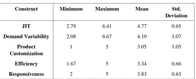
All the items comprising Infrastructure, Just-In-Time and Total Quality Management constructs were developed from Likert-scaled items, with values ranging from 1 (“strongly disagree”) to 7 (“strongly agree”). As to the items composing the operational performance constructs, we asked respondents to provide their opinion about plant’s performances compared with its competitors on a 5 point Likert scale (1 is for “poor, low” and 5 is for “superior”).
In the literature review section I defined LM as a methodology that includes Infrastructure, Just-In-Time and Total Quality Management. I conceptualized these bundles as second-order factors and measured through distinct first-order factors, corresponding to the associated practices, while each practice was measured with a multi-item scale.
2.3.1 Content validity
An extensive literature review has allowed to select the items that cover all important aspects of each practice, thus ensuring content validity (Nunnally, 1978). The scales included in this chapter are adaptations of existing and commonly used scales in OM literature.
The variables of interest that refers to the Lean Manufacturing bundles (Infrastructure, Just-In-Time and Total Quality Management) were conceptualized as second-order constructs.
Infrastructure was measured including all the common practices shared by JIT and TQM methodologies (Flynn et al., 1995), such as Total Preventive Maintenance (Cua et
al., 2001; McKone et al., 2001); cleanliness, multi-functional employees, small group
problem solving and employee suggestions, which represent the HRM practices (Snell and Dean, 1992; Aihre and Dreyfus, 2000; Challis et al., 2005; Furlan et al., 2011), manufacturing-business strategy linkage (Hayes and Wheelwright, 1988; Flynn et al.,
24
1995; Swink et al., 2005), Continuous Improvement (Hayes and Wheelwright, 1988), Supplier Partnership (Flynn et al., 1995; Swink et al., 2005).
Just-In-Time was measured with five first-order constructs, namely: daily schedule adherence (Flynn et al., 1995; Cua et al., 2001; Ahmad et al., 2003; Mackelprang and Nair, 2010; Furlan et al., 2011) , flow oriented layout (Sakakibara et al., 1997; Ahmad
et al., 2003; Shah and Ward, 2003; Shah and Ward, 2007; Mackelprang and Nair, 2010;
Furlan et al., 2011), JIT links with suppliers (Sakakibara et al., 1997; Ahmad et al., 2003; Shah and Ward, 2007; Mackelprang and Nair, 2010), kanban (Flynn et al., 1995; Sakakibara et al., 1997; Ahmad et al., 2003; Shah and Ward, 2003; Shah and Ward, 2007; Mackelprang and Nair, 2010; Furlan et al., 2011) and setup time reduction (Sakakibara et al., 1997; Ahmad et al., 2003; Shah and Ward, 2003; Shah and Ward, 2007; Mackelprang and Nair, 2010; Furlan et al., 2011).
Total Quality Management was measured with five first-order constructs: statistical process control (Flynn et al., 1995; Sakakibara et al., 1997; Cua et al., 2001; Shah and Ward, 2003; Shah and Ward, 2007), process feedback (Flynn et al., 1995; Sakakibara et
al., 1997; Cua et al., 2001; Ahmad et al., 2003), top-management leadership for quality
(Flynn et al., 1995; Sakakibara et al., 1997; Cua et al., 2001), customer involvement (Flynn et al., 1995; Sakakibara et al., 1997; Cua et al., 2001; Ahmad et al., 2003; Shah and Ward, 2007) and supplier quality involvement (Flynn et al., 1995; Sakakibara et al., 1997; Cua et al., 2001; Shah and Ward, 2003; Shah and Ward, 2007).
With regard to operational performance, I used four first-order constructs, following the dimensions of Ferdows and De Meyer (1990)’s model: quality conformance and cost were measured as a single item scale, while delivery and flexibility as a two item scales (for details see Appendix A).
2.3.2 Unidimensionality, reliability, convergent and discriminant
validity of the measurement variables
To analyze the structural model and test our hypotheses, the items of each Infrastructure, JIT and TQM practice measure were parceled with the aim at reducing
25
the complexity of the model and to meet the minimum sample size required for structural equation modeling analysis.
For each practice, I computed a single indicator that corresponds to the average of the items’ responses. This procedure was adopted in different and important studies in OM literature (e.g. Cua et al., 2001; Sila, 2007).
However, before the analysis of the structural model, I conducted a complete Confirmatory Factor Analysis (CFA) to verify if the second-order factor measurement model was valid and reliable.
I used LISREL 8.80 to perform the CFA. Even if Flynn and Flynn (2004) argued that there are different patterns of cumulative capabilities for different countries and industries, I want to test whether the sand cone model (Ferdows and De Meyer, 1990) is the best sequence of competitive capabilities and if it could be generalized. For this reason, before the CFA, I standardized data by country and industry, since they could affect the measurement and structural models results (Flynn et al., 1990).
Moreover, an iterative modification process permitted to refine the scales and to assess the unidimensionality for the first and second-order constructs. The iterative modification process was conducted to improve the parameters and fit statistics of the construct model. Indeed, when the recommended parameters were not respected, I eliminated one item at time (Joreskog and Sorbon, 1989), until the model parameters were met. If a construct had less than 4 items, the iterative modification process was conducted on a two-constructs model, where the second construct was used as a common basis of reference to have sufficient degrees of freedom to compute fit statistics (Li et al., 2005). Appendix A reports the details about the items and the iterative modification process adopted.
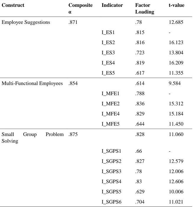
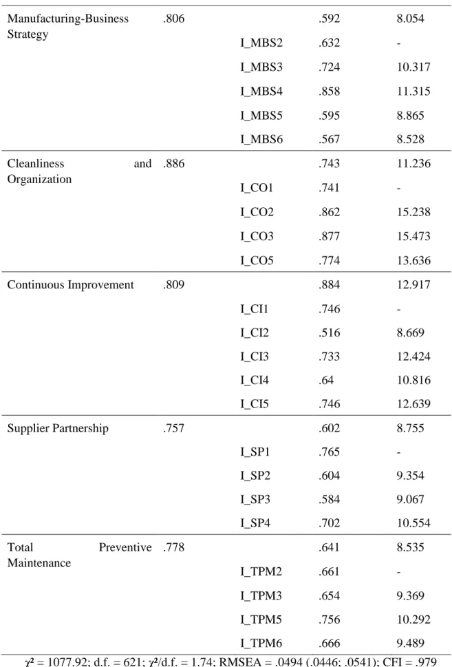
After the iterative modification process, I assessed the model fit for the three Lean Manufacturing bundles of practices. For each bundle, I verified the overall model fit, analyzing absolute (RMSEA), incremental (CFI) and parsimonious (χ²) indices. All fit indices are above the recommended cutoff points, indicating that the measurement model is acceptable (see Table 2.2, 2.3 and 2.4).
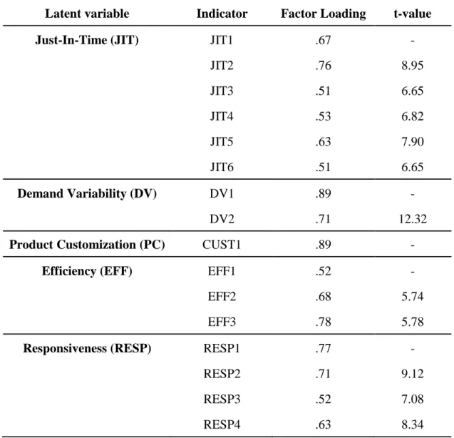
Convergent validity for the first-order constructs is demonstrated when all factor loadings of the observable variables on their first-order latent construct are statistically significant, and, similarly, convergent validity for the second-order constructs is assured
26
when all factor loadings of the first-order latent constructs on their second-order latent construct are statistically significant (Anderson and Gerbing, 1988).
Convergent validity is assured since all factor loadings of the first and second order constructs are significant at 0.01 level and greater than 0.50. Table 2.2, 2.3 and 2.4 report all factor loadings, t-values and fit indices of the measurement model.
Table 2.2: Infrastructure factor loadings, t-values and fit indices (part A)
Construct Composite α Indicator Factor Loading t-value Employee Suggestions .871 .78 12.685 I_ES1 .815 - I_ES2 .816 16.123 I_ES3 .723 13.804 I_ES4 .819 16.209 I_ES5 .617 11.355 Multi-Functional Employees .854 .614 9.584 I_MFE1 .788 - I_MFE2 .836 15.312 I_MFE4 .829 15.184 I_MFE5 .644 11.450
Small Group Problem Solving .875 .828 11.060 I_SGPS1 .66 - I_SGPS2 .827 12.579 I_SGPS3 .78 12.006 I_SGPS4 .83 12.606 I_SGPS5 .629 10.006 I_SGPS6 .704 11.021
27
Table 2.2: Infrastructure factor loadings, t-values and fit indices (part B) Manufacturing-Business Strategy .806 .592 8.054 I_MBS2 .632 - I_MBS3 .724 10.317 I_MBS4 .858 11.315 I_MBS5 .595 8.865 I_MBS6 .567 8.528 Cleanliness and Organization .886 .743 11.236 I_CO1 .741 - I_CO2 .862 15.238 I_CO3 .877 15.473 I_CO5 .774 13.636 Continuous Improvement .809 .884 12.917 I_CI1 .746 - I_CI2 .516 8.669 I_CI3 .733 12.424 I_CI4 .64 10.816 I_CI5 .746 12.639 Supplier Partnership .757 .602 8.755 I_SP1 .765 - I_SP2 .604 9.354 I_SP3 .584 9.067 I_SP4 .702 10.554 Total Preventive Maintenance .778 .641 8.535 I_TPM2 .661 - I_TPM3 .654 9.369 I_TPM5 .756 10.292 I_TPM6 .666 9.489 χ² = 1077.92; d.f. = 621; χ²/d.f. = 1.74; RMSEA = .0494 (.0446; .0541); CFI = .979
28
Table 2.3: Just-In-Time factor loadings, t-values and fit indices Construct Composite α Indicator Factor
Loading
t-value
Daily Schedule Adherence .843 .754 12.8
J_DSA1 .884 - J_DSA2 .649 12.793 J_DSA3 .881 19.638 J_DSA6 .622 12.088 Equipment Layout .843 .823 12.104 J_EL1 .755 - J_EL4 .819 14.116 J_EL5 .777 13.428 J_EL6 .682 11.719
JIT Delivery by Suppliers .75 .857 11.497
J_SUP1 .712 - J_SUP2 .514 8.088 J_SUP3 .635 9.821 J_SUP4 .554 8.675 J_SUP5 .626 9.709 Kanban .815 .600 8.287 J_KAN2 .671 - J_KAN3 .809 11.704 J_KAN4 .849 11.85
Setup Time Reduction .767 .919 10.251
J_STR1 .608 -
J_STR2 .686 9.34
J_STR3 .709 9.539
J_STR4 .523 7.629
29
Table 2.4: Total Quality Management factor loadings, t-values and fit indices
Construct Composite α Indicator Factor
Loading t-value Customer Involvement .794 .738 9.143 T_CUST1 .639 -T_CUST3 .708 9.869 T_CUST5 .702 9.809 T_CUST6 .753 10.259 Feedback .804 .838 12.176 T_FEED1 .779 -T_FEED2 .722 12.258 T_FEED3 .674 11.434 T_FEED4 .693 11.756 Process Control .88 .632 9.862 T_PC2 .811 -T_PC3 .854 17.39 T_PC4 .671 12.7 T_PC5 .904 18.519
Top Management Leadership for Quality .848 .695 9.375 T_TML1 .669 -T_TML2 .822 12.298 T_TML4 .633 9.917 T_TML5 .815 12.224 T_TML6 .702 10.849
Supplier Quality Involvement .823 .785 11.629
T_SQI1 .784 -T_SQI2 .548 9.384 T_SQI3 .651 11.304 T_SQI4 .715 12.526 T_SQI5 .779 13.697 χ² = 391.46; d.f. = 204; χ²/d.f. = 1.92; RMSEA = .0536 (.0454; .0616); CFI = .979
30
Discriminant validity for first and second-order factors was assessed using the Chi-square test (Bagozzi and Phillips, 1991). For each pair of first-order factor constructs two nested models were compared. The first model was set with an unconstrained correlation between the two constructs, whereas in the second model the correlation was fixed to 1. If the difference between the two Chi-squares is significant, then I can conclude that the two constructs are distinct. In these analyses, all differences are significant at p < 0.01, as the lower delta Chi-square (d.f. = 1) was equal to 43.12, thus ensuring discriminant validity.
The same procedure was followed for the second-order constructs. The results found support the discriminant validity, as the lower delta Chi-square (d.f. = 1) was equal to 172.57, that is statistically significant at p < 0.01, assuring that all the scales adopted are independent from each other (Bagozzi and Phillips, 1991).
Finally, I assessed the reliability for each first-order construct using composite reliability. The composite reliability values, reported in Tables 2.2, 2.3 and 2.4 are all greater than 0.70, thus indicating that each first-order construct is consistent and free from random errors.
2.3.3 Structural model results
The CFA permitted to assert that the measurement model is acceptable. As I mentioned previously, after the CFA, I parceled the second order factor constructs with the aim at obtaining a simpler model, not over specified, that permits to generalized the results. Figure 2.2 reports the results of the structural model that test the theoretical framework and hypotheses.
Fit indices of confirm the goodness of the structural model:
χ² = 705.51; d.f. = 246; χ²/d.f. = 2.86 < 3; RMSEA = 0.076 < 0.08; CFI = .953 > .95
Lean Manufacturing infrastructural practices act as an antecedent of JIT (γ = 0.73; t-test = 9.4) and TQM (γ = 0.93; t-t-test = 11.2) unique practices, supporting hypotheses H1a and H1b.
31
The results confirm also hypotheses H2a, H2b and H2c, since quality conformance has a direct a positive impact on delivery (β = 0.39; t-test = 5.9), delivery on flexibility (β = 0.67; t-test = 7.3) and flexibility on cost (β = 0.34; t-test = 4.7).
Moreover, with these results I can demonstrate that Total Quality Management directly improves quality conformance (β = 0.2; t-test = 2.1) and indirectly improves the other operational performance (competitive capabilities), while JIT has a direct and positive effect on quality conformance (β = 0.21; test = 2.3) and delivery (β = 0.31; t-test = 4.6) and a indirect effect on flexibility and cost performance (for all the indirect effects see Table 2.5), supporting all the remaining hypotheses: H3a, H3b, H4a, H4b and H4c.
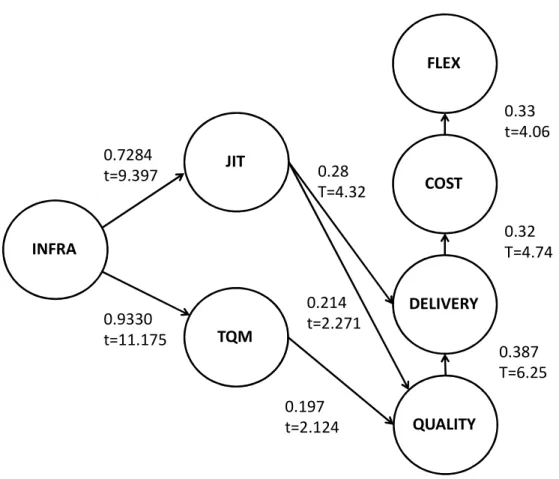
To test whether the sand cone model sequence of cumulative capabilities could be generalizable and better than the others possible sequence, I test also a rival model, following the most frequently cited rival sequence of the sand cone model, in which quality conformance and delivery are positioned in the same way, while cost and flexibility are opposite related to the sand cone model (delivery improves cost and cost improves flexibility). The results of the rival model are reported in figure 2.3. Even though also in this case the sequence of operational performances is statistically supported, it is possible to compare the models through a evaluation of Model AIC and Model CAIC.
The sand cone model has a Model AIC = 813.51 and a Model CAIC = 1070.49; while the rival model has a Model AIC = 865.13 and a Model CAIC = 1122.11. Since the sand cone model has both model AIC and model CAIC values lower than the rival model, I can assert that the sand cone model describes the best sequence of operational performance.
Moreover, fit indices of the rival model are not acceptable, indeed χ² = 754.92; d.f. = 246; χ²/d.f. = 3.07 that is higher than the cutoff value of 3; RMSEA = 0.081, higher than 0.08; CFI = .94, lower than .95.
32 INFRA JIT TQM COST FLEX DELIVERY QUALITY 0.7284 t=9.397 0.9330 t=11.175 0.309 T=4.557 0.214 t=2.271 0.197 t=2.124 0.387 t=5.93 0.669 t=7.255 0.336 t=4.732
33 INFRA JIT TQM FLEX COST DELIVERY QUALITY 0.7284 t=9.397 0.9330 t=11.175 0.28 T=4.32 0.214 t=2.271 0.197 t=2.124 0.387 T=6.25 0.32 T=4.74 0.33 t=4.06
Figure 2.3: structural model results of the rival model
Table 2.5: standardized indirect effects coefficients (t-test value)
Quality Delivery Flexibility Cost Infrastructure .57 (5.7) .52 (6.3) .28 (5.1) .14 (3.8) Total Quality Management - .12 (2.1) .10 (2.0) .09 (1.97) Just In Time - - .30 (4.5) .15 (3.5) Quality - - .19 (4.9) .09 (3.7) Delivery - - - .26 (4.5)
34
2.4
Discussion
The results found provide several implications for theory and practice. This research combines in a broad theoretical framework all LM practices (manufacturing capabilities), how they are grouped in bundles, how they are connected and their impact on operational performance (competitive capabilities). The results confirm that the implementation of all LM practices lead to an overall improvement of operational performances (Shah and Ward, 2003; Shah and Ward, 2007).
However, this research deeply analyses the mechanism by which LM builds a sustainable competitive advantage. Unlike previous empirical studies that measured LM with non comprehensive scales (e.g. Li et al., 2005), or that conclude that LM practices are not clearly causal related (e.g. Shah and Ward, 2007), I further investigated possible LM practices relationships, measuring LM with comprehensive scales and dividing them in three main bundles: Infrastructure, JIT and TQM.
Structural equation results suggest that the Infrastructure acts as an antecedent of JIT and TQM. This means that, when implementing LM, to facilitate at the later stage the implementation of JIT and TQM, managers have to consider as a priority the introduction of HRM practices to prepare the right environment for LM technical tools (Furlan et al., 2011), following a continuous improvement based strategy commonly accepted by the managers of the organization and its key suppliers (Flynn et al., 1995; Swink et al., 2005) and introducing TPM techniques (Cua et al., 2001; McKone et al., 2001).
I decided to adopt the perspective of the “sand cone” model as reference to understand the right sequence of technical bundles adoption, thus to link LM capabilities with competitive capabilities. Ferdows and De Meyer (1990) suggests to build competitive capabilities in sequence and cumulative.
The authors proposes to fix as first objective of a company a improvement of quality capability. When the first objective is sufficiently achieved, the second step of the “sand cone” model sustains to continue to improve quality and at the same time start to improve delivery capability, after that quality, delivery and flexibility, and finally quality, delivery, flexibility and cost all together. In this way manufacturers are able to
35
overcome the trade-off problem, since they don’t have to concentrate on a competitive capability at the expense of another one.
Based on this model, I connected the four dimensions of operational performances and I linked the LM part (manufacturing capabilities) with the operational performances (competitive capabilities). Structural model results demonstrate that the TQM bundle directly improve quality performance that represents the baseline of the competitive capabilities, while the JIT bundle directly improve quality and delivery capabilities.
These results are in line with LM research stream. TQM practices (Statistical Process Control, Process Feedback, Top-Management Leadership for Quality, Customer Involvement and Supplier Quality Involvement) reduce scraps and reworks, resulting in a reduction of process variability and a improvement of quality conformance of the final product (Flynn et al., 1995; Shah and Ward, 2003). JIT practices (Daily Schedule Adherence, Flow Oriented Layout, JIT links with suppliers, Kanban and Setup Time Reduction) reduce lead times, having a direct impact on delivery performance, but also directly improve quality conformance because JIT practices decrease process variability. As a matter of fact, JIT decreases the possibility to produce defects because it reduces the number of production process activities, eliminating errors associated to these activities eliminated (Green and Inman, 2005), and reduces lot sizes, permitting to find scraps and defects rapidly (Flynn et al., 1995).
These findings are fundamental advancements in LM theory and give important insights to managers because clearly demonstrate that LM practices have a optimal sequence of implementation, going beyond the common view based on the configural LM approach supported by Shah and Ward (2007).
If Infrastructure bundle represents the baseline of LM capabilities because antecedes JIT and TQM, the empirical results of this chapter suggest to implement TQM to improve quality conformance capability, and only at the end of the Lean transaction, JIT practices could be introduced to foster the impact on quality and start to improve delivery capability.
Moreover, all three LM bundles have a indirect positive effect on the last two competitive capabilities. Thus, following the implementation sequence suggested, and continuing to leverage on all LM practices, it is possible to achieve multiple – performance excellence, following the “sand cone” model sequence.
36
Finally, this chapter demonstrates the validity of the “sand cone” model in absolute terms, verifying that the sequence of operational performances are directly and indirectly connected, and in relative terms, comparing the model with the most cited rival sequence and demonstrating that the “sand cone” model fit is statistically better.
2.5
Conclusions
LM is a complex system of interrelated socio-technical practices (Shah and Ward, 2007). From an academic point of view it is vital to capture all LM aspects when empirically measuring it with the aim at making significant theoretical contributions (McCutcheon and Meredith, 1983). This research, after an extensive literature review, operationalized LM with three main bundles composed by 17 constructs related to different practices that cover LM globally.
The most common interpretation of LM in OM literature is in a configural way, namely that the more practices are implemented in a certain configuration, the more impact on performances could be obtained. This approach is coherent with the Resource Based View Theory that asserts that combination of unique resources, capabilities and manufacturing competences guides firms to a sustainable competitive advantage since it is difficult to imitate by the competitors (Prahalad and Hamel, 1994).
From a managerial point of view, the difficulties that arise when implementing LM are connected with the typical resource shortage of a manufacturing firm (Skinner, 1969) that inhibits the introduction of the LM practices at the same time. Thus, the importance of understanding the right sequence of LM practices implementation is highly strategic since the introduction of LM must be gradual, not only for the scarcity of the resources, but also because in manufacturing companies it is usual to have cultural resistance to change, mainly due to a lack of employees and managers training and education (Crawford et al., 1988). For these two reasons, LM introduction must be gradual.