Investigation of Matching Problems using Constraint Programming and Optimisation Methods

(1)

U

NIVERSITY

C

OLLEGE

C

ORK

, I

RELAND

DISI - Department of Computer Science and Engineering

Investigation of Matching Problems

using Constraint Programming and

Optimisation Methods

Dottorato di Ricerca in

Computer Science and Engineering

Ciclo: XXXIII

Settore Concorsuale: 09/H1

Settore Scientifico Disciplinare: ING-INF/05

Presentata da:

Danuta Sorina Chisca

Coordinatore Dottorato : Professor Paolo Ciaccia

Supervisore: Professor Barry O’Sullivan (UCC)

Professor Michela Milano (UNIBO)

(2)

List of Figures

1.1 An instance of SM . . . 3

1.2 An instance of popular matching . . . 5

2.1 4-Queens problem . . . 12

2.2 Example: remote village . . . 18

2.3 Decomposition of master - subproblem . . . 19

2.4 Master problem and sub-problem . . . 22

2.5 An instance of the Hospitals/Residents problem . . . 24

2.6 An instance of the Stable Roommates problem . . . 27

2.7 An instance of preference list . . . 28

2.8 An istance of HA . . . 29

2.9 An istance of HA with no popular matching . . . 33

2.10 An instance with copies which does not admit a popular matching. . . 34

2.11 A pairwise exchange . . . 39

2.12 A 3-way chain example . . . 40

2.13 An example of KEP pool [Mak-Hau, 2015] . . . 41

2.14 Example of KEP graph [Abraham et al., 2007a]. . . 43

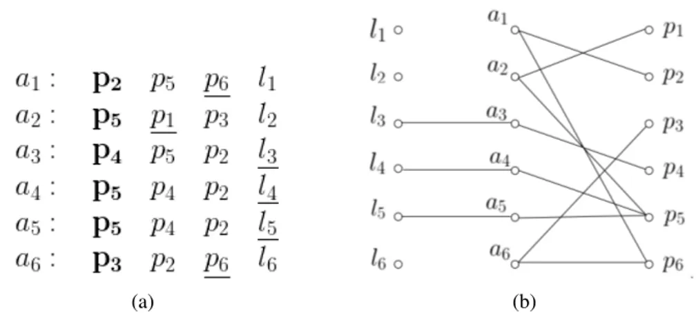
3.1 An example without ties in the preference lists (a) and the reduced graph G0 (b). . . 51

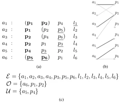
3.2 An example with ties in the preference lists and the graph G1 with a maximum matching in bold and the E , O, U labelling sets associated. 52 3.3 A perfect matching instance. . . 56

3.4 Illustration of the Flow Circulation problem. . . 57

3.5 Illustrations of the copy of a post in O in G1. . . 60

3.6 Illustration of the copy of a post in U in G1. . . 61

3.7 Illustration of the copy of a post in E in G1. . . 62

3.8 Illustration of the posts automaton. . . 63

3.9 Illustration of the applicants automaton. . . 63

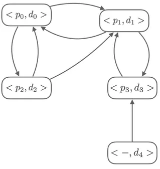
4.1 Example graph of a cycle formulation . . . 82

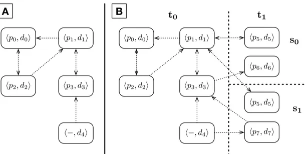
4.2 A: Example graph for an off-line KEP. B: Example graph for a scenario-based anticipatory approach . . . 84

4.3 A: A non-anticipatory solution. B: The solution returned by APST1; C: the solution with the best expected value (returned by APST2 in this case) . . . 86

4.4 A) A “concrete" compatibility graph; B) The corresponding AEG; C) The AEG-base graph used in optimization . . . 90

4.5 Trend of the algorithms for 31 months instance . . . 100

4.6 Trend of the algorithms 51 months instance . . . 101

4.7 Comparison of #transplants and #waiting list of the algorithms 15 batch setup. . . 108

4.8 Comparison of #transplants and #waiting list of the algorithms 20 batch setup. . . 108

(6)

4.10 Trend of the algorithms batch 20 setup. . . 110

4.11 Times of the algorithms . . . 110

5.1 Resolution time with b=1 log scale . . . 132

5.2 Number of master’s iterations with b=1 log scale . . . 133

5.3 Illustration of a kidney exchange rematch with 16 pairs. . . 135

5.4 Illustration of a kidney exchange rematch with 16 pairs and 1 altruistic donor. . . 135

(7)

List of Tables

3.1 Popular matching: Summary of the results . . . 68

3.2 Summary of the results for small instances . . . 70

3.3 Summary of the results for large instances . . . 71

3.4 FIXINGCOPIES: 100 applicants, 50 and 100 posts, 10% and 20% upper bound, and h = 50% . . . . 72

3.5 FIXINGCOPIES: 100 applicants, 50 and 100 posts, 10% and 20% upper bound, and h = 70% . . . . 75

3.6 FIXINGCOPIES: 200 applicants, 100 and 200 posts, 20% and 40% up-per bound, and h = 50% . . . . 76

3.7 FIXINGCOPIES: 200 applicants, 100 and 200 posts, 20% and 40% up-per bound, and h = 90% . . . . 77

4.1 31 months instance . . . 100

4.2 51 months instance . . . 101

4.3 Batch configuration 31 months instance with fix drops out . . . 102

4.4 Batch configuration for 51 months instance . . . 102

4.5 31-months setup sample algorithms (batch 5) . . . 104

4.6 31-months setup AEG (batch 5) . . . 105

5.1 Solutions of the Reformulation and Benders decomposition . . . 131

5.2 Solutions of Benders decomposition . . . 131

5.3 Summary of instances using the cycle formulation model. . . 133

(8)

nology, Cork, Ireland and Alma Mater Studiorum - Università di Bologna, Computer Science and Engineering (DISI) department, Bologna, Italy. Parts of this work have appeared in the following publications which have been subject to peer review:

• Danuta Sorina Chisca, Mohamed Siala, Gilles Simonin, and Barry O’Sullivan.

A CP-based approach for popular matching". Published in the Thirtieth

AAAI Conference on Artificial Intelligence, Phoenix, Arizona, USA, pages 4202–4203, 2016. ISBN 978-1-57735-760-5 [Chisca et al., 2016]

• Danuta Sorina Chisca, Mohamed Siala, Gilles Simonin and Barry O’Sullivan.

New Models for Two Variants of Popular Matching. Published in: 2017

IEEE 29th International Conference on Tools with Artificial Intelligence (IC-TAI), Boston, USA, pages 752–759, 2017. DOI: 10.1109/ICTAI.2017.00119 [Chisca et al., 2017]

• Danuta Sorina Chisca, Michele Lombardi, Michela Milano and Barry

O’Sullivan. From Offline to Online Kidney Exchange Optimization.

Pub-lished in: 2018 IEEE 30th International Conference on Tools with Artifi-cial Intelligence (ICTAI), Volos, Greece, pages 587–591. DOI: 10.1109/IC-TAI.2018.00095 [Chisca et al., 2018]

• Danuta Sorina Chisca, Michele Lombardi, Michela Milano and Barry

O’Sullivan. A Sampling-free Anticipatory Algorithm for the Kidney

Ex-change Problem. In Proceedings of the 16th International Conference on

the Integration of Constraint Programming, Artificial Intelligence, and Oper-ations Research, CPAIOR 2019, Thessaloniki, Greece, pages 146–162, 2019. [Chisca et al., 2019b]

• Danuta Sorina Chisca, Michele Lombardi, Michela Milano and Barry O’Sullivan. Logic-Based Benders Decomposition for Super Solutions: an Ap-plication to the Kidney Exchange Problem. In Proceedings of 25th International Conference on Principles and Practice of Constraint Programming, CP 2019, Stamford, USA, pages 108–125, 2019. [Chisca et al., 2019a]

This research was undertaken at the Insight Centre for Data Analytics and supported by Science Foundation Ireland under Grant Number SFI/12/RC/2289, which is co-funded under the European Regional Development Fund.

(9)

Acronyms

AEG - Abstract Exchange Graph

CHA - Capacitated House Allocation problem CP - Constraint Programming

CSBA - Collective Scenario-Based Algorithm CSP - Constraint Satisfaction Problem

gcc - global cardinality constraint HA - House Allocation

HAT - House Allocation with Ties HR - Hospitals/Residents Problem KEP - Kidney Exchange Problem

LBBD - Logic-Based Benders Decomposition MP - Master Problem

SP - Sub Problem

SM - Stable Marriage Problem SR - Stable Roommates problem

(10)

(11)

Acknowledgements

“It’s not that I’m so smart, it’s just that I stay with problems longer.” Einstein

There are many people that have helped me with doing this thesis and to whom I owe a debt of gratitude. Firstly, I would like to thank immensely my both supervisors, Barry O’Sullivan and Michela Milano, for their constant support and guidance; without their vision and expertise this thesis would certainly not be what it is today.

I’m very grateful to be able to work with the “popular” postdocs Gilles Simonin and Mohamed Siala, for their help in my search of “popularity”. Collaborating with them allowed me to acknowledge theoretical algorithms, which I was unaware at the mo-ment. Huge thanks to Michele Lombardi for his dedication to seek/try different algo-rithms and his continuous sustain over the years. I gained much from Michele knowl-edge, insight and enthusiasm.

I’ve been fortunate to share great times, delicious food, and in-depth conversations with many friends. In Bologna I had the pleasure to share the desk and to maintain a close friendships with Allegra, you have been a constant source of everything from deep life advice to drinking, spritz and orange juice. I’m also grateful to my “Insight” supporters: to Chrys - you always pushed me to do better, spinning and drinking coffee; to Samreen - so grateful for all the dinners we had when visiting you, P.S.: you make the most amazing biryani; to Caitríona - your patience was enormous for “rompipalle” me when asking you to remind me if I have all the documents and always forgetting one or two. It was a pleasure to share the apartment with Sarah and Aida, and so many thanks to my ex-housemates for “wining” together at the end of the day. Even if we don’t live together Sarah you are still the best runner at 5 am, and Aida you definitely know how to shake it off at the end of the day.

Lastly, and most importantly, I would like to thank my family and second family for their love, understanding, support and encouragement through all aspects of my project.

(12)

Abstract

This thesis focuses on matching under ordinal preferences, i.e. problems where agents may be required to list other agents that they find acceptable in order of preference. In particular, we focus on two main cases: the popular matching and the kidney exchange problem. These problems are important in practice and in this thesis we develop novel algorithms and techniques to solve them as combinatorial optimisation problems. The first part of the thesis focuses on one-sided matching on a bipartite graph, specifically the popular matching. When the participants express their preferences in a cardinal or-der, the most common desire is to maximise a utility function, for example finding the maximum weight or minimum cost matching. If preferences are ordinal in nature, one might want to guarantee that no two applicants are inclined to form a coalition in order to maximise their welfare, thus finding a stable matching is needed. Therefore, negoti-ating the size and the optimality of the matching with respect to agents’ preferences is a problem that occurs naturally. Popularity is a concept that offers an attractive trade-off between these two notions. In short, a popular matching is a matching in which the majority of the participants will decide on a matching M . In particular, we examine the popular matching in the context of constraint programming using global constraints. We discuss the possibility to find a popular matching even for the instances that does not admit one.

The second part of the thesis focuses on non-bipartite graphs, i.e. the kidney exchange problem, a recent innovation that matches patients in need of a kidney to willing liv-ing donors. Kidney transplant is the most effective treatment to cure end-stage renal disease, affecting one in every thousand European citizens. Chronic kidney disease is a life threatening health issue that affects millions of people worldwide. Motivated by the observation that the kidney exchange is inherently a stochastic online problem, first, we give a stochastic online method. This methos is more general and provides an expected value estimation that is correct within the limit of sampling errors. Sec-ond, we show that by taking into consideration a probabilistic model of future arrivals and drop-offs, we can get reduce sampling scenarios, and we can even construct a sampling-free probabilistic model, called the Abstract Exchange Graph (AEG). A fi-nal contribution of this thesis is related to finding robust solutions when uncertainty occurs. Uncertainty is inherent to most real world problems. For instance in the case of Kidney Exchange Problem (KEP), if a pair pools out from the solution we need to find a repair solution quickly to limit the impact to other pairs. We propose a method that exploits a Logic-Based Benders Decomposition to find super solutions to an opti-misation problem.

(13)

Abstract

L’obiettivo di questa tesi è quello di studiare problemi di matching (accoppiamento) con preferenze ordinali, i.e. problemi dove è necessario che gli agenti esprimono le loro preferenze in una lista ordinata.

La prima parte della tesi si concentra su problemi di matching unilaterale in un grafo bipartito: il popular matching. Se i partecipanti esprimono le loro preferenze in ordine cardinale, il modo più comune è di massimizzare una funzione di utilità, per esempio trovare il peso massimo oppure il costo minimo del matching. Se le preferenze sono fornite in modo ordinale, si dovrebbe garantire che nessuno dei due partecipanti creasse una coalizione in modo da massimizzare il proprio welfare, quindi trovare un matching stabile è necessario. Quindi negoziare il matching tra la dimensione e ottimalità con rispetto alle preferenze degli agenti è un problema che si verifica in modo naturale. Il concetto di popolarità (popularity) offre un compromesso di queste due nozioni. Brevemente, un matching popolare è un matching in cui la maggioranza degli agenti scelgono il matching M . In particolare, esaminiamo il matching popolare nel contesto di constraint programming (programmazione a vincoli) facendo uso dei vincoli globali. Discutiamo la possibilitá di trovare un matching popolare anche per le istanze che non ne ammettono una.

La seconda parte della tesi si concentra su un grafo non-bipartito, i.e. lo scambio dei reni - kidney exchange problem (KEP), un’innovazione recente che accoppia i pazienti bisognosi di un rene a donatori viventi disponibili. Il trapianto dei reni è il trattamento più efficace per chi soffre di un’insufficienza renale all’ultimo stadio, che colpisce una persone su mille nei paesi europei. Molto spesso un paziente bisognoso di un trapianto ha un amico o familiare che sono disposti a donare il loro rene. Tuttavia, a causa delle differenze del tipo di sangue e la presenza di certe proteine nel sangue, il donatore potenziale potrebbe risultare incompatibile con il paziente. Quindi un trapianto non può essere effettuato, oppure se si decide di procedere comunque il paziente sarebbe ad alto rischio di respingere il rene del donatore. La malattia renale cronica è un gravissima problema per la salute che colpisce milioni di persone al mondo. Motivati dall’osservazione che lo scambio dei reni è un problema online intrinsicamente sto-castica, Per primo, diamo un metodo stocastico online che è più generale e forniamo una stima del valore atteso che è corretta entro i limiti degli errori di campionamento. Secondo, facciamo vedere che prendendo in considerazione un modello probabilistico di nuovi arrivi e uscite, ci liberiamo degli scenari e possiamo costruire un modello probabilistico senza campionamento, chiamato Abstract Kidney Exchange (AEG). Un contributo finale di questa tesi e’ relativo a trovare soluzioni robuste considerando delle

(14)

incertezze. Proponiamo un metodo sfruttando la Logic Based Benders Decomposition per trovare le super soluzioni di un problema di ottimizzazione. Il master si occupa del problema originale, mentre i sottoproblemi cercano di trovare soluzioni da riparare ogni perturbanza.

(15)

Introduction

"In God we trust, all others must bring data." W. Edwards Deming

1.1 Motivation

Matching problems involving preferences are motivated in practice in widespread applications, such as the assignment of children to schools, junior doctors to hospitals, kidney transplant patients to donors and so on [Manlove et al., 2007,

Kavitha and Nasre, 2009, Irving, 2007a, Gardenfors, 1975, Biró, 2008]. Given the

applications of matching problems, and the implications of a participant’s alloca-tion in a matching for their quality of life, it is of paramount importance that the matching algorithms that drive such applications should optimise in some sense the satisfaction of the participants according to their preferences [Manlove, 2013, Gale and Shapley, 1962]. Since execution time is a very important requirement in prac-tice, a lot of the research effort has gone into developing efficient algorithms for solv-ing these matchsolv-ing problems [Hebrard et al., 2004b, Holland and O’Sullivan, 2005a, Hebrard and Walsh, 2005]. These factors have led to a lot of research activity in the area.

This thesis investigates two important variants of matching theory, and shows how Constraint Programming and Operational Research can be applied to combinatorial optimisation problems. These problems are growing in importance and we address the design, analysis and real-world applications of matching problems of indivisible goods, such as the popular matching problem and the kidney exchange problem. We focus

(16)

on the creation of new mathematical models for these problems that more accurately reflects the reality, and the development of optimal models that can be deployed in practice.

1.2 Matching Under Ordinal Preferences

Matching problems involve the assignment of a set (or sets) of agents to one another, subject to some criteria. In many cases the agents form two disjoint sets, and we seek to assign the agents in one set to those in the other.

We focus on the case where agents have ordinal preferences over a subset of the others, meaning that there is a notion of first choice, second choice, and so on. For example a student who is applying for admission to university might rank in order of preference a small list of available universities, i.e. four universities. Similarly, the universities might form a ranking of their applicants according to some academic criteria.

Matching problems with preferences can be classified into three major groups:

A. bipartite matching problems with two-sided preferences, where the agents can be partitioned into two disjoint sets, and each member of one set ranks a sub-set of the members of the other sub-set in order of preference. Example appli-cations include assigning junior doctors to hospitals [NRMP, 2019, car, 2019], pupils to schools [Abdulkadiro˘glu et al., 2005] and school- leavers to universi-ties [Biró, 2008].

B. bipartite matching problems with one-sided preferences consist of partitioning the agents into two disjoint sets, but each member of only one set ranks a subset of the members of the other set in order of preference. Example applications in-clude campus housing allocation problem [Chen and Snmez, 2002] , DVD rental markets [Abraham et al., 2006] and assigning reviewers to conference papers [Garg et al., 2010].

C. non-bipartite matching problems with preferences, where the agents form a sin-gle homogeneous set, and each agent ranks a subset of the others in order of preference. Example applications include stable roommates problem, form-ing pairs of agents for chess tournaments [Kujansuu et al., 1999], findform-ing kid-ney exchanges involving incompatible patient–donor pairs [Roth et al., 2004, Wallis et al., 2011, Dickerson et al., 2012b].

For bipartite matching problems with preferences, an extensively studied problem is the classical Stable Marriage Problem (SM)[Gale and Shapley, 1962], in which the

(17)

participants consist of two disjoint sets of agents, say n men and n women, each of whom ranks all members of the opposite sex in order of preference and a matching is just a one-one mapping between the two sets. Note that we henceforth use the term agents to refer to those participants in matching problems who have preference lists. Hence, the agents in a SM instance are the men and women.

In [Gale and Shapley, 1962] the authors showed that, given an SM instance of size n, a stable matching can always be found in polynomial-time, and moreover they also

provided an O(n2_{) algorithm to find such a matching. The algorithm involves a}

se-quence of marriage proposals made by the members of one sex to the members of the other. Each proposal is followed by either an acceptance or a rejection. Proposals are accepted if the person being proposed to is either unmatched or prefers the proposer to his/her current partner, in which case his/her current partner is rejected in favour of the new proposal. Proposals are rejected if the person being proposed to already has a partner he/she prefers to the proposer. The algorithm can be executed with the men doing the proposing (man-oriented) or with the women doing the proposing (woman-oriented). Agents of the proposing set start with the most preferred agents on their preference lists and make proposals until they are accepted. If they ever get rejected due to their partner getting a better proposal from someone else, they continue by mak-ing a proposal to the next agent on their preference list. The algorithm terminates when all parties involved are matched.

Men’s preferences: Women’s preferences:

m1 : w1, w2, w3, w4 w1 : m4, m3, m2, m1 m2 : w2, w1, w4, w3 w2 : m3, m4, m1, m2 m3 : w3, w4, w1, w2 w3 : m2, m1, m4, m3 m4 : w4, w3, w2, w1 w4 : m1, m2, m3, m4 <latexit sha1_base64="ddJ1EtSZD0uNlI4MWIfDI3mbiWs=">AAADUHicbZLPa9swFMdlZz8671e6HXcRS8Z2KMGyDS09FXbZZdDC0hTiYGRFbkUt25XkpsHkT9ylt/0du+ywscqyY7a6D/z0eO+rj57kFxcpk8p1f1j24NHjJ093njnPX7x89Xq4++ZU5qUgdEryNBdnMZY0ZRmdKqZSelYIinmc0ll8+bmuz66pkCzPvql1QRccn2csYQQrnYp2rSRU9EZVX2n2UUK9NaGCZoTKww0Mr65KvNwuEDbKWc772jB0nDGPEDyEqwjtaefVzq9d0APVGq3kUbCnnV87r3Zo3HI8wzEIAwsMrANs15URtgTDQoa1xfgG43eEprFeOysj3PbQsfwxbDmB4QTdjZrGHuAEhoO6CzWN1ZxoOHInrjHYD1AbjEBrx9HwNlzmpNRvrUiKpZwjt1CLCgvFSEo3TlhKWmByic/pXIcZ5lQuKjMQG/hBZ5YwyYX+MgVN9t8dFeZSrnmslRyrC3m/Vicfqs1LlRwsKpYVpdJ/vjkoKVOoclhPF1wyQYlK1zrARDDdKyQXWGCi9Aw6+hHQ/Sv3g1NvgvyJd+KNjtz2OXbAO/AefAII7IMj8AUcgykg1nfrp/Xb+mPf2r/svwOrkdrtCt6C/2zg3AGUIPfF</latexit> Figure 1.1: An instance of SM

For example in Figure 1.1, we have a set of 4 men and a set of 4 women, seeking for a match, and there are 10 stable matchings [Knuth, 1976]:

(18)

M1 = {(m1, w1), (m2, w2), (m3, w3), (m4, w4)}, M2 = {(m1, w2), (m2, w1), (m3, w3), (m4, w4)}, M3 = {(m1, w1), (m2, w2), (m3, w4), (m4, w3)}, M4 = {(m1, w2), (m2, w1), (m3, w4), (m4, w3)}, M5 = {(m1, w2), (m2, w4), (m3, w1), (m4, w3)}, M6 = {(m1, w3), (m2, w1), (m3, w4), (m4, w2)}, M7 = {(m1, w3), (m2, w4), (m3, w1), (m4, w2)}, M8 = {(m1, w3), (m2, w4), (m3, w2), (m4, w1)}, M9 = {(m1, w4), (m2, w3), (m3, w1), (m4, w2)}, M10= {(m1, w4), (m2, w3), (m3, w2), (m4, w1)}.

Alternatively to SM, preference lists for bipartite matching problems can be one-sided. An example of this type of problem is the House Allocation problem (HA) [Abraham et al., 2004], where an attempt is made to allocate a set H of objects (e.g., houses, posts etc) using a one-one mapping among a set A of agents, each of whom ranks a subset of H in order of preference.

In addition to bipartite matching problems, non-bipartite matching problems

are also widely studied. In the classical Stable Roommates problem (SR)

[Gale and Shapley, 1962, Irving, 1985], the participants consist of a single set of agents each of whom ranks the others in order of preference, and a matching is a partition of the set into disjoint pairs of roommates.

1.3 The Popular Matching Problem

In the one sided bipartite graph, each applicant has an ordinal preference list, ranking the subset of items in order of his preference (first choice, second choice, and so on). We seek to match applicants to items in which no applicant is matched with more than one item, and no item is matched with more than one applicant. We will consider that the preference lists are not strictly ordered, for example an applicant might have two items as first choice in his preference list (a tie).

Consider the example below with three applicants and three items, and the respective preference list:

(19)

Figure 1.2: An instance of popular matching

Let M and M0 be two arbitrary matchings in a given instance I and let P(M,M0) denote

the set of agents who prefer M to M0. We say that M is more popular than M0 if

|P (M, M0_{)| > |P (M}0_{, M )|, i.e. the number of agents who prefer M to M}0 _{is greater}

than the number of agents who prefer M0 to M. A matching M in I is popular if there

is no other matching M’ in I that is more popular than M [Abraham et al., 2007a]. In Figure 1.2, consider the three symmetrical matchings:

M1 = {(a1, p1), (a2, p2), (a3, p3)} M2 = {(a1, p3), (a2, p1), (a3, p2)} M3 = {(a1, p2), (a2, p3), (a3, p1)}

It is easy to verify that none of these matchings is popular, since M1 < M2, M2 < M3,

and M3 < M1. In fact, this instance admits no popular matching, the problem being

that the more popular than relation is not acyclic. The popular matching problem is to determine if a given instance admits a popular matching and to find such a matching, if one exists.

Gardenfors [Gardenfors, 1975] first introduced the notion of a popular matching, the author referres to this concept as a majority assignment in the context of vot-ing theory. We remark that the more popular concept can be traced back even fur-ther to the Condorcet voting protocol. Popular matchings were then considered by [Sng and Manlove, 2010] in the context of the House Allocation (HA) problem. They showed that popular matchings need not exist, given an instance of HA, and also noted that popular matchings can have different cardinalities. In [Abraham et al., 2007a] au-thors described an O(n + m) algorithm for finding a maximum cardinality popular matching (henceforth a maximum popular matching) if one exists, given an instance

of HA. They also described an O(√nm) counterpart for the House Allocation with

ties (HAT) problem.

There exist in the literature a number of efficient algorithms for solving popular match-ing problems, e.g. [Abraham et al., 2007b]. In [Huang and Kavitha, 2013, Biró, 2008] the authors design the popular matching for the stable marriage problem and the room-mates problem. In [Acharyya et al., 2014] they count the number of popular matchings

(20)

in the House Allocation Problem. In [Mestre, 2006] the author studied the weighted version of popular matching problem. However, in real world situations, additional constraints are often needed. In many cases, the new problem is intractable and the original algorithms become useless.

1.4 Kidney Exchange Problem

The Kidney exchange is a recent innovation that matches patients in need of a kidney to willing donors. In a non-bipartite graph, we can model the kidney exchange problem by constructing a pair (patient, donor) for each patient, and an directed edge between any two pairs where the incompatible donor for one patient is compatible with the

other patient, and viceversa. An edge (pi,pj) in a matching corresponds to a pairwise

kidney exchange, in which pj receives a kidney from pi’s donor in exchange for pi

receiving a kidney from pj’s donor. Preference lists can be constructed on the basis of compatibility profiles between donors and patients.

For example, (Mary and Carlos) and (Amir and Shauna) are two incompatible pairs, where Mary wants to donate a kidney to Carlos, but they do not match; Amir wants to donate to Shauna, but they do not match. Mary is a match for Shauna, and Amir matches Carlos. Swapping donors and patients in this case allows both transplants to happen. An exchange cycle (or simply “cycle”) involves a sequence of matches where the donor of one pair donates to the candidate in the next pair along the cycle. The cycle is completed when the donor in the last pair gives a kidney to the candidate in the first pair [Roth et al., 2005]. An "altruistic" donor can initiate chains of transplants in the pool that end by transplanting a candidate on the deceased donor waiting list, called domino-paired donation (DPD) [Roth, 2008].

Traditionally, a KEP pool is managed through a sequence of match runs, whereby at regular intervals, the pool is assessed and a solution consisting of cycles and chains is determined such that no pair is simultaneously involved in more than one cycle or chain. In larger pools, there are many cycles and/or chains and consequently many possible solutions. The preferred selection would ideally be determined by some objective function, such as maximising the total number of potential transplants [Roth et al., 2004]. In cycles there is a practical limitation that all transplants should be performed simultaneously in order to avoid the possibility of a scheduled donor opting to leave the pool prior to donation. Without this restriction, the possibility ex-ists that a donor will donate a kidney without the associated candidate obtaining a transplant. For this reason, if any one of the transplants in a proposed cycle cannot

(21)

be completed, none of the selected transplants in the cycle can proceed. On the other hand, if one of the transplants in a proposed chain segment cannot be completed, trans-plants prior to the point of failure can still proceed since the issue of an untransplanted candidate with no donor does not arise [Ashlagi et al., 2011, Anderson et al., 2015]. Failure to proceed with a proposed solution can occur for a number of reasons, includ-ing a positive laboratory crossmatch, a candidate or physician declininclud-ing an assigned donor, or donors or candidates having to leave the pool due to illness or other reasons [Dickerson et al., 2013].

Recent studies suggest that optimisation methods which take into account the prob-ability that selected transplants fail to proceed to actual transplantation can improve upon schemes that ignore this uncertainty [Dickerson et al., 2013, Alvelos et al., 2015, Pedroso, 2014]. However, these programs run offline, at prefixed intervals, we ar-gue that the problem is intrinsically a dynamic problem which evolves in time. In [Ünver, 2010] he provides initial analysis on dynamic kidney exchange, but does not include chains in the program. In [Pedroso, 2014] they develop a dynamic scheme, considering even the case of compatible pairs, however the program still runs at fixed terms. In [Dickerson and Sandholm, 2015] the authors build a future match frame-work, learning the potentials of pairs in an offline graph.

1.5 Contribution and Thesis Structure

In this section, we discuss the structure of this thesis, along with the contributions of each chapter and the overall contributions of the methods presented in the thesis.

Background

Chapter 2 begins by presenting an introduction to the field of optimisation in combina-torial problems. We give a brief overview of several important results from matching theory; some of these will subsequently be used by the algorithms that we will de-scribe in this thesis. Instances of constraint programming, integer programming and Logical-based Benders Decomposition are shown as high level encoding.

Background

“I have been impressed with the urgency of doing. Knowing is not enough; we must apply. Being willing is not enough; we must do.” Leonardo da Vinci

In this chapter we provide the necessary background to understand the matching prob-lems. Moreover, we will focus on optimisation problems, popular matchings, and kidney exchanges. For each of them we introduce the necessary background.

2.1 Optimisation

Numerous industrial applications of combinatorial optimisation require going beyond a single satisfiable solution. Frequently the interest is in finding good, or the absolute best, quality solution. For example, we might wish to define the objective function to maximise profit, produce customer satisfaction, or to minimise cost, loss function. Due to the potential size of the applications in practice, it is usually infeasible to com-pute optimal allocations by hand. Centralised matching schemes automate this task by employing algorithms to compute optimal matchings based on the input data supplied by the participants.

A combinatorial optimisation model of a problem consists of a declarative specifi-cation, separating the problem in the formulation and the search strategy. However, modelling a problem is difficult as a solvable model is needed to quickly finds optimal solutions or determines that none exist. Naturally, there are many alternative models for a single problem; often it is not clear which one is best. In an optimisation setting,

(25)

an objective function needs to be specified and optimised, i.e. maximise or minimise an utility function. Once the model is defined it can be passed off to a solver which will search for an optimal solution. Often, we may need to specify some heuristics about how the solver should perform the search, such as the variable or value ordering before the solver can effectively solve the problem.

Two common issues arise in the development of a solution: the model either does not accurately represent the problem, or a solution is not found by the solver in reasonable time. The former is more of a real-world problem requiring the assistance of a domain expert, while latter may require the input of an expert in combinatorial optimisation.

2.1.1 Constraint Programming

The field of constraint programming (CP) is rapidly progressing. Constraint pro-gramming [Rossi et al., 2006] is a powerful paradigm for solving combinatorial search problems using a wide range of techniques from artificial intelligence, computer sci-ence, and operations research. Constraint programming is currently applied with suc-cess to many domains, such as scheduling, planning, vehicle routing, etc. The basic idea in constraint programming is that the user states the constraints and a general purpose constraint solver is used to solve them. Constraints are just relations, and a constraint satisfaction problem (CSP) states which relations should hold among the given decision variables. For example, in scheduling activities in a company, the de-cision variables might be the starting times and the duration of the activities and the resources needed to perform them, and the constraints might be on the availability of the resources and on their use for a limited number of activities at a time. Constraint solvers take a real-world problem like this, represented in terms of decision variables and constraints, and find an assignment to all the variables that satisfies the constraints.

The constraint satisfaction problem (CSP) [Rossi et al., 2006] is defined by a tuple hX, D, Ci, defining the variables, domains, and constraints respectively. A solution to a CSP consists of a mapping from each variable in X to one of the values in its domain, such that all constraints in C are satisfied. A CP solver works by systematically trying all possible assignments of values to the variables in a problem, to find the feasible solutions.

Example: the 4-Queens Problem1 _{consists in placing four queens on a 4 × 4}

chess-board, see Figure 2.1 such that no two queens are attacking each other.

There are two key elements to a constraint programming search:

(26)

• Propagation — Each time the solver assigns a value to a variable, the constraints add restrictions on the possible values of the unassigned variables. For example, in the 4-queens problem, each time the solver places a queen, it can’t place any other queens on the row and diagonals the current queen is on. Propagation can speed up the search significantly by reducing the set of variable values the solver must explore.

• Backtracking occurs when either the solver can’t assign a value to the next vari-able, due to the constraints, or it finds a solution, therefore the solver backtracks to a previous stage and changes the value of the variable at that stage to a value that hasn’t already been tried. In the 4-queens example, this means moving a queen to a new square on the current column.

For instance, to model the 4-Queens Problem, we can create four variables queens, each of them with domain D = {1, 2, 3, 4}. For any solution, queens[i] = j means there is a queen in column i and row j.

Figure 2.1: 4-Queens problem

These constraints guarantee the three conditions for the 4-queens problem:

• no two queens on the same row

• no two queens on the same column

• no two queens on the same diagonal

These constraints can be added efficiently to the CP model. The 4-Queens problem can be extended to N-queens, but the number of solutions goes up roughly exponentially with the size of the board.

2.1.1.1 Global Constraints

Global constraints define constraints over an arbitrarily sized set of variables, present-ing many benefits for constraint programmpresent-ing [van Hoeve and Katriel, 2006]. Notably,

(27)

they can convey complex relationships between variables, allowing for a concise spec-ification of a problem. More importantly, from a pragmatic perspective, this enables higher levels of reasoning to be performed by dedicated inference algorithms, reducing the search space significantly. For example, propagation for global constraints such as

AllDifferentand cardinality constraints can be achieved in low polynomial time using

flow-based algorithms [Régin, 1994].

The Global Constraint Catalogue [Beldiceanu et al., 2007] collects definitions for all global constraints defined in the CP literature. Such a vast catalogue provided many opportunities for the application of constraint programming, however one practical issue faced by users is in identifying which one is appropriate for their problem.

All-Different

One of the most widely known, intuitive, and well studied global constraints is the AllDifferent constraint [Régin, 1994] which simply specifies that a set of variables must be assigned distinct values. Such a relation arises in many practical applications such as resource allocation, e.g. to state that a resource may not be used more than once at a single time point.

The model for the example in Figure 2.1 can can use a global constraint such as

AllD-ifferent to efficiently solve the problem. One solution of 4-Queens is shown in

Fig-ure 2.1.

Global Cardinality

The global cardinality constraint [Régin, 1996] places lower and upper bounds on the number of occurrences of certain values amongst a set of variables. The global cardinality constraint gcc(x1, . . . , xn, cv1, . . . , cvn0) is a generalization of AllDifferent.

While AllDifferent requires that every value is assigned to at most one variable, the gcc is specified on n assignment variables x1, . . . , xn and n0 count variables cv1, . . . , cvn0

and specifies that each value vi is assigned to exactly cvi assignment variables.

AllD-ifferent, then, is the special case of gcc in which the domain of each count variable

is {0, 1}. For any tuple t ∈ Dn and value v ∈ D, let occ(v, t) be the number of

occurrences of v in t.

The global cardinality constraint models restrictions in applications such as timetabling when there may be a limit on the number of consecutive activity types. An exam-ple of a problem that can be modeled with a gcc is the shift assignment problem

(28)

[Régin, 1994, van Hoeve and Katriel, 2006] in which we are given a set of workers

W = {W1, . . . , Ws} and a set of shifts S = {S1, . . . , St} and the problem is to assign each worker to one of the shifts while fulfilling the constraints posed by the workers

and the boss: Each worker Wispecifies in which of the shifts she/he is willing to work

and for each shift Si the boss specifies a lower and upper bound on the number of

workers that should be assigned to this shift. In the gcc, the workers would be repre-sented by the assignment variables and the shifts by the count variables. The domain of an assignment variable would contain the set of shifts that the respective worker is willing to work in and the interval corresponding to each count variable would match the lower and upper bounds specified by the boss for this shift.

2.1.2 Integer Programming

An integer programming problem is a mathematical optimisation or feasibility prob-lem, in which some or all the variables are restricted to be integers. Example of an optimisation problem: max n X j=1 cjxj (2.1) subject to: n X j=1 aijxj = bi ∀i ∈ m (2.2) xj ≥ 0 ∀j ∈ n (2.3)

xj integer for some or all j ∈ n (2.4)

This problem is called the linear integer-programming problem. It is said to be a mixed

integer program when some, but not all, variables are restricted to be integer, and is

called a pure integer programming when all decision variables must be integers. The case where the integer variables are restricted to be 0 or 1 comes up surprising often. Such problems are called pure (mixed) 0-1 programming problems or pure (mixed) binary integer programming problems.

Integer-programming models arise in practically every area of application of mathe-matical programming. One particularly simple integer problem is the Knapsack prob-lem [Martello and Toth, 1990]. The traditional story is that there is a knapsack, (with

capacity w0), there are a number of items, each with a weight (w) and a value (c). The

(29)

written as: max n X j=1 cjxj (2.5) s.t. n X j=1 wjxj ≤ w0 (2.6) xj ∈ {0, 1}∀j ∈ n (2.7)

Assume for example we have a knapsack (with capacity 14), and 4 items, i.e. e item 2 has weight 7 and value 11: A practical example is

max8x1+ 11x2+ 6x3 + 4x4 (2.8)

s.t.5x1+ 7x2+ 4x3+ 3x4 ≤ 14 (2.9)

xj ∈ {0, 1} (2.10)

The solution x1 = 1, x2 = 1, x3 = 0.5, x4 = 0, with value 22 is the optimal solution

to the linear program, even though is not integral. An integer solution is a x1 = 0,

x2 = 1, x3 = 1, x4 = 1 with a value of 21.

2.1.3 Super Solutions

When dealing with real world problems, efficiency and optimality may not be the only concerns. For instance, in the kidney exchange problem further tests are performed just hours before the surgery, and this may affect the solution found, i.e. the patient/donor worsening. The problem is to find a matching for the kidney exchange problem re-silient to small perturbation. The notion of fault tolerance has been introduced in the propositional satisfiability framework by [Ginsberg et al., 1998]. A solution is fault tolerant if a small change in the model is guaranteed not to result in a large perturba-tion of the soluperturba-tion.

However, one might want the new solution to be as close as possible to the old solu-tion. Indeed it might not be practical to change too many surgeries on short notice. A solution where a small perturbation, such as a pair pooling out from the solution, can be repaired with small changes. The notion of super-models [Ginsberg et al., 1998] or

(30)

"To model this concept of fault tolerance we introduce the notion of σ-models: these are satisfying assignments of Boolean formula for which any small alteration, such as a single bit flip, can be repaired by another small alteration, yielding a nearby satisfying assignment."

An (a, b) super model α is a model of a Boolean formula such that for any set of atoms A, if |A| ≤ a, then there exists a disjoint set B such that |B| ≤ b and if we negate

α(A ∪ B) we obtain another model. Below is the definition of (1, 1) super models

from [Roy, 2001, Roy, 2006]:

Definition 2.1. A super-model of a Boolean formula F is a satisfying assignment α of F, F (α) = 1, such that for every i, if we negate the i-th bit of α, there is another bit j 6= i of α which we can negate to get another satisfying assignment.

Flipping a bit of a σ-model is called a break, corresponding to a “bad” event. The bit that is flipped to get another satisfying assignment is a repair.

In [Roy, 2006] the author extended the notion of single repairability to repairability of a sequence of breaks to a model.

Definition 2.2. A σ(r, s)-model of a Boolean formula Θ is a model of Θ such that for every choice of at mostr bit flips (the “break” set) of the model, there is a disjoint set

of at mosts bits (the “repair” set) that can be flipped to obtain another model of Θ.

[Hebrard et al., 2004b] generalise this definition to constraint satisfaction on non-Boolean domains.

Definition 2.3. A solution to a CSP is (a, b)-super solution iff the loss of the values of

at mosta variables can be repaired by assigning other values to these variables, and

(31)

Let us consider the following CSP example from [Hebrard et al., 2004b]: X, Y, Z ∈ {1, 2, 3}, X ≤ Y ∧ Y ≤ Z. The solutions to this CSP are:

<1, 1, 1>, <1, 1, 2>, <1, 1, 3>, <1, 2, 2>, <1, 2, 3>, <1, 3, 3>, <2, 2, 2>, <2, 2, 3>, <2, 3, 3>, <3, 3, 3>.

The subsets of the solutions that are (1, 1)-super solutions are:

<1,1,2>, <1,1,3>, <1,2,2>, <1,2,3>, <1,3,3>, <2,2,2>, <2,2,3>, <2,3,3>

and (1, 0)-super solutions are:

<1, 2, 3>, <1, 2, 2>, <2, 2, 3>.

The solution <1,1,1> is not a (1,0)-super solution. If X loses the value 1, there is no repair value for X that is consistent with Y and Z since neither <2, 1, 1> nor <3, 1, 1> are solutions. Also, solution <1, 1, 1> is not a (1, 1)- super solution since when X loses the value 1, there is no repair by changing the value assigned to at most one other variable, i.e., there exists no repair solution when X breaks since none of <2,1,1>, <3,1,1>, <2,2,1>, <2,3,1>, <2,1,2>,<2, 1, 3> is a solution. On the other hand, <1, 2, 3> is a (1, 0)-super solution given that when X breaks the repair solution is <2, 2, 3>, when Y breaks the repair solution is <1, 1, 3>, and when Z breaks the repair solution is <1, 2, 2>.

A number of properties follow immediately from the definition. For example, a (c, d)-super solution is a (a, b)-d)-super solution if (a ≤ c or d ≤ b) and c + d ≤ a + b. Deciding if a SAT problem has an (a,b)-supermodel is NP-complete [Ginsberg et al., 1998]. In [Hebrard et al., 2004b] the authors shows that deciding if a CSP has an (a,b)-super solution is also NP-complete, even when restricted to binary constraints:

Theorem 2.1. Deciding if a CSP has an (a, b)-super solution is NP-complete for any fixeda.

Furthermore they proposed a method to find (1, 0)-Super Solutions via Search. There-fore, by choosing a (1,0)-super-solution over other solutions, we deal with one pertur-bation without changing other assignments, which is often a valuable property.

In [Holland and O’Sullivan, 2004] the authors proposed a novel application of super solutions to combinatorial auctions in which a bid may be disqualified or withdrawn after the winners are announced. In [Holland and O’Sullivan, 2005b] they proposed a Weighted Super Solutions to find a repair solution whose revenue exceeds some threshold while limiting the cost associated with forming such a repair.

(32)

A more recent paper on fault tolerant solutions [Bofill et al., 2013] using SAT encod-ing, improves the work of [Ginsberg et al., 1998] using weighted Partial MaxSAT

for-mulation. Their approach strengthens the complexity to O(na) for each handled

vari-able change, where n is the number of varivari-ables, and a is the number of breaks, instead

of O(na+b) of [Ginsberg et al., 1998], where b is the number of repairs.

2.1.4 Logic-based Benders Decomposition

The Logic-based Benders Decomposition (LBBD) approach has been used so solve allocation and scheduling problems [Hooker and Ottosson, 2003, Hooker, 2007] and resource allocation [Benini et al., 2011]. LBBD is a classic operational research tech-nique, which assigns some of the variables trial values and finds the best solution con-sistent with these values. In the process it learns informations to reduce the number of solutions. This strategy is known as “learning from one’s mistakes”, as exclude su-perfluous solutions. The central element of Benders decomposition is the derivation of Benders cuts that exclude superfluous solutions. Classical Benders cuts are formulated by solving the dual of the subproblem that remains when the trial values are fixed. The subproblem must therefore be one for which dual multiplers are defined, such as a linear or nonlinear programming problem.

Fixing some primary variables to these values, solves a subproblem for each set of values. The solution of the subproblem is used to generate a cut, i.e. Bender’s cut, that the primary variables must satisfy in all solutions enumerated.

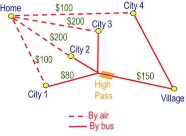
Figure 2.2: Example: remote village

(33)

village with the values shown in Figure 2.2, the village can be reached by bus or air. Let be x flight destination and y the bus route, we seek to find cheapest route (x,y). The master problem solve the cheapest flight x, subject to Benders cuts generated so far, while the subproblem search to find the cheapest bus route from the airport to the village. The master problem and the subproblem interactions as in Figure 2.3.

Figure 2.3: Decomposition of master - subproblem

We start with x = City 1 and pose the subproblem: find the cheapest route given that x = City 1. Optimal cost is $100 + 80 + 150 = $330.

The dual problem of finding the optimal route is to prove optimality. The proof is that the route from City 1 to the village must go through High Pass. So cost ≥ airfare + bus from city to High Pass + $150. But this same argument applies to City 1, 2 or 3. Specifically the Benders cut is:

cost ≥ Bcity1(x) =          $100 + 80 + 150 if x = City 1 $200 + 150 if x = City 2,3 $100 if x = City 4         

Now we need to solve the master problem, thus we need to pick the city x to minimize cost.

Clearly the solution is x = City 4, with cost $100. Now let x = City 4 and pose the subproblem: Find the cheapest route given that x = City 4. Optimal cost is $100 + 250 = $350.

(34)

cost ≥ Bcity4(x) =    $350 if x = City 1 $0 otherwise   

The solution is x = City 1, with cost $330. Because this is equal to the value of a previous subproblem, we are done.

Classical Benders cuts are formulated by solving the dual of the subproblem, when some values are fixed. Formally a general optimization problem can be written as:

min f (x) OP (2.11)

s.t. (2.12)

x ∈ S (2.13)

x ∈ D (2.14)

where f (x) is a generic function, each variable with domain D and a set of constraints

S ⊆ D.

Assume P and Q to be two propositions whose truth or false is a function of x. Then P implies Q with respect to D if Q is true for any x ∈ D for which P is true, and can be written as P−→ Q.D

The inference dual of OP0can be written as:

max β ID (2.15)

s.t. (2.16)

x ∈ S−→ f (x) ≥ βD (2.17)

The dual problem finds the tightest possible bound on the objective function value.

The optimal value of the inference dual is the same as the original problem, given the strong duality property.

(35)

LBBD Structure

Benders decomposition views elements of the feasible set as pairs (x, y) of objects that

belong respectively to domains Dx, Dy .

Therefore the optimisation problem OP0 becomes:

min f (x, y) OP (2.18)

s.t. (2.19)

(x, y) ∈ S (2.20)

x ∈ Dx, y ∈ Dy (2.21)

A general LBBD algorithm begins by fixing the variables y to some values ¯y ∈ Dy

in the master problem (MP), see Figure 2.4. This leads to the following subproblem, (SP):

min f (x, ¯y) SP (2.22)

s.t. (2.23)

(x, ¯y) ∈ S (2.24)

x ∈ Dx (2.25)

Rather than solving the subproblem directly, we can solve the corresponding inference dual, known to have the same optimal value.

max β DP (2.26)

s.t. (2.27)

(x, ¯y) ∈ S Dx

(36)

The dual problem is to find the best possible lower bound β∗ on the optimal cost that

can be inferred from the constraints, assuming y is fixed to ¯y. The optimal solution of

subproblem is the same as the tightest bound on f (x, y) for any fixed value of y, due to strong duality, which can be inferred from the constraint.

Just how this is done varies from one context to another, but essentially the idea is

this. Let β∗ be the value obtained for DP, which means that β∗ is a lower bound on

the optimal value of OP, given that y = ¯y. The solution of OP is a proof of this fact.

This bound is expressed as a function βyy¯ of y, producing a Benders cut z ≥ βyy¯ . The

subscript ¯y of the bounding function denotes the y values used for its construction.

The algorithm proceeds as follows. At each iteration the Benders cuts so far generated comprise the constraints of a master problem,

min z M P (2.29)

s.t. (2.30)

z ≥ β¯yk ∀k = 0, 1... (2.31)

y ∈ Dy (2.32)

where ¯y1, ¯y2, ... are the trial values till now obtained. The next trial value (¯z, ¯y) of (z,

y) is obtain by solving the master problem. If the optimal value β∗ of the resulting

subproblem DP is equal to ¯z. Otherwise a new Benders cut z ≥ βyy¯ is added to the

master problem. At this point the algorithm repeats. The algorithm terminates when

the master problem and subproblem value converge, that is ¯z = β∗.

(37)

In Figure 2.4 we show how the MP and SP communicates. First, the problem at hand is first decomposed into a master problem (MP) and a subproblem (SP). After the method works by iteratively solving MP and feeding SP with the partial solution from MP. If such solution cannot be extended to a complete one, a cut (Benders’ cut) is generated forcing MP to yield a different solution. In case the extension is successful we have a feasible solution. The efficiency of the technique greatly depends on the possibility to generate strong cuts.

Theorem 2.2. Suppose that in each iteration of the generic Benders algorithm, the bounding functionβy¯satisfies the following:

The Benders cut z ≥ β¯y is valid; i.e., any feasible solution (x,y) of OP satisfies

f (x, y) ≥ βy¯.

If the algorithm terminates with a finite optimal solution (z, y) = (¯z, ¯y) in the master

problem, OP has an optimal solution (x, y) = ¯x, ¯y) with value f (¯x, ¯y) = ¯z. If the

algorithm terminates with an infeasible master problem, then OP is infeasible. If the algorithm terminates with an infeasible subproblem dual, then OP is unbounded. In general, the cuts can be refined to a specific problem and needs to be valid. Because all Benders cuts are valid, infeasibility of the master problem implies that the original problem is infeasible. Finally, if the subproblem dual is infeasible, then the subproblem is unbounded, which means the original problem is unbounded.

2.2 Matching Under Ordinal Preferences

Stable matching problems, introduced by [Gale and Shapley, 1962], have been exhaus-tively studied over recent decades. Different formulations are proposed, distinguishing between one-sided matching [Garg et al., 2010] and two-sided matching, e.g. the sta-ble marriage (SM) prosta-blem [Gale and Shapley, 1962].

An instance of the classical Stable Marriage problem (SM) comprises a set of men and women, and each person ranks each member of the opposite sex in strict order of pref-erence, and we seek to match one to another taking in consideration their preferences.

A generalisation of SM is the Hospitals / Residents problem (HR) [Gale and Shapley, 1962], where each man corresponds to a resident and each woman corresponds to a hospital which can potentially be assigned multiple residents up to some fixed capacity.

The Stable Roommates problem (SR) is the non-bipartite generalisation of SM in which each agent ranks all of the others in strict order of preference. Stability is once

(38)

again relevant in this context, and the definition of a stable matching is a straightfor-ward extension of the definition in the SM case.

2.2.1 Stable Matching for Hospitals / Residents problem

The Hospitals / Residents problem (HR) [Gale and Shapley, 1962, Gusfield and Irving, 1989, Manlove, 2008] (or known as the College (or University or Stable) Admissions problem, or the Stable Assignment problem) was first defined by Gale and Shap-ley in their seminal paper “College Admissions and the Stability of Marriage” [Gale and Shapley, 1962].

An instance of HR involves a set R = {r1, ..., rn1} of residents and a set H =

{h1, ..., hn2} of hospitals. Each hospital hj ∈ H has a capacity cj, which indicates

the number of posts that hj has. Also there is a set E ⊆ R × H of acceptable

res-ident–hospital pairs. Each resident ri ∈ R has an acceptable set of hospitals A(ri),

where A(ri) = {hj ∈ H : (ri, hj) ∈ E}.

In the same way, each hospital hj ∈ H has an acceptable set of residents A(hj), where

A(hj) = {ri ∈ R : (ri, hj) ∈ E}.

Figure 2.5: An instance of the Hospitals/Residents problem

An example with six residents and three hospitals, and their respective preferences, is shown in Figure 2.5.

A matching M is an assignment such that |M (ri)| ≤ 1 for each ri ∈ R and |M (hj)| ≤

cj for each hj ∈ H, that is no resident is assigned to an unacceptable hospital, each

resident is assigned to at most one hospital, and no hospital is oversubscribed).

Definition 2.4. Let I be an instance of HR and let M be a matching in I

[Manlove, 2013]. A pair (ri, hj) ∈ E \ M blocks M , or is a blocking pair for M ,

(39)

A. riis unassigned or prefershj toM (ri);

B. hj is undersubscribed or prefersri to at least one member ofM (hj) (or both).

M is said to be stable if it admits no blocking pair. In Figure 2.5 the instance admits a

stable matching M = {(r1, h2), (r2, h1), (r3, h1), (r4, h3), (r6, h2)}.

The algorithm in [Gale and Shapley, 1962], known as the resident-oriented

Gale–Shapley algorithm (RGS), showed that every instance I of HR admits at least one stable matching.

Theorem 2.3. Given any instance of HR, the RGS algorithm constructs, in O(m) time,

the unique resident-optimal stable matching, where m is the number of acceptable

resident–hospital pairs [Gusfield and Irving, 1989, Manlove, 2013].

The RGS algorithm returns the unique resident-optimal stable matching, in which each assigned resident has the best hospital that she could achieve in any stable matching, whilst each unassigned resident is unassigned in every stable matching [Gale and Shapley, 1962].

Equivalently to the RGS algorithm, also the hospital-oriented Gale–Shapley algorithm (HGS), involves hospitals offering posts to residents. The HGS algorithm returns with

the unique hospital-optimal stable matching. In this matching, every hospital hj ∈ H

is assigned its cj best stable partners, whilst every undersubscribed hospital is assigned the same set of residents in every stable matching [Gusfield and Irving, 1989].

2.2.2 Stable Matching for Hospitals/Residents Problem with

Indif-ference

In large-scale matching schemes, participants may not be able to provide a genuine strict preference order over what may be a very large number of hospitals, and may prefer to express indifference in their preference lists, (ties). The concept of indiffer-ence can be applied to instances of HR [Manlove, 2013].

A matching in the context of Hospitals/Residents problem with indifference (HRI), is a set of (resident, hospital) pairs such that no resident is assigned to more than one hospital and no hospital is over-subscribed. A matching is stable if it admits no blocking pairs. We can define a blocking pair for an instance of HRI with respect to three different levels of stability, since the presence of ties forces us to extend the definition. In fact an hospital h can prefer ri over rj, rj over ri or to be indifferent between them, as we can see in the example below:

(40)

A pair (ri, hj) ∈ R × H is said to block a matching M for an instance of HRI, and is called a blocking pairs when:

A. weak stability:

(a) riis unassigned or prefers hj to his/her assigned hospital in M , and

(b) hj is undersubscribed or prefers rito its worst assigned resident in M;

B. strong stability: either

(a) riis unassigned or prefers hj to his/her assigned hospital in M , and

(b) hj is undersubscribed or prefers ri to its worst assigned resident in M or is indifferent between them;

or

(a) riis unassigned or prefers hj to his/her assigned hospital in M or is

indif-ferent between them, and

(b) hj is undersubscribed or prefers rito its worst assigned resident in M ;

C. super-stability:

(a) riis unassigned or prefers hj to his/her assigned hospital in M or is

indif-ferent between them, and

(b) hj is undersubscribed or prefers ri to its worst assigned resident in M or is indifferent between them.

M is said to be be weakly stable, strongly stable or super-stable if it admits no blocking

pair with respect to the relevant definition above.

[Gale and Shapley, 1962] showed that an instance of Stable roommates (SR) needs not admit a stable matching. The following result, due to Irving in [Irving, 1985], indicates that it is possible to determine in polynomial time whether a given instance admits a stable matching, and if so, to find such a matching.

Similarly, other stable matching problems arise naturally in practical applications, where preference lists need not include indifference. These include the Student / Project Allocation problem (SPA), a generalisation of HR, where students are to be assigned to projects offered by lecturers, subject to capacity constraints involving both projects and lecturers, and preference lists supplied by both students and lecturers.