UNIVERSITY OF TRENTO - ITALY
PH.D. IN MATHEMATICS
xvii cycle
Michela Eleuteri
On some P.D.E.s with hysteresis
Supervisor
Thanks to...
Ü Prof. A. Visintin, my supervisor. He introduced me to the field of P.D.E.s and to the mathematical models of hysteresis, he suggested me the problems I dealt with in this thesis providing very useful suggestions and comments; he let me gradually get hold of the different techniques and he taught me also to pay attention to the physical model which stays behind the mathematical equations.
Ü Prof. P. Krejˇc´ı. He invited me to Berlin to visit the Weierstrass Institute (WIAS) and he cleared out a lot of my doubts, personally and by e-mail. He also read the whole man-uscript, providing many useful hints and comments.
Ü Proff. M. Brokate, P. Secchi, J. Kopfov´a, F. Bagagiolo. They showed a
deep interest in the topics developed in this thesis and read carefully a great part of this work, providing me lots of suggestions and useful remarks.
Ü All my friends. They certainly left a deep mark into my life, making unique the period I spent here.
Ü All my family, to whom this thesis is dedicated, for their continuous encouragement and help and for having always accepted all my choices. It is certainly thanks to their presence and their love that this dream comes true.
Introduction
The aim of this thesis is to present some results concerning some new classes of P.D.E.s contain-ing a continuous hysteresis operator. Even if in the most frequent applications the operators involved in our treatment will be also rate independent, our results turn to be valid for the more general class of memory operators. Throughout the text, we focus our attention on the well-posedness of our model problems, dealing, when possible, with several kind of boundary conditions; in the last chapter, we present instead a result of asymptotic behaviour.
Chapter 1 provides some introductory material. We briefly explain what is hysteresis and its main features by means of a simple example and immediately after we introduce the concept of hysteresis operator, pointing out its basic properties.
The great part of the chapter is then devoted to the presentation of the most common ex-amples of hysteresis operators, together with their basic properties; we will refer to this part throughout the whole manuscript.
From chapter 2 we start presenting our original results. In Chapter 2 we study a class of P.D.E.s whose model equation is represented by
∂2u ∂t2 + ∂u ∂t − 4 µ ∂u ∂t + G(u) ¶ = f in Ω × (0, T ),
where Ω is an open bounded set of R2, 4 is the Laplace operator, G is a suitable hysteresis
operator and f is a given function. This equation is obtained by coupling together:
- the Maxwell equations and the Ohm law, which are considered under severe restrictions on the geometry of the system, from what comes out the scalar character of our model equation and the presence of the euclidean space R2 instead of the expected R3;
- the following constitutive relation
H = G(B) + γ ∂B ∂t
between B and H (respectively the magnetic induction and the magnetic field, which are scalars after the assumptions we made). Here G is a suitable hysteresis operator and γ > 0 is
a given constant. This relation can be for example obtained by the combination in series of a ferromagnetic element with hysteresis and a conducting solenoid filled with a paramagnetic core.
The presence of R2 instead of the expected R3 and the scalar character of our model equation
restrict the field of applications essentially to planar problems for scalar variables.
Moreover, even if the model is meaningful for the choice Ω ⊂ R2, then our computations are
still valid in the more general setting Ω ⊂ RN, with N ≥ 1.
First of all we introduce a weak formulation in Sobolev spaces for the Cauchy problem associ-ated to the previous model equation and under suitable assumptions on the hysteresis operator we get an existence and uniqueness result for the solution of our model problem.
The proof of this result is carried on by means of a technique which is based on the contraction mapping principle. Several difficulties arise due to the choice of the unusual functional setting: in fact the problem is set within the frame of a non-classical Hilbert triplet
L2(Ω) ⊂ H−1(Ω) ≡ (H−1(Ω))0 ⊂ (L2(Ω))0
with continuous and dense injections, in which the role of the pivot space is played by the Sobolev space H−1(Ω) endowed with a scalar product chosen ad hoc. Examples of these
changes of pivot space are very few in literature and are always employed in other contexts. Once that the uniqueness result is proved, then we easily deduce the Lipschitz continuous de-pendence of the solution on the data. After that we obtain a further regularity result which is based on a classical characterization of the Sobolev spaces H1(Ω) and H1
0(Ω). We conclude
this chapter by proving the consistency of our results for a particular choice of the hysteresis operator G.
In chapter 3 we study a class of parabolic P.D.E.s whose model equation is
∂
∂t(u + F(u)) + ~v · ∇(u + F(u)) − 4u = f in Ω × (0, T ),
where Ω is an open bounded set of RN, N ≥ 1, 4 is the Laplace operator, ~v : Ω × (0, T ) → RN
is known and f is a given function.
This class of P.D.E.s is different from the model studied in [39], Chapter IX, due to the presence of the convective term ~v · ∇(u + F(u)). Unsaturated water flow through a porous medium leads to an equation of this type, if we include a saturation versus pressure constitutive relation with hysteresis and a term of transport, together with severe restrictions on the hydraulic conductivity which is assumed to be a constant (neglecting the dependence on the saturation). In the first part of the chapter we deal with Dirichlet boundary conditions, in the second part we introduce other nonlinear conditions on the boundary of Ω.
Also in this case we introduce a weak formulation in Sobolev spaces for a Cauchy problem associated to the previous model equation and under suitable assumptions on the hysteresis operator F we find an existence result for solutions of our model problem. The technique we use is based on approximation by implicit time discretization, a priori estimates and passage to the limit by compactness. This approximation procedure is quite convenient in the analysis of equations that include a hysteresis operator, as in any time-step we have to solve a stationary problem in which the hysteresis operator is reduced to the superposition with a nonlinear function.
As the equation considered is quasilinear, we are not able to prove a uniqueness result when F is a generic hysteresis operator; moreover also the techniques based on Hilpert’s inequality (see [18]), which only hold for a restricted class of operators, apparently cannot be applied in our case due to the presence of the convective term. Nevertheless we are able to prove a uniqueness result for some particular choices of the operator F using a method “ad hoc”, which exploits the properties of the hysteresis operator we choose and the features of our specific model equation. Also in this case we prove the consistency of our results in the particular situation when F is a Preisach operator, a very important case for the applications.
We analyse moreover the dependence of the solution from the data: the theorem we prove differs from the more standard ones (see for example [39], Section IX.1) for the weaker assumptions which provide a slightly weaker thesis, enough however to pass to the limit. The idea contained in the proof is new and uses the order preserving property of the hysteresis operators involved and the uniform convergence in time of the sequence of our approximate solutions (pointwise convergence would not be enough for our purposes).
We conclude this first part of the chapter by showing another way of proving existence of solutions of our model equation; the method we use is the classical “hyperbolic regularization method:” we add the term ε∂2u
∂t2 in front of our parabolic model equation, transforming it into
an hyperbolic-type one; then we find a solution uε of this modified equation. If we let ε → 0,
then we recover that uε → u in some suitable topology, where u is a solution of our original
model equation.
In the second part of the chapter we deal with the same model equation but this time we change the boundary conditions; while in our first analysis we considered Dirichlet boundary conditions, this time we have a condition of nonlinear flux on a subset Γ2 ⊂ Γ of the boundary
of Ω, which can be for example written as
∇u · ~ν = [~v · ~ν ] (u + F(u)) − g(u) on Γ2,
where ~ν denotes the unit outer normal vector to Γ and g : R → R is a given function; on the remaining part of the boundary we assume to have Dirichlet boundary conditions. Our aim is to find assumptions on g in order to recover an existence and uniqueness theorem for the
Cauchy problem associated to the previous model equations. Also in this situation, the right tool to prove the existence result is the time discretization scheme; however a certain amount of technical difficulties arises, mainly when dealing with some terms defined on the boundary of Ω, so that we have to use a refined interpolation argument when passing to the limit. A uniqueness result together with the Lipschitz continuous dependence on the data is instead established only for a suitable restricted class of hysteresis operators.
In Chapter 4 we study two systems of P.D.E.s containing a continuous hysteresis opera-tor, more precisely we deal with
∂ ∂t(u + w) − 4u = f γ ∂w ∂t + w = F(u) in Ω × (0, T ) and with ∂ ∂t(u + w) − 4u = f w = F µ u − γ ∂w ∂t ¶ in Ω × (0, T ),
where F is a continuous hysteresis operator, Ω is an open bounded set of RN, N ≥ 1, 4 is the
Laplace operator, f is a given function and γ is a constant greater than 0. Both systems arise in the context of electromagnetic processes and are characterized by the fact that the constitutive relation w = F(u) is perturbed in two different ways, respectively γ wt + w = F(u) and
w = F(u − γ wt), due to the presence of the relaxation term γ wt.
For the first system we get an existence result; we choose to approximate our model equation in time but the presence of this new constitutive relation leads to a certain amount of technical difficulties, above all concerning the a priori estimates which are carried on through several steps.
The second system is equivalent to the following equation
∂2w ∂t2 + ∂w ∂t + ∂G(w) ∂t − 4 µ G(w) + γ ∂w ∂t ¶ = f in Ω × (0, T )
where G = F−1 provided it exists. We choose to solve this model problem in the frame of the time discretization scheme, even if this time the stationary problem which we have to face once that our model equation is approximated, requires the choice of an adequate functional setting. That’s why we choose again to work with the Hilbert triplet
L2(Ω) ⊂ H−1(Ω) ≡ (H−1(Ω))0 ⊂ (L2(Ω))0
with continuous and dense injections, in which the role of the pivot space is played by the Sobolev space H−1(Ω), instead of the canonical L2(Ω), endowed with a suitable scalar product.
In both cases nothing is known concerning uniqueness of solutions; moreover it is also difficult to establish what happens to these solutions when the parameter γ goes to zero; this suggests the idea of looking for other approaches to find existence results for our model problems. The analysis of these possibilities is still work in progress.
In Chapter 5 we study instead the asymptotic behaviour for the solution of an initial and boundary value problem associated to the following model equation
∂
∂t(u + F(u)) − ∂2u
∂x2 = 0 for (x, t) ∈ (0, 1) × (0, +∞),
where F is a continuous hysteresis operator; here the interval (0, 1) can be replaced with any other open bounded interval of R; in any case our treatment will take place only in one space dimension.
For the same model equation, we find in literature a known result dealing with Dirichlet bound-ary conditions (see [39], Section IX.4, Proposition 4.1); here we deal instead with Neumann boundary conditions.
First of all we check that there exists a unique solution for a suitable Cauchy problem related to the previous model equation, which is defined on (0, 1) × (0, +∞) and then we prove that the term ∂xu exponentially decay in L2(0, 1) as t → ∞. This first result can be also obtained
working in several space dimensions, with some suitable modifications.
At this point, if F is a Preisach operator, we prove that there exists a constant u∞ such that
lim
t→∞u(x, t) = u∞ for all x ∈ [0, 1]. This result, which is proved by means of a careful procedure
(only holding in one space dimension), is important because it allows us to conclude that for small amplitude oscillations of u(x, t) around u∞, the solution does not leave the convexity
domain of the Preisach operator. This in turn implies that we can differentiate our (suitably space-discretized) model equation in time, test by ∂tu and obtain, by the usual convexity
argument, an exponential decay for the functions ∂tu and ∂x2u again in L2(0, 1) as t → ∞.
We only would like to remark that the value u∞, which is defined as the limit of u(0, t) as t
tends to infinity, is a constant and from the computations we did it appears evident that this convergence takes place independently of x. On the other hand, it is known from the general theory of dynamical systems that if the solution asymptotically converges to something, then the limit is an equilibrium of the system, so one cannot expect the limit to depend on x because all equilibria are solutions of the Laplace equation with the homogeneous Neumann boundary conditions, hence constants. This case is quite similar to the case of the linear heat equation without hysteresis and with the homogeneous Neumann boundary conditions. Also here the total energy is conserved but only a part of the initial energy is stored in u, the other stays in the hysteresis term and there is a strong energy exchange between the two during the process. For this reason the convergence proof presents some further difficulties comparing to
the Dirichlet case or the case without hysteresis.
On the other hand, if F is a Prandtl-Ishlinski˘ı operator, using the convexity of the hysteresis loops we can directly differentiate our (approximated) model equation and get at once the exponential decay in L2(0, 1) of the functions ∂
tu and ∂x2u.
The results contained in this chapter have been obtained in collaboration with Prof. Pavel Krejˇc´ı.
Finally Chapter A contains some complementary results, almost always without proof, which have been used throughout the whole manuscript.
Contents
1 Hysteresis operators 15
1.1 Hysteresis operators: basic properties . . . 16
1.2 Scalar play and stop . . . 18
1.2.1 The play . . . 18
1.2.2 The stop . . . 20
1.2.3 Play and stop operators with general initial value . . . 21
1.2.4 Play and stop operators: a different approach . . . 22
1.2.5 Memory of the play system . . . 23
1.3 Prandtl-Ishlinski˘ı operators . . . 27
1.3.1 Definition and basic properties . . . 27
1.3.2 Further properties and energy inequalities . . . 28
1.4 Rheological models . . . 31
1.5 The Preisach operator . . . 36
1.5.1 Delayed relay . . . 36
1.5.2 Definition of the Preisach operator and some properties . . . 37
1.5.3 A particular situation . . . 39
1.6 Space dependent memory operators . . . 41
2 First class of P.D.E.s with hysteresis 45 2.1 First model problem . . . 45
2.1.1 First physical interpretation: electromagnetic processes . . . 45
2.1.2 Second physical interpretation: a model of visco-elasto-plasticity . . . 47
2.1.3 Choice of the functional setting; weak formulation of the problem . . . . 49
2.1.4 An existence and uniqueness result for the first model problem . . . 53
2.1.5 Lipschitz continuous dependence on the data . . . 56
2.1.6 Regularity . . . 58
CONTENTS
3 Second class of P.D.E.s with hysteresis 63
3.1 First case: Dirichlet boundary conditions . . . 64
3.1.1 Model problem . . . 64
3.1.2 Existence . . . 67
3.1.3 Uniqueness . . . 77
3.1.4 The case of the Preisach operator . . . 81
3.1.5 Stable dependence on the data . . . 82
3.1.6 Existence via hyperbolic regularization method . . . 85
3.2 Second case: a nonlinear boundary condition . . . 90
3.2.1 Setting of the quantities and statement of the model problem . . . 90
3.2.2 An existence result . . . 93
3.2.3 Uniqueness and Lipschitz continuous dependence on the data . . . 106
4 On some systems of P.D.E.s with hysteresis 111 4.1 Physical interpretation of systems (4.0.2) and (4.0.3) . . . 113
4.2 First system of P.D.E.s . . . 114
4.2.1 Weak formulation of the problem . . . 114
4.2.2 An existence result . . . 115
4.3 Second system of P.D.E.s . . . 122
4.3.1 Functional setting and statement of the model problem . . . 122
4.3.2 An existence result . . . 124
5 Time-asymptotic behaviour of P.D.E.s with Neumann boundary conditions133 5.1 Some preliminary results . . . 135
5.1.1 First result: an auxiliary lemma . . . 135
5.1.2 Second result: Hilpert inequality for the Preisach operator . . . 136
5.1.3 A classical result . . . 137
5.2 The case F Preisach operator . . . . 138
5.2.1 Main assumptions and setting of the quantities . . . 138
5.2.2 Model problem and statement of the main results . . . 139
5.2.3 Proof of Theorems 5.2.3 and 5.2.4 . . . 141
5.3 The case F Prandtl-Ishlinski˘ı operator . . . . 151
A Some complementary results 153 A.1 Spaces of functions with values in Banach spaces . . . 153
A.1.1 Continuous functions . . . 154
A.1.2 Lebesgue functions . . . 154
CONTENTS
A.1.4 Sobolev spaces . . . 156
A.1.5 Some spaces of operators. . . 157
A.2 A characterization of the spaces W1,p(Ω) and W1,p 0 (Ω) . . . 158
A.3 Some remarks on monotone operators . . . 159
A.4 Generalized Poincar´e inequality . . . 160
A.5 The Green formulae . . . 160
A.6 Transposition . . . 161
A.7 Gronwall’s Lemma . . . 161
A.8 A theorem for evolution equations . . . 162
A.9 A fixed point Theorem . . . 163
A.10 The Riesz-Fr´echet representation theorem . . . 163
CHAPTER 1
Hysteresis operators
Hysteresis is a phenomenon that occurs in several and rather different situations: for instance in physics we find it in plasticity, in ferromagnetism, in phase transitions. Hysteresis is also encountered in engineering, in chemistry, in biology and in several other settings.
According to [39] we can distinguish two main features of hysteresis phenomena: the memory effect and the rate independence. Here we just want to briefly explain them on a simple example.
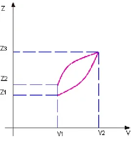
Figure 1.1: Continuous hysteresis loop.
Figure 1.1 describes the state of a system which is characterized by two scalar variables u and w depending in a continuous way on time. We will call them also input and output of the system. We have the following: if the input increases from a to b then the couple (u, w) moves along the
1 Hysteresis operators
curve ABC, on the other hand, if the input decreases from b to a then the couple input-output stays on the curve CDA. If moreover at a certain instant t such that a < u(t) = c < b the input u inverts its movement, then (u, w) moves into the interior of the region bounded by the major loop ABCDE in a suitable way described by the specific model, for example this can be along the curve EF as in the picture.
This means that at any instant t the value of the output w(t) is not simply determined by the value u(t) of the input at the same instant, but it depends also on the previous evolution of the input u. This is the memory effect.
On the other hand we may also require that the path of the couple (u(t), w(t)) is invariant with respect to any increasing time homeomorphism, that is there is no dependence on the derivative of u. This property is named rate independence and it is this fact that allows us to draw the characteristic pictures of hysteresis in the (u, w)−plane, if this did not hold we could not give a graphic representations of the hysteresis loop as the path of the couple would also depend on its velocity.
Even if hysteresis has been known and studied since the end of the eighteenth century, it was only more or less thirty-five years ago that, dealing with plasticity, a small group of Russian mathematicians introduced the concept of hysteresis operator and started a systematic investigation of its properties. The pioneers in this new field were certainly Krasnosel’ski˘ı and Pokrovski˘ı with their important monograph [23]. From that moment onward many scientists coming also from different areas have contributed to the mathematical study of hysteresis. At this purpose we can certainly quote the recent monographes devoted to this topic, see Brokate and Sprekels [11], Krejˇc´ı [25], Mayergoyz [30] and Visintin [39], together with the references therein.
1.1. Hysteresis operators: basic properties
The evolution u 7→ w we briefly outlined before can be formalized by the introduction of the concept of hysteresis operator. This is what Krasnosel’ski˘ı and Pokrovski˘ı did in 1970, dealing with a particular case. This event can be certainly regarded as the beginning of the mathematical theory of hysteresis as the concept of hysteresis operator acting among Banach spaces of time dependent functions is of basic importance in treating the mathematical aspects of several hysteresis models.
In many cases the state of the system is completely described by the couple (u, w) input-output. At any instant t, the output w(t) will depend on the evolution of the input until that time t and also on the initial state of the system. So the initial value (u(0), w(0)) or some equivalent information must be specified. As u(0) is already contained in u|[0,t], we say that in these cases
1.1 Hysteresis operators: basic properties the state of the system can be described by an operator of the following type
F : Dom (F) ⊂ C0([0, T ]) × R → C0([0, T ]) (u, w0) 7→ w(·) := [F(u, w0)](·). (1.1.1)
This is the case, for example, of plays and stops operators (see Section 1.2).
However there are also cases in which the state of the system is not completely characterized by the couple (u, w) but there is also the presence of a variable η ∈ X where X is some suitable metric space; in these situations the state of the system is described by an operator of the following type
F : Dom (F) ⊂ C0([0, T ]) × X → C0([0, T ]) (u, η0) 7→ w(·) := [F(u, η0)](·), (1.1.2)
where η0 ∈ X contains all the information about the initial state. This is the case for example
of the Prandtl-Ishlinski˘ı operators of play or stop type or the Preisach operators (see Sections 1.3 and 1.5).
Operators of type (1.1.1) and (1.1.2) usually fulfill some properties, useful when dealing with P.D.E.s. We now make explicit some of these properties, which can be written without mod-ifications for both operators of type (1.1.1) and (1.1.2). There are also properties which have to be presented in a different way for the two different types of operators (i.e. the semigroup
property) but we will not quote them as we will not need them in the following.
We start with the causality property and rate independence property which
respec-tively read
∀ (u1, w0), (u2, w0) ∈ Dom (F), ∀ t ∈ (0, T ],
if u1 = u2 in [0, t], then [F(u1, w0)](t) = [F(u2, w0)](t),
(1.1.3)
∀ (u, w0) ∈ Dom (F), ∀ t ∈ (0, T ], if s : [0, T ] → [0, T ] is an
increasing homeomorphism, then [F(u ◦ s, w0)](t) = [F(u, w0)](s(t)). (1.1.4)
An operator fulfilling (1.1.3) and (1.1.4) is said to be a hysteresis operator.
In the following we will work with hysteresis operators that are continuous in the following
sense ∀ {(un, w0n) ∈ Dom (F)}n∈N, if un → u uniformly in [0, T ] and w0n→ w0,
then F(un, w0n) → F(u, w0) uniformly in [0, T ]
(1.1.5)
or with operators which are order preserving, that is
∀ (u1, w10), (u2, w02) ∈ Dom(F), ∀ t ∈ (0, T ], if u1 ≤ u2 in [0, t] and w01 ≤ w20,
then [F(u1, w01)](t) ≤ [F(u2, w02)](t).
1 Hysteresis operators
Moreover for an operator F it is also natural to require the following property, usually named piecewise monotonicity preservation (or briefly piecewise monotonicity)
∀ (u, w0) ∈ Dom(F), ∀ [t
1, t2] ⊂ [0, T ],
if u is either nondecreasing or nonincreasing in [t1, t2], then so is F(u, w0).
(1.1.7) Another interesting property is the piecewise Lipschitz continuity property
∃ LF > 0 : ∀ (v, w0) ∈ Dom(F), ∀ [t1, t2] ⊂ [0, T ] if v affine in [t1, t2], then |[F(v, w0)](t2) − [F(v, w0)](t1)| ≤ LF|v(t2) − v(t1)|. (1.1.8) We remark that, if F : Dom(F) ⊂ C0([0, T ]) × X → C0([0, T ]) is a Lipschitz continuous
hysteresis operator with Lipschitz constant LF, then it can be proved that F fulfills (1.1.8).
This implication can be justified in the following way: let us take a function v affine in [t1, t2]
and let us consider a function ¯v : [t1, t2] → R defined as follows: ¯v(t) = v(t1) for all t ∈ [t1, t2].
Then, as ¯v is constant in [t1, t2] then also F(¯v, w0) is constant in [t1, t2] due to the fact we
assumed F to be rate independent; moreover F(v, w0)(t
1) = F(¯v, w0)(t1) as F is also a causal
operator. These facts imply that
|[F(v, w0)](t1) − [F(v, w0)](t2)| ≤ |[F(v, w0)](t1) − [F(¯v, w0)](t1)|
+ |[F(¯v, w0)](t1) − [F(¯v, w0)](t2)| + |[F(¯v, w0)](t2) − [F(v, w0)](t2)|
≤ LF||v − ¯v||C0([0,T ]) = LF|v(t2) − ¯v(t2)| = LF|v(t2) − v(t1)|.
So property (1.1.8) is achieved.
1.2. Scalar play and stop
In this section and in the following ones, we would like to recall some important examples of hysteresis operators; our excursion is far to be deep and complete. We just outline some properties and remarks we will need in the following chapters. For more details on this topic, see the monographs we quoted in the very beginning of the chapter.
1.2.1. The play
The first simple model of hysteresis we consider is a mechanism which is known as play. More precisely we have two elements, A and B which move along a horizontal line with one degree of freedom (see Figure 1.2).
1.2 Scalar play and stop
Figure 1.2: Play between two mechanical elements.
The motion of the two elements can be described as follows: the position w(t) of the middle point of element B remains constant as long as the element A, represented by its end-position
u(t), moves in the interior region of width 2r which is the diameter of the element B. When u hits the boundary of the element B then w moves with the velocity ˙w = ˙u which is direct
outwards. The input-output behaviour is given by the hysteresis diagram which is shown in Figure 1.3.
Figure 1.3: Hysteresis behaviour of the mechanical play.
On the other hand this relation u 7→ w can be also expressed by means of a hysteresis operator. In fact, for any piecewise monotone input function u : [0, T ] → R the output function w(t) :=
1 Hysteresis operators
Pr(u) can be defined by induction using the following formula:
w(0) = max{u(0) − r, min{u(0) + r, 0}}
w(t) = max{u(t) − r, min{u(t) + r, w(tn−1)}} for tn−1 < t ≤ tn, 1 ≤ n ≤ N
where 0 = t0 < t1 < · · · < tN = T is a partition of the time interval [0, T ] such that the
input function u is monotone on each subinterval [tn−1, tn]. The operator Pr is called play
operator.
1.2.2. The stop
Let us consider a device constituted by an elastic element put in series with a plastic one (see Figure 1.4).
Figure 1.4: Prandtl’s model of elasto-plasticity or stop.
It is simple to see that also the relation between the strain and the stress provides another example of hysteresis phenomena (see also Section 1.4). Let us denote by r > 0 a fixed threshold (depending on the characteristics of the bodies and on the materials in contact), which represents the yield stress. As long as the modulus of the stress w is smaller than r, the strain u and the stress w are related through the linear Hooke law. In the case when the yield value has been reached by w, then the stress remains constant under a further growth of u. The elastic behaviour is then recovered once that the strain decreases again. Figure 1.5 describes this situation in a very simplified way. Also in this case it is possible to represent the strain-stress relation by means of a hysteresis operator. More precisely, we still consider a partition 0 = t0 < t1 < · · · < tN = T of the time interval [0, T ] such that the input function
u is monotone on each subintervals [tn−1, tn]. Then the output function w(t) := Sr(u) can be
defined by induction using the following formula:
w(0) = min{r, max{−r, u(0)}}
w(t) = min{r, max{−r, u(t) − u(tn−1) + w(tn−1)}} for tn−1< t ≤ tn, 1 ≤ n ≤ N.
1.2 Scalar play and stop
Figure 1.5: Hysteresis behaviour of the stop.
1.2.3. Play and stop operators with general initial value
In Subsections 1.2.1 and 1.2.2 we introduced the play operator Pr and the stop operator Sr.
More in general, for any initial value w0 we may define for any piecewise monotone input
function u : [0, T ] → R the output function w(t) := Pr(u, w0) inductively using the following
formula:
w(0) = max{u(0) − r, min{u(0) + r, w0}}
w(t) = max{u(t) − r, min{u(t) + r, w(tn−1)}} for tn−1< t ≤ tn, 1 ≤ n ≤ N.
(1.2.1) The following result (see [11], Example 2.2.13 and Theorem 2.3.2; see also [23], Section 2) holds Theorem 1.2.1. For any r ≥ 0, the operator Pr can be extended to a unique Lipschitz
con-tinuous operator Pr : C0([0, T ]) × R → C0([0, T ]) (with Lipschitz constant 1). In addition this
operator Pr is causal and rate independent in the sense of (1.1.3) and (1.1.4), i.e. it is a
hysteresis operator, and moreover it is order preserving and piecewise monotone in the sense of (1.1.6) and (1.1.7).
The same can be done for the stop operator; in fact, for any initial value w0 we may define for
any piecewise monotone input function u : [0, T ] → R the output function w(t) := Sr(u, w0)
inductively using the following formula:
w(0) = min{r, max{−r, u(0) − w0}}
w(t) = min{r, max{−r, u(t) − u(tn−1) + w(tn−1)}} for tn−1 < t ≤ tn, 1 ≤ n ≤ N.
1 Hysteresis operators
The following result is an immediate consequence of Theorem 1.2.1 (see [11], Proposition 2.3.4) Proposition 1.2.2. For any r ≥ 0, the operator Sr can be extended to a unique Lipschitz
con-tinuous operator Sr : C0([0, T ]) × R → C0([0, T ]) (with Lipschitz constant 2, which is optimal).
In addition it turns out that this operator Sr is causal and rate independent in the sense of
(1.1.3) and (1.1.4), i.e. it is a hysteresis operator, and moreover it is piecewise monotone in
the sense of (1.1.7).
It is interesting to notice that the play and the stop operators are closely related, even if the corresponding models describe different situations. The simple relation is the following, which can be checked by direct computation (see also [11], Proposition 2.3.4)
Pr(u, w0) + Sr(u, w0) = I(u) ∀ u ∈ C0([0, T ]), ∀ w0 ∈ R,
where I is the identity operator.
1.2.4. Play and stop operators: a different approach
The play and the stop operators can be introduced also in another way. Let us come back to the classical Prandtl’s model of elasto-plasticity, i.e. to the stop model. Assume that the device (an elastic and a plastic element in series) is composed by a heavy body connected to a spring which has only one degree of freedom (the horizontal line). If a longitudinal force is applied to the spring (which transmits this force to the body), the elongation uE is proportional to the
force w in the following way: uE = σw where σ is a positive constant. Moreover, assuming
Coulomb’s friction law, as we said before there exists a threshold r > 0 (depending on the physical characteristics of the body and of the materials in contact) such that ˙uP = 0 if
|w| < r, ˙uP ≥ 0 if w = r and ˙uP ≤ 0 if w = −r, where uP is the displacement of the body.
This is equivalent to the following variational inequality
|w| ≤ r duP
dt (w − ϕ) ≥ 0 ∀ ϕ : |ϕ| ≤ r.
Summing up, if we denote by u the displacement of the point A in Figure 1.4 then u = uE+ uP
and the previous considerations yield
|w| ≤ r µ du dt − σ dw dt ¶ (w − ϕ) ≥ 0 ∀ ϕ : |ϕ| ≤ r.
The analogous thing can be done for the play, we will see in Section 1.4 that the relation u 7→ w can be expressed by the following variational inequality
|u − w| ≤ r dw
1.2 Scalar play and stop On the other hand it is not difficult to show (see [25], Section I.3) that the following system
(i) |xr(t)| ≤ r ∀t ∈ [0, T ],
(ii) ( ˙u(t) − ˙xr(t)) (xr(t) − ϕ) ≥ 0 a.e. ∀ ϕ ∈ [−r, r],
(iii) xr(0) = x0r
(1.2.3)
admits a unique solution xr ∈ W1,1(0, T ) for any given input function u ∈ W1,1(0, T ) and any
given initial condition x0
r ∈ [−r, r]. Then the stop and the play operators Sr, Pr : [−r, r] ×
W1,1(0, T ) → W1,1(0, T ) can be introduced as solution operators of Problem (1.2.3) by the
formula
Sr(x0r, u) := xr Pr(x0r, u) := u − xr.
It turns out that Theorem 1.2.1 and Proposition 1.2.2 are still valid also in this case. The set Z := [−r, r] is called the characteristic of the operators Sr and Pr. In this case it is a
symmetric one-dimensional set but there are also other possibilities in which one considers tensorial extensions of the play and stop operators, or situations in which one deals with more general closed convex sets as characteristics.
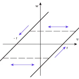
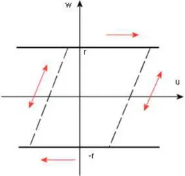
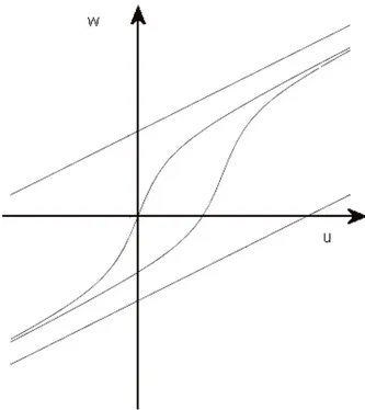
Moreover, both models can be generalized in several ways, for instance if f is a strictly monotone continuous function R → R the relation u 7→ f (w) corresponds for both cases to diagrams similar to Figures 1.3 and 1.5. In the case of the play the hysteresis region is bounded by two parallel nonlinear exterior curves; in the case of the stop the hysteresis region is spanned by a family of parallel nonlinear curves. For more details on the topic, we refer to [39], Sections III.2 and III.3.
Finally we observe that (see [25], Section II.1, Remark 1.3) it is particularly easy to solve Prob-lem (1.2.3) if the input is monotone in an interval [t1, t2] ⊂ [0, T ]. What we get is nothing but
formula (1.2.2) contained in Subsection 1.2.3, which provides therefore an equivalent definition for the operator Sr.
1.2.5. Memory of the play system
Consider a system in which the output depends with hysteresis on the input. This means that the output w(t) at any instant t will depend on the evolution of the input until that time t and also on the initial state of the system. Therefore, in this situation the state of the system can be described by an operator F of type (1.1.2).
Suppose now that F ≡ Pr, the scalar play with characteristic [−r, r]. Then for any given input
function u ∈ W1,1(0, T ) and any given initial condition x0
r ∈ [−r, r] we have
1 Hysteresis operators
We notice that we can associate to any r ∈ R the corresponding value x0
r; this suggests the
idea of making the initial configuration of the play system independent of the initial conditions
{x0
r}r∈R for the output function by the introduction of some suitable function of r. More
precisely, following [25] Section II.2, let us consider any function λ ∈ Λ where Λ := ½ λ ∈ W1,∞(0, ∞); ¯ ¯ ¯ ¯dλ(r)dr ¯ ¯ ¯ ¯ ≤ 1 a.e. in [−r, r] ¾ .
We also introduce some useful subspaces of Λ, i.e.
ΛR := {λ ∈ Λ; λ(r) = 0 for r ≥ R}, Λ0 :=
[
R>0
ΛR. (1.2.4)
Λ is called configuration space and the functions λ are called memory configurations. If Qr : R → [−r, r] is the projection
Qr(x) := sign (x) min{r, |x|} = min{r, max{−r, x}},
then we set
x0
r := Qr(u(0) − λ(r)).
This implies that the initial configuration of the play system only depends on λ and u(0). The same can be done for the initial configuration Sr(x0r, u)(0) := x0r of the stop operator.
We introduce the following more convenient notations
℘r(λ, u) := Pr(x0r, u) sr(λ, u) := Sr(x0r, u), (1.2.5)
for any λ ∈ Λ, for any u ∈ C0([0, T ]) and r > 0, where P
r(x0r, u) and Sr(x0r, u) are then defined
by induction starting from Pr(x0r, u)(0) and Sr(x0r, u)(0) according to (1.2.1) and (1.2.2).
From now on throughout this subsection we will deal only with the play operator. We then set for the sake of completeness ℘0(λ, u) = u. It turns out that the operator ℘r: Λ × C0([0, T ]) →
C0([0, T ]) is Lipschitz continuous in the following sense (see [25], Section II.2, Lemma 2.3)
Lemma 1.2.3. For every u, v ∈ C0([0, T ]), every λ, µ ∈ Λ and r > 0 we have
||℘r(λ, u) − ℘r(µ, v)||∞ ≤ max{|λ(r) − µ(r)|, ||u − v||∞}.
The introduction of the function λ plays an important role in the characterization of the memory of the play system, in the sense that, for any given λ, we can construct the play operator ℘r(λ, u) starting from λ and from a sequence of values (tj, rj) which is the so called
(reduced) memory sequence (see [25], Section II.2 or [39], Section III.6) of any input u at a
certain instant t with respect to the initial configuration λ. These values are what one simply has to know in order to evaluate the output of the play operator.
1.2 Scalar play and stop More precisely, for any u ∈ C0([0, T ]), λ ∈ Λ
0, t ∈ [0, T ] we put ¯ r := max{min{r ≥ 0 : |u(τ ) − λ(r)| = r}, τ ∈ [0, t]}
¯t := max{τ ∈ [0, t] : min{r ≥ 0 : |u(τ) − λ(r)| = r} = ¯r},
and also t0 := ¯t, r0 := ¯r if u(¯t) = λ(¯r) − ¯r, t1 := ¯t, r1 := ¯r if u(¯t) = λ(¯r) + ¯r; (1.2.6) at this point we continue recursively by setting
t2j+1 := max{τ ∈ [t2j, t] : u(τ ) = max{u(σ) : σ ∈ [t2j, t]}}, j = 1, 2, . . .
t2j := max{τ ∈ [t2j−1, t] : u(τ ) = min{u(σ) : σ ∈ [t2j−1, t]}}, j = 1, 2, . . .
rj+1:= (−1) j
2 (u(tj+1) − u(tj)), j = 1, 2, . . .
(1.2.7)
and this procedure goes on until t2j+1 = t or t2j = t for some j.
The (reduced) memory sequence {(tj, rj)} (in symbols RMSλ(u)(t)) can be infinite, and in
such a case
u(t) = lim
j→∞u(tj), j→∞lim rj = 0,
but it can also be finite, and in this case t = tn for some n ∈ N and we put rj := 0 for j ≥ n+1.
The important result we can state is the following (it is proved in [25], Section II.2).
1 Hysteresis operators
Proposition 1.2.4. Let u ∈ C0([0, T ]), λ ∈ Λ
0, r > 0 and t ∈ [0, T ] be given, and let
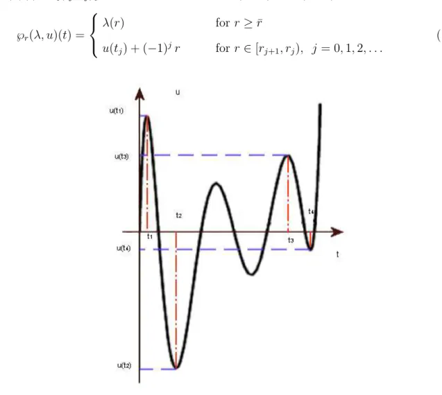
RM Sλ(u)(t) = {(tj, rj)} be the memory sequence (1.2.6) and (1.2.7). Then we have
℘r(λ, u)(t) = λ(r) for r ≥ ¯r u(tj) + (−1)jr for r ∈ [rj+1, rj), j = 0, 1, 2, . . . (1.2.8)
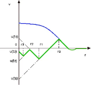
Figure 1.7: Picture illustrating the construction of the reduced memory sequence. Figure 1.6 is explicative of this construction, the curve above represents any given memory configuration λ, the other curve represents the play operator ℘r(λ, u) as r varies (the two lines
coincide from r0 onward in agreement with (1.2.8)). Formula (1.2.8) shows that the
increas-ing sequence {u(t2j)} of local minima and decreasing sequence {u(t2j+1)} of local maxima is
precisely what the system keeps in memory. The output values are determined only by these sequences and all the rest of the input history is irrelevant. Figure 1.7 also shows the construc-tion of the reduced memory sequence. This memory sequence is also called reduced because in reality for any continuous piecewise monotone function u : [0, T ] → R and any t ∈ [0, T ] we can also consider the finite sequence of instants {tj} for j = 1, . . . , n of the time interval [0, t] at
which the function u inverts its monotonicity. The finite sequence of the corresponding values
1.3 Prandtl-Ishlinski˘ı operators or [39], Section III.6) of the function u at any instant t. This sequence determines the value at
t of any hysteresis operator applied to u as any hysteresis operator is also rate independent.
The fact that the RMS is mostly used in applications is due to the fact that the CMS (which can be finite or infinite for a given input function not necessarily piecewise monotone) does not necessarily exist for any continuous or even infinitely differentiable function, whereas the
RM S exists for any continuous function and this entails important consequences in the study
of a large class of hysteresis models.
We conclude this section with the following lemma - which can be found for example in [26], Chapter 4 - and which adds some information to the previous proposition.
Lemma 1.2.5. Let w ∈ C(R+) (where C(R+) is the space of continuous functions on R+) and
let t ≥ 0 be given. Set
wmax(t) = sup
τ ∈[0,t]
w(τ ), wmin(t) = inf
τ ∈[0,t]w(τ ).
Then for all λ ∈ Λ and r > 0 we have
℘r[λ, w](τ ) ≤ max{λ(r), wmax(t) − r} ∀ τ ∈ [0, t]
℘r[λ, w](τ ) ≥ min{λ(r), wmin(t) + r} ∀ τ ∈ [0, t]
℘r[λ, w](t) = λ(r) for r > ||mλ(w(·))||[0,t],
where for v ∈ R we put mλ = inf{r ≥ 0; |λ(r) − v| = r}.
1.3. Prandtl-Ishlinski˘ı operators
1.3.1. Definition and basic properties
The Prandtl-Ishlinski˘ı operators (of play and stop type) are more complex models than the ones just introduced. In Section 1.4 we will show a rheological construction of these models, i.e. we will present them as models of elasto-plasticity (with strain hardening) obtained by combining arbitrary families of stops and plays in series and in parallel. At this stage we adopt the following definition which includes both concepts. The two definitions (this one and the one contained in Section 1.4) are, of course, equivalent in the sense that they represent the same hysteresis models.
Definition 1.3.1. Suppose that a constant a ≥ 0 and a function h ∈ BVloc(0, ∞) are given,
such that lim
s→0+h(s) = a. We set
ϕ(r) :=
Z r
0
1 Hysteresis operators
Then the operator Fϕ : Λ0× C0([0, T ]) → C0([0, T ]) defined by the formula
Fϕ(λ, u) = a u +
Z ∞
0
℘r(λ, u) dh(r), λ ∈ Λ0, u ∈ C0([0, T ]) (1.3.1)
where ℘r is the play operator (1.2.5) and Λ0 is introduced in (1.2.4), is called
Prandtl-Ishlinski˘ı operator generated by the function ϕ which is then called the generator of Fϕ.
The Stieltjes integral in (1.3.1) is finite as λ ∈ Λ0 and this implies, as we saw in Proposition
1.2.4, that ℘r(λ, u) vanishes for r sufficiently large. The distinction between Prandtl-Ishlinski˘ı
operators of stop type and play type can be characterized in terms of the generator, i.e. a
convex function ϕ generates an operator of play type, a concave function ϕ generates instead
an operator of stop type.
Theorem 1.2.1 implies the following result.
Theorem 1.3.2. The operator Fϕ is causal and rate independent in the sense of (1.1.3) and
(1.1.4), i.e. it is a hysteresis operator; moreover if the function h is nonnegative and monotone,
then Fϕis piecewise monotone in the sense of (1.1.7). Finally Fϕis locally Lipschitz continuous
in the following sense: for all t ≥ 0, for all w1, w2 ∈ C0([0, T ]), for all λ1, λ2 ∈ ΛR, where R > 0
is given |Fϕ(λ1, w1) − Fϕ(λ2, w2)| ≤ |h(0)| |w1(t) − w2(t)| + ¡Var[0,R(t)]h ¢ max©||λ1(r) − λ2(r)||[0,R], ||w1− w2||C0([0,t]) ª where R(t) := max{R, ||w1||C0([0,t]), ||w2||C0([0,t])}.
1.3.2. Further properties and energy inequalities
The variational character of the Prandtl-Ishlinski˘ı operators leads to natural properties for absolutely continuous inputs. More precisely we can state the following result which can be found in [25], Section II.4.
Theorem 1.3.3. Let h : [0, ∞) → [0, ∞) be a monotone function. For u1, u2 ∈ W1,1(0, T ),
λ1, λ2 ∈ Λ0 and r > 0 put ξr(i) := pr(λi, ui), xr(i) := ui − ξ(i)r , wi := Fϕ(λi, ui) = h(0)ui +
R∞ 0 ξ (i) r dh(r), i = 1, 2, ˜u := u1− u2, ˜w := w1 − w2, ˜ξr:= ξr(1)− ξr(2), ˜x := x(1)r − x(2)r . Then ˙˜ w(t)˜u(t) ≥ 1 2 d dt[h(0)˜u 2(t) + Z ∞ 0 ˜ ξ2 r(t)dh(r)] a.e. if h is nondecreasing (1.3.2) ˜ w(t) ˙˜u(t) ≥ 1 2 d dt[h(∞)˜u 2(t) − Z ∞ 0 ˜ x2 r(t)dh(r)] a.e. if h is nonincreasing,
1.3 Prandtl-Ishlinski˘ı operators where, from now on (in the case these quantities exist)
h(0) = lim
s→0h(s); h(∞) := lims→∞h(s). (1.3.3)
The following result gives us explicit energy dissipation formula for the Prandtl-Ishlinski˘ı op-erators (1.3.1) (see [25], Section II.4, Proposition 4.6)
Proposition 1.3.4. Let R > 0, λ ∈ ΛR, u ∈ W1,1(0, T ) be such that ||u||∞ ≤ R and consider
a given non-negative function h ∈ BVloc(0, ∞). For r > 0 we put ξr := ℘r(λ, u), xr := u − ξr.
Then we have the following two cases:
• (Prandtl-Ishlinski˘ı operators of play type) if h is nondecreasing and w := h(0) u + Z ∞ 0 ξrdh(r), U := 1 2h(0) u 2+1 2 Z ∞ 0 ξr2dh(r), D := Z ∞ 0 r ξrdh(r), (1.3.4) then we have ˙
w(t) u(t) − ˙U(t) = | ˙D(t)| a.e. in (0, T );
• (Prandtl-Ishlinski˘ı operators of stop type) if h is nonincreasing and w := h(∞) u − Z ∞ 0 xrdh(r), U := 1 2h(∞) u 2− 1 2 Z ∞ 0 x2 rdh(r), D := − Z ∞ 0 r ξrdh(r), then we have
w(t) ˙u(t) − ˙U(t) = | ˙D(t)| a.e. in (0, T ).
This result can be interpreted by saying that the Prandtl-Ishlinski˘ı operators of play and stop type are thermodynamically consistent. Here the quantity ˙w(t) u(t) or the quantity w(t) ˙u(t) is the power density, U is the internal energy density and finally | ˙D| is the dissipation
rate which is positive in agreement with the Second Principle of Thermodynamics.
For the last result of this subsection we restrict ourselves to the case of Prandtl-Ishlinski˘ı operators of play type, i.e. we assume that the function h is positive and nondecreasing in (0, ∞).
Besides the energy inequality stated by the previous proposition, the Prandtl-Ishlinski˘ı oper-ators of play type admit a higher order energy inequality which can be summarized in
¨
w(t) ˙u(t) − ˙V (t) ≥ 0 in the sense of distributions where w is the same as in (1.3.4) and where
V (t) = 1
2w(t) ˙u(t)˙ a.e. in [0, T ]. (1.3.5) First we introduce the concept of trajectory (which can be found i.e. in [25], Section II.4).
1 Hysteresis operators
Definition 1.3.5. Let F : C0([0, T ]) → C0([0, T ]) be a rate independent operator and let u ∈
C0([0, T ]) be a function which is monotone (nonincreasing or nondecreasing) in [t
1, t2] ⊂ [0, T ],
with u(ti) = ui, for i = 1, 2. Then there exists a function Φ : Conv{u1, u2} → R such that
F(v)(t) = Φ(v(t)) for all t ∈ [t1, t2] and for every function v ∈ C0([0, T ]) which is monotone in
[t1, t2] and v(t) = u(t) for t ∈ [0, T ] \ (t1, t2). If moreover F is continuous, then Φ is continuous
and if F is locally monotone on absolutely continuous inputs, then Φ is nondecreasing and absolutely continuous. The function Φ is called trajectory of F along u in [t1, t2].
Now we state here the precise statement of the so called second order energy inequality, for more details see for example [25], Section II.4, Theorem 4.19.
Theorem 1.3.6. Let F : C0([0, T ]) → C0([0, T ]) be a continuous and rate independent operator.
Assume that there exist constants R > 0, bR > aR ≥ 0 and KR ≥ 0 such that, for every
u ∈ C0([0, T ]) with ||u||
∞ ≤ R, the trajectory Φ of F along u in a monotonicity interval [t1, t2]
has the following properties:
(i) Φ is absolutely continuous in J := Conv{u(t1), u(t2)}, aR ≤ Φ0(v) ≤ bR for a.e. v ∈ Int J;
(ii) if u is nondecreasing in [t1, t2], then Φ(v) −
1 2KRv
2 is convex in J;
(iii) if u is nonincreasing in [t1, t2], then Φ(v) +
1 2KRv
2 is concave in J.
Let u ∈ W1,∞(0, T ) be a given function such that ||u||
∞ ≤ R and w := F(u) ∈ W2,1(0, T ).
Then:
(a) the function V (t) introduced in (1.3.5) belongs to BV (0, T ) and aR 2 ˙u 2(t) ≤ V (t) ≤ bR 2 ˙u 2(t) a.e.; (b) Z t s ¨ w(τ ) ˙u(τ ) dτ −V (t)+V (s) ≥ 1 2KR Z t s
| ˙u(τ )|3dτ for almost all 0 < s < t < T . (1.3.6)
The following proposition ([25], Section II.4) then allows us to verify that the previous theorem can be actually applied to Prandtl-Ishlinski˘ı operators of play type
Proposition 1.3.7. Let h ∈ BVloc(0, ∞) be a given nonnegative function and let F := Fϕ(λ0, ·)
be the Prandtl-Ishlinski˘ı operator (1.3.1) for some R > 0 and λ0 ∈ ΛR. Set
H−(R) := inf ½ h(b) − h(a) b − a ; 0 < a < b < R ¾ .
If H−(R) ≥ 0 then the hypothesis of Theorem 1.3.6 are satisfied for KR :=
1
1.4 Rheological models
1.4. Rheological models
Rheology is the study of mechanical constitutive properties of materials; rheology usually defines
some ideal bodies which are constructed by the combination in series and in parallel of a small class of primitive elements which correspond to the main mechanical properties such as elasticity, viscosity, plasticity and so on. This primitive bodies are characterized by a constitutive relation between macroscopic strain and stress tensors ε and σ respectively. For more details on this topic we refer to [39] Chapters II and III or also [38].
From now on we confine ourselves to the one-dimensional scalar case and we present some classes of rheological models. We recall that if two or more either elementary or composed rheological models are coupled in series, they experience the same stress which is also the stress of the composed model while the strain of the global model is the sum of their strains
σ = σ1 = σ2 = . . . ; ε = ε1+ ε2 + . . . ;
on the other hand, for the combination in parallel these properties shared by stress and strain tensors are interchanged
ε = ε1 = ε2 = . . . ; σ = σ1+ σ2 + . . . .
If A1 and A2 are two either elementary or composite models we will denote by the rheological
formula A1− A2 or A1|A2 respectively the combination in series and in parallel of A1 and A2.
We can also extend in an easy way these rules to the case when we are combining infinite elements. In this case, let (P, A, µ) be a measure space with µ a finite non negative measure and let {Aρ}ρ∈P be a family of rheological elements. Their combination in series and in parallel,
respectively denoted by X
ρ∈P
Aρ and
Y
ρ∈P
Aρ correspond to the following relations
σI = σρ µ a.e. in P εI = Z P ερdµ(ρ) εI = ερ µ a.e. in P σI = Z P σρdµ(ρ),
where εI and σI represent the strain and the stress of the global model while ερand σρare the
strain and the stress of the single rheological element.
Throughout this section we will mainly refer to two basic elements, an elastic and a plastic element, respectively denoted by E and P, which correspond to the constitutive laws of the form
ε = α(σ) or σ = β(ε),
1 Hysteresis operators
where α and β := α−1 are continuous real functions and I
Z is the indicator function of a
non-empty closed, convex set Z ⊂ R; we assume that α(0) = 0 and 0 ∈ Z.
Ü elastic and plastic elements in parallel E|P . We consider the model obtained by combining an elastic and a plastic element in parallel. This model is usually called play (see also Section 1.2 for an equivalent definition) and corresponds to the rheological law
σ ∈ β(ε) + (∂IZ)−1( ˙ε) or equivalently ˙ε ∈ ∂IZ(σ − β(ε))
which is also equivalent to the following variational inequality
σ − β(ε) ∈ Z, ˙ε[σ − β(ε) − v] ≥ 0 ∀ v ∈ Z;
we introduce also the initial condition
ε(0) = ε0
and require that σ and ε0 fulfill the compatibility condition σ(0) − β(ε0) ∈ Z.
It can be easily shown that in this case the relation σ 7→ ε can be expressed in the form
ε(t) = [P(σ, ε0)](t) in [0, T ] where
P : C0([0, T ]) × R → C0([0, T ])
is a causal and rate independent operator (so a hysteresis operator) in the sense of (1.1.3) and (1.1.4). Moreover P is also continuous in the sense of (1.1.5) and Lipschitz continuous, i.e. there exists a constant LP such that, for all σ1, σ2 ∈ C0([0, T ]) and for all ε01, ε02 ∈ R
||P(σ1, ε01) − P(σ2, ε02)||C0([0,T ]) ≤ LP(||σ1− σ2||C0([0,T ])+ |ε01− ε02|).
The play operator which comes from this construction is equivalent to the play operator intro-duced in Subsection 1.2.4 if β(ε) = ε.
Ü elastic and plastic elements in series E − P . Now let us consider the model obtained by combining an elastic and a plastic element in series. This model is usually called prandtl model or stop (see also Section 1.2 for an equivalent definition) and corresponds to the rheological law
˙ε ∈ α(σ)˙+ ∂IZ(σ)
which is equivalent to the following variational inequality
1.4 Rheological models we introduce also the following initial condition
σ(0) = σ0.
It is not difficult to see that in this case the relation ε 7→ σ can be expressed in the form
σ(t) = [S(ε, σ0)](t) in [0, T ]
where
S : C0([0, T ]) × R → C0([0, T ])
is a causal and rate independent operator (so a hysteresis operator) in the sense of (1.1.3) and (1.1.4). Moreover S is also continuous in the sense of (1.1.5) and Lipschitz continuous, i.e. there exists a constant LS such that, for all ε1, ε2 ∈ C0([0, T ]) and for all σ10, σ02 ∈ R
||S(ε1, σ10) − S(ε2, σ02)||C0([0,T ]) ≤ LS(||ε1− ε2||C0([0,T ])+ |σ10− σ02|).
The stop operator which comes from this construction is equivalent to the stop operator intro-duced in Subsection 1.2.4 if α(σ) = σ.
ÜQρ∈P(Eρ−Pρ) : parallel combination of elastic and plastic elements in series.
Let us now assume to have a measure space (P, A, µ) where µ is a finite non negative Borel measure, and two families {Eρ}ρ∈P and {Pρ}ρ∈P of elastic and rigid, perfectly plastic elements
fulfilling the following rheological laws
ερ= αρ(σρ) or σρ= βρ(ερ)
˙
ερ∈ ∂IZρ(σρ),
where αρ and βρ = α−1ρ are continuous and strictly monotone functions R → R and IZρ is
the indicator function of a closed interval Zρ. At this point we consider the model obtained
by combining in series a family of plays (i.e. a serial combination of a family of models each composed by an elastic element in parallel with a plastic one). This model is known as Prandtl-Ishlinski˘ı model of play type. Let us see how this model can be represented by means of a hysteresis operator. We know that for any ρ ∈ P, the model obtained by combining in parallel an elastic element Eρ and a plastic one Pρ corresponds to the rheological law
˙ ερ∈ ∂IZρ(σρ− βρ(ερ)) ερ(0) = ε0ρ
and we said before that this system can be also represented by means of a hysteresis operator
1 Hysteresis operators
Thus, the Prandtl-Ishlinski˘ı model of play type corresponds to the following system ˙ ερ∈ ∂IZρ(σI− βρ(ερ)) µ−a.e. in P, ερ(0) = ε0ρ µ−a.e. in P, εI = Z P ερdµ(ρ),
where σI and εI are the strain and the stress of the composite model. Using the fact that for
any ρ ∈ P the corresponding play model can be represented by means of a hysteresis operator, we also have
εI =
Z
P
Pρ(σI, ε0ρ) dµρ=: Iµ(σI, {ε0ρ}ρ∈P).
Remark 1.4.1. Since βρ are increasing functions, we see that ˆερ:= βρ(ερ) are the outputs of
the linear play. Hence,
εI =
Z
P
β−1
ρ (ˆερ) dµ(ρ),
which is essentially nothing but formula (1.5.8) with P = (0, ∞) and g(ρ, v) = µ0(ρ) β−1 ρ (v).
This construction is actually known to be equivalent to the Preisach model for regular measures
µ, see [25], Section II.3, Remark 3.9.
Thus denoting by M(P) the set of measurable functions P → R, we have that
Iµ: C0([0, T ]) × M(P) → C0([0, T ])
is a causal and rate independent operator (so a hysteresis operator) i.e. fulfilling (1.1.3) and (1.1.4) (for more details we refer to [39] Chapters II and III or also [38]). Moreover Iµ is also
continuous in the sense of (1.1.5) and finally
Iµ: C0([0, T ]) × L1(P) → C0([0, T ])
is Lipschitz continuous, in the sense that there exists a constant LI such that, for all σI1, σ2I ∈
C0([0, T ]) and for all ε0 1
ρ , ε0 2ρ ∈ L1(P)
||Iµ(σ1I, ε0 1ρ ) − Iµ(σ2I, ε0 2ρ )||C0([0,T ])≤ LI(||σI1− σI2||C0([0,T ])+ ||ε0 1ρ − ε0 2ρ ||L1(P)).
This operator is equivalent to the Prandtl-Ishlinski˘ı operator introduced in (1.3.1) under suit-able assumptions on the measure µ and on the function h.
Ü Pρ∈P(Eρ|Pρ) Serial combination of elastic and plastic elements in
paral-lel. We now consider the model obtained by combining in parallel a family of stops (i.e. a parallel combination of a family of models each composed by an elastic element in series with
1.4 Rheological models a plastic one). This model is known as Prandtl-Ishlinski˘ı model of stop type. Let us see how this model can be represented by means of a hysteresis operator. We know that for any ρ ∈ P, the model obtained by combining in series an elastic element Eρ and a plastic one
Pρ corresponds to the rheological law
˙ ερ∈ αρ(σ)˙+ ∂IKρ(σρ) σρ(0) = σρ0
and we said before that this system can be also represented by means of a hysteresis operator
Sρ: C0([0, T ]) × R → C0([0, T ]) σρ(t) = Sρ(ερ, σ0ρ)(t).
Thus, the Prandtl-Ishlinski˘ı model of stop type corresponds to the following system ˙ εI ∈ αρ(σρ)˙+ ∂IKρ(σρ) µ−a.e. in P, σρ(0) = σ0ρ µ−a.e. in P, σI = Z P σρdµ(ρ),
where σI and εI are the strain and the stress of the composite model. Using the fact that for
any ρ ∈ P the corresponding stop model can be represented by means of a hysteresis operator, we also have
σI =
Z
P
Sρ(εI, σρ0) dµρ=: Jµ(εI, {σρ0}ρ∈P).
Thus we have that
Jµ: C0([0, T ]) × M(P) → C0([0, T ])
is a hysteresis operator (i.e. a causal and rate independent operator in the sense of (1.1.3) and (1.1.4)) (for more details we refer to [39] Chapters II and III or also [38]). Moreover Jµ is also
continuous i.e. fulfilling (1.1.5) and finally
Jµ : C0([0, T ]) × L1(P) → C0([0, T ])
is Lipschitz continuous, in the sense that there exists a constant LJ such that, for all ε1I, ε2I ∈
C0([0, T ]) and for all σ0 1
ρ , σρ0 2∈ L1(P)
1 Hysteresis operators
1.5. The Preisach operator
1.5.1. Delayed relay
It is the simplest example of discontinuous hysteresis nonlinearity. It is characterized by two thresholds, say ρ1, ρ2 and two output values which we assume to be equal to −1 and +1. For
any couple ρ = (ρ1, ρ2) ∈ R2 with ρ1 < ρ2, the delayed relay operator
hρ : C0([0, T ]) × {−1, 1} → BV (0, T ) ∩ Cr0([0, T )), (1.5.1)
(where BV (0, T ) is the Banach space of functions [0, T ] → R having finite total variation and
C0
r([0, T )) is the linear space of functions which are continuous on the right in [0, T )), can
be defined in the following way: for any u ∈ C0([0, T ]) and any ξ ∈ {−1, +1}, the function
w = hρ(u, ξ) is given by w(0) := −1 if u(0) ≤ ρ1, ξ if ρ1 < u(0) < ρ2, 1 if u(0) ≥ ρ2
and, for any t ∈ (0, T ], setting Wt:= {τ ∈ (0, t] : u(τ ) = ρ1 or ρ2}, by
w(t) := w(0) if Wt = ∅ −1 if Wt 6= ∅ and u(max Wt) = ρ1, 1 if Wt 6= ∅ and u(max Wt) = ρ2.
Thus w is uniquely defined in [0, T ] and has the regularity outlined in (1.5.1). It turns out that the operator hρ is causal, rate independent, order preserving and piecewise monotone in the
sense of (1.1.3), (1.1.4), (1.1.6) and (1.1.7).
We conclude the subsection presenting an interesting connection between the relay and the system of play operators {℘r(λ, u)}r≥0 introduced in (1.2.5).
First of all we give the following definition which will be also useful in the following Definition 1.5.1. The preisach plane
P := {ρ = (ρ1, ρ2) ∈ R2 : ρ1 < ρ2} (1.5.2)
is the set of thresholds of delayed relay operators hρ.
In the following we will often use a different system of coordinates, in order to describe P. For example we can consider the half-width σ1 =
ρ2− ρ1
2 and the mean value σ2 =
ρ1+ ρ2