Performance measurement in mutual fund analysis

(1)

Department of Economics and Finance

Chair in Advanced Corporate Finance

Performance Measurement in Mutual Fund Analysis

Supervisor

Prof. Raffaele Oriani

Candidate

Davide Mancini

Co-Supervisor

Prof. Enrico Maria Cervellati

(2)

ACKNOWLEDGMENTS

I am taking this chance to express my appreciation to everybody who supported me throughout the course of this Master thesis project. I am grateful for their guidance, fruitful criticism, and assistance. I am indebted to them for sharing their enlightening views.

I express my warm thanks to Professor Terrance Odean who sponsored me as a Visiting Scholar at University of California at Berkeley, Haas School of Business.

I would also like to thank my Supervisor and Co-Supervisor, Professor Raffaele Oriani and Professor Enrico Maria Cervellati respectively for their availability in dealing with my issues overseas.

(3)

LIST OF TABLES

Table Page

Table 1: Style Box. Source: Fact Sheet: The Morningstar Style Box ... 13 Table 2: : Fama-French Factor summary statistic... 44 Table 3: Parameters’ P-values percentage significance ... 46

(6)

LIST OF FIGURES

Figure Page

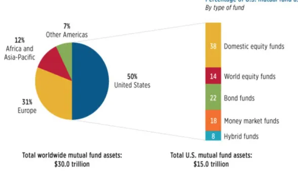
Figure 1: Total Worldwide Mutual Fund assets. Percentage of total net assets, year-end

2013. Source: International Investment Funds Association ... 7

Figure 2: Mutual Fund Assets by Age Group. Percentage of households’ mutual fund assets, selected years. Source: Investment Company institute ... 8

Figure 3: CRSP Funds Specific Example ... 34

Figure 4: Historical Return Histogram ... 44

Figure 5: Mean Error distribution ... 47

(7)

INTRODUCTION

Why should we study mutual funds? They “simply” manage $30 trillion and growing.

Figure 1: Total Worldwide Mutual Fund assets. Percentage of total net assets, year-end 2013. Source: International Investment Funds Association

Mutual funds allow individuals to become investors by creating a system in which funds are pooled and then invested on their behalf in a litany of assets. There are numerous advantages available to investors who entertain the idea of mutual funds. One can buy a mutual fund’s share and gain the same access to a diversified portfolio. This action decreases the amount of risk associated with buying a variety of individual securities.

Mutual fund analysts and managers overcome the large amounts of time and limited resources needed by an individual to optimize the asset allocation. They research information and execute their strategies. Using the Center for Research in Security

Prices (CRSP) Survivor Bias Free US Mutual Fund Database, the following

(8)

Mutual funds broke-out during the ‘80s when they experienced farfetched returns. Despite the introduction of separate account1 and exchange traded funds2_{as valid}

alternatives, the industry is still growing, accounting for a market value for trillions of dollars, with more than ten thousand mutual funds. In spite of the constant growth of the industry, investors’ age distribution is not persistent. As we can see from Figures 2, the “younger than 35” category kept decreasing over the last 20 years, while the others are constant or increasing. Older people manage to save more and their attitude towards investment through mutual funds is extremely good for the outflow if the industry. However, the reduction of younger investors may create concern for the evolution of the market.

Figure 2: Mutual Fund Assets by Age3 Group. Percentage of households’ mutual fund

assets, selected years. Source: Investment Company institute

Throughout the analysis of different risk factors we will identify the finest models to explain mutual fund performance. Moreover, we will test if mutual fund managers posses advantageous skills, which, in theory would allow them to outperform

1

Investment account that a financial advisor uses to buy assets. The financial advisor pools money from different subjects. Differently from the mutual fund case, these subjects do not posses any security.

2_{A derivative traded on an exchange that differently from the mutual fund does not posses any net}

asset value (NAV).

(9)

competitors. Therefore, we will try to answer whether a coefficients time series analysis can, and if so in which case, improve the precision of classical models. The dissertation aims to deliver a precise analysis as well as to clearly convey intuitions and concepts that may be foreign to audiences of differing backgrounds. The Outline is as follow. The literature review delineates an essential mutual funds framework, which the analysis will be drawn upon. In addition, we will discuss the relevant literature with the understanding that this dissertation does not aim to be a mere summary of previous studies. The methodology chapter provides a specific description of the database and how we used it for the analysis. Also, we outline the models used for the 2-step analysis. In the chapter dedicated to the results, we will try to present, in an organized way, the most significant findings, underlying when they match previous literature and when they do not. Finally, we will highlight the innovations of the approach of this work in the conclusive chapter. Taking all into consideration, we aim to produce an intuitive understanding of the results of this research.

(10)

CHAPTER I: Background and Literature Review

This chapter provides an adequate background on the mutual funds environment in order to understand the outline of the analysis. Also, it aims to emphasize the topic’s impact on the modern economy. We will also review the relevant literature in order to produce a framework for the specific models that will be implemented in the following chapters. In order to be as schematic as possible, we will divide the relevant literature in four main sections. The first one is dedicated to the performance measurement methods used by the most influent authors on the subject, the second one on the stock picking and market timing ability studied throughout the performance measurement models studied, the third one is devoted to the investigation of some models proposed in the first section but with a time varying coefficients approach and in the fourth section we will discuss what the money in/outflows from the industry do tell as about the performance measurement.

Mutual Funds Background

Through an expert management service, mutual funds grant individual/institutional investors the chance to buy, in a simple and quick way, a financial product that is characterized by a high level of diversification. However, the mutual fund environment is also characterized by high, direct and indirect, costs, such as entry/exit fees or tax implications.

Investors may invest their money into a variety of funds depending on their constitution or investment objective. Each of these choices allows investors a simplified process to pool funds with other individuals, and thus minimizing financial risk. There are two main ways a mutual fund can be organized:

(11)

An open-ended mutual fund consists of shares that can be easily sold or bought at a daily fixed price, which is the net asset value or NAV. A value calculated at the end of each trading day, it typically reflects the fund's underlying securities. This ease of buying and selling shares is the principal factor of distinction for this type of fund. Open-end funds are divided into stock funds (the majority), bond funds, money market funds and hybrid funds; however, the most important classification, in our opinion, involves their type of activity: they can be active funds, attempting to outperform a certain index, or passive funds, attempting, instead, to replicate an index.

Close-ended funds and exchange-traded funds share similar characteristics, first among them; both can be traded like stocks on a stock exchange. Exactly as for those, they are initially sold with an initial public offering (in this case, investors are usually publicly traded investment companies), and then they are traded on the market at the prevailing market price. Therefore, their shares price is usually different from the NAV and can change throughout the day. As for open-end funds, close-end funds are also classified into stock funds and bond funds.

As stated previously, the majority of mutual funds can be categorized into three main categories — bond funds, also referred to as “fixed income” funds, money market funds, and stock funds, also referred to as “equity funds.” Each type of fund consists of different features, risks, and rewards. In general, actions that warrant a higher risk of loss yield a higher potential return.

(12)

4_{In comparison to other mutual funds, money market funds are associated with low} risks. They abide by specific laws such as; investing in short-term and high-quality investments, which are only issued by U.S. authorities like local and federal governments and national corporations. Money market funds attempt to maintain the net asset value or NAV associated with them at $1.00 for each share. However, the NAV has the potential for its value to drop below $1.00 if the investments of the fund do not perform well. Fortunately, investor losses occur rarely, but they are possible. Money market funds distribute dividends as short-term interest rates. Historically, bond and stock funds have experienced returns that are greater than those found in money market funds. Thus, this situation illustrates how inflation risk within money market funds causes concern for investors.

Bond funds differ from money market funds because there are not required by law to follow the same rules governed by the SEC. This allows them to develop strategies that produce higher yields and also present higher risks. Bond funds are also not restricted to only investing through short-term or high-quality investment possibilities. In addition, there are litanies of bond types, which all have various reward and risk profiles associated to each. Below are three types of risk found with bond funds:

Credit Risk: this addresses the unfortunate circumstance when issuers, the party that possesses the fund’s bonds, cannot repay their debts. However, the possibility of credit risk occurring decreases when bond funds are invested in U.S. treasury bonds or insured bonds. This highlights the importance of

4_{This definition and the following are taken from SEC’s website:}

(13)

investors to pay attention to companies with good credit ratings, thus their investment in that company’s bonds will experience less risk.

Interest Rate Risk: this is associated with the situation of a bond’s market value decreasing when interest rates increase. Unfortunately, all bonds funds are vulnerable to this type of risk, including parties who invest in insured or Treasure bonds. Long-term bonds become a riskier choice for funds to invest in due to their prolonged exposure to the market, thus increasing the probability that their value will decrease.

Prepayment Risk: this occurs when a bond has been paid off earlier than its maturity. In the scenario that interest rates plummet, the bond’s issuer has the option to retire, also known as paying off the bond’s debt. Then, they issue new bonds that are of a lesser market value. Consequently, this lessens the monetary success of the fund because the fund loses its capability to produce a return that is higher or the same as the old bonds.

Stock funds embody the major category of funds. Due to the amount of possible stock categorization the best representation of this mutual fund category is through a style box5 that delivers a graphic illustration of stock fund characteristics.

Table 1: Style Box. Source: Fact Sheet: The Morningstar Style Box Investment Style

Value Blend Growth

Si ze Large Mid Small

5_{This is a proprietary Morningstar data point. The Morningstar Style Box is a nine-square grid that}

provides a graphical representation of the "investment style" of stocks and mutual funds. For stocks and stock funds, it classifies securities according to market capitalization (the vertical axis) and growth and value factors (the horizontal axis) -

(14)

Value/Income funds invest in stocks that can regularly distribute dividends. This category includes index funds, which have the capabilities to achieve equal returns to a specific market index, like the S&P 500 Composite Stock Price Index, through investing in a representative sample or all of the companies included in an index. In riskier circumstances, growth funds target stocks that potentially yield larger capital gains in exchange for the absence of regular dividends. Stocks have been shown to have better long-term performance in comparison to other kinds of investments like corporate bonds, government bonds, and treasury securities. However, taking into account short-term characteristics, a stock’s value can fluctuate over a spectrum of high and low values. There are numerous reasons as to why stock prices can rise and fall such as the overall success of the economy or the theory of supply and demand for specific services. Hence, the market risk poses the greatest potential or gamble for investors in stocks funds.

According to Investment Company Institute (2013), mutual funds come in many other different categories: sector funds6, target-date mutual funds7 and so on. They allow individuals, with differing investing methods, to participate in the market providing convenient specific services. Due to the variety of mutual funds, individuals can easily afford to build a well-diversified portfolio among the different categories. Moreover, their different investment approach allows investors to match risk preferences. Indeed, if an investor believes in active portfolio management, he/she will prefer actively managed funds. In contrast, an investor can also invest in passive funds or index mutual funds that are not affected by manager's presence.

6_{Sector funds may specialize in a particular industry segment, such as technology or consumer}

products stocks

(15)

Mutual funds are easily accessible to all types of investors; the investment process is further made easier when mutual fund companies only require a thousand dollar as minimum entrance investment8. Also, sales load or extra fees are not included when capital gains and dividends are reinvested into their mutual fund. Families of funds bring forward those advantages; they are a collection of different mutual funds that share organizational systems. However, each fund that is included in the family probably has differing investment objectives and executes diverse strategies. Another advantage to “family of funds” remains in funds offering easier avenues of exchange, this allows shareholders to transfer monetary funds easily depending on their change of investment focus and desired exposure to risk.

Similar to how direct deposit works with paychecks, money from a mutual fund can be directly transferred into a personal bank account and vice versa, without charging the individual investor. Despite there being a multitude of investment options available to the individuals, mutual funds offer a simplified process to attain financial goals such as paying off student loans and retirement. Individuals who invest into a mutual fund, also known as mutual fund shareholders, may receive cash equal to the portion they own at that moment if the company goes out of business.

Due to their public availability, mutual funds are also ideal for their transparency, which ensures investor security. Mutual fund companies gain confidence from investors because they must maintain performance track records for all mutual funds they oversee and sustain accurate audits. Plus, the Board of Directors of a mutual fund often employs a new investment advisor if the previous manager does not consider the interests of its financial contributors.

(16)

Mutual Funds in the literature

Since the early ‘70s, countless numbers of researches have been done in order to fully understand and explain the performance of mutual funds and their impact on modern economy. In the attempt of analyzing mutual funds performance, it is critical to discuss the problems concerning standard data sources on funds that the literature has already point out in order to have a clear idea of the framework in which we are working on. In particular, we will address CRSP database, which is one of the main data provider for mutual funds research. Elton, E., Gruber, M. (2011) identify four main problems:

1. Incubator bias: Incubator funds are one of the causes of upward bias in mutual funds returns data. These are funds with limited capital capacity incubated for a certain period by a larger fund. After this period, only the successful funds data are inserted in the database, while the history of failing ones is completely inexistent. There are two ways to deal with this problem, as Evan, R. (2010) suggested: either we eliminate the data of incubator funds before the ticker creation date9, or we eliminate all the first three years10 of data from all funds, even though this implies loosing useful data from non-incubator funds. 2. Backfill (or Selection) bias: Small funds data are usually incomplete. Indeed,

many of them11 need not to report NAV daily or as frequently as bigger funds. Moreover, only successful funds enter standard databases. Removing such data in the analysis can eliminate the biases they create.

9_{A ticker is given to a fund when it becomes public, thus only successful incubator funds obtain one.} 10_{Three years is ussually the standard period for incubation.}

(17)

3. Different database have different fund coverage. This problem has not been studied yet, leaving another area to be researched/explored?

4. Survivor bias: Some databases automatically drop data on funds that ceased to exist at the time of a query. This problem was extensively dealt in Carhart, M., Carpenter, J., Lynch, A., Musto, D. (2002). Specifically, they looked at this bias from a multi period point of view, demonstrating that it increases with the sample length, at a declining rate. Also, they concluded that mutual fund performance shows persistence12 (testing for it, conditioning on survival, weakens it, but unconditionally, on survivor-only sample, its presence is relevant). Their research highlights the importance of the survival rule and of the sample period length in characterizing survivor biases. CPRS, however, has no such problem, including all data.

As far as measurement performance is concerned, the used techniques vary depending on the type of fund we need to analyze. Indeed, the specific characteristic of each fund category determines the approach to adopt.

Performance Measurement

Jensen (1968) studied mutual funds performance between 1945 and 1964 and was the first to use the alpha measure to evaluate mutual funds. He observed that previous authors were too concentrated on “relative measure of performance”, trying to rank performance to make better investment decisions. However, he spotted the lack of

“absolute standard” to which the ranked performance should then be compared.

Through his study of (only) 115 mutual funds, he observed that, on average, mutual funds are unable to outperform their index. He essentially implied that the average

12_{It is a positive relation between funds performances in an initial evaluation period and a subsequent}

(18)

investor would have been better off with a buy and hold strategy. However, he also identified that mutual funds still offer a looked-for deal due to their extremely good job in the maximization of diversification.

Sharpe, W. (1992) studied the importance of asset allocation, as an efficient instrument to drastically improve investment decision-making, especially when a multitude of mutual funds is involved. The author explained and classified, in a meticulous way, different asset classes, underlying also the importance of their correlation with portfolio returns. He clarified that only after setting this framework is it possible to compare the asset allocation with one from a benchmark. Therefore, Sharpe, W. (1992) included in his work a class factor model, which he applied to study the performance of open-end mutual funds between 1985 and 1989, concluding that such a model can be employed in investment choices to reach financial objectives in a cost-effective way.

Brown, S., Goetzmann, W., (1995) through a (almost) survivorship bias free database, studied performance persistence for mutual funds. They approached the problem with an innovative perspective, conducting persistence tests on an annual base. In this way, they found that persistence is highly dependent on the considered time window and manager-specific returns are often very correlated. Therefore, the authors concluded that more explanatory factor loading should be considered, since there could be a strategy, employed by a specific group of managers.

Grinblatt, M., Titman, S., Wermers R. (1995) discussed the fluctuating mutual funds investment behavior and the different realized strategies. Moreover, they provided insights on mutual funds ability to gain from their security analysis. Mutual funds also bore proof of the presence of a statistically significant herding behavior in the

(19)

analyzed sample. They observed that momentum investors accounted for 77 percent of mutual funds activity; besides, the majority of them did not sell investment that had decreased in value. The authors observed from their results that the average mutual fund, correctly implementing a momentum strategy, outperform many other funds. Gruber, M. (1996) focused his work on solving a mutual fund puzzle: why investors buy open-end funds shares even when they offer, on average, negative risk premiums; index funds would be better; to invest in close-end funds investors would not pay nearly as much. In order to explain this paradox, the author looked at the main characteristic of open-end funds: they can be bought and sold at their NAV. According to him, the NAV did not include a valuation of managers’ ability, thus being able to predict performance and, consequently, funds flows. Through his work, the author claimed that mutual funds investors were more rational than previously thought.

The key factor needed to understand this puzzle was acknowledging that some investors were indeed aware of such NAV property and exploited it to their advantage, predicting future performance from past one. Gruber, M. (1996) defined these investors as sophisticated clientele and counterpoised it to a disadvantaged13 one to explain why we could still observe money flow in bad performing funds. This hypothesis was consistent with some empirical facts, i.e. new cash flows into best performing funds greatly outweighed cash flows out of poorly performing ones. Ferson, W., Schadt, R. (1996) tried to incorporate public information into the performance evaluation process; an approach they named conditional performance evaluation. They presumed that if any fund manager only used present public

13_{The reasons behind the disadvantage could be mere investor inexperience, institutional barriers, or}

(20)

information, he/she could not directly obtain abnormal returns. Using a database from 1968 and 1990, they showed that the sensitivity to the market, and more precisely the risk exposure, of funds investments has been changing with the change of the public information set.

The authors confirmed CAPM and four factor model results, but they also argued that their conditional model is able to explain the alphas better. Using the conditional performance evaluation model, they were even able to remove the evidence of perverse market timing. They also pointed out that the pessimistic results of previous models could be attributed to their inability to capture betas time variation assuming a constant factor loading. With their work, the authors suggested to study mutual funds performance implementing a conditional public information variable, to analyze investment performance in future research with.

Carhart, M. (1997), through the use of a survivorship bias free database, showed that common factors in the returns of stocks could describe most mutual funds returns. The author criticized previous approaches to the topic, arguing that past results were characterized by a momentum effect, not taken adequately into account. Moreover, he argued that individual funds could not outperform any benchmark using a momentum investment strategy. The author also confirmed that his results were consistent with the market efficient hypothesis.

At the end of his article, Carhart concluded delineating three important rules of thumb, still valid after almost two decades:

(21)

2. Previous year high performances, on average, do affect positively the following year returns, but not the ones in years thereafter. Therefore, investors should discount the momentum factor in the analysis of their allocation.

3. Any cost, direct or indirect, has a statistically significant negative impact on performance. There is no or little proof that any specific cost is associated with superior managerial abilities.

Kent, D. et al., (1997) developed new benchmarks to measure “Characteristic

Timing” and “Characteristic Selectivity14” in funds managers’ performances. These

benchmarks were built using the returns of 125 passive stocks and matching them with the ones in the analyzed portfolio, on the basis of their market capitalization, book-to-market and prior-year return. They showed that funds, employing stock-picking strategies more complex and articulated than following mechanical rules, actually did better. However, the excess return was almost irrelevant and, in any case, evened out by the manager’s fee. It would be more significant if managers were able to constantly change the adopted strategy, timing it on the stock performance. Their work led to the result that the average fund manager, in particular that of growth and aggressive-growth funds is good at selecting outperforming stocks, but not as much skillful at momentum investing.

Edelen, Roger M., (1999) showed that open-end equity funds underperformances have almost nothing to do with the absence of manager ability. They argue that the proper benchmark to evaluate open-end fund managers should reflect the liquidity

14_{Characteristic Timing is the ability of a manager to choose the right time to rebalance their portfolio}

weights; Characteristic Selectivity, instead, is the ability of a manager to pick stocks that outperform the average stock.

(22)

indirect costs. This is indeed a negative benchmark for abnormal return, very different from the zero abnormal return assumption behind main performance studies. Therefore, the underperformance of open-end mutual funds should be attributable to the liquidity costs of trading.

Wermers, R., (2000) built a new database to assess mutual funds performance and decompose it their returns and costs into different parts. He merged a database of mutual funds holdings with one of mutual funds net returns, expenses, turnover levels and other features. Thanks to this newly built database, the author was able to show that looking only at the average return may be misleading. Indeed, funds had stock portfolio, which outperformed the CPRS weighted market index by 1.3 percent. However, net returns were 1 percent lower. He decomposed this 2.3 percent difference into two components: lower average return of non-stock holdings (0.7 percent); expense ratios and transaction costs (1.6 percent). His evidence also proved a significant stock picking ability in high-turnover funds, which explains the higher return levels than those of low-turnover funds. Nevertheless, he warranted further research to analyze all the implications and issues of the considered benchmark. Berk, J., Green, R. (2004) derived a model to explain market anomalies, using the idea that performances are the main driver of fund flows. Their model is indeed fund flows responsive but their results show no persistence in performance. They also pinpointed that cross managers’ ability could exist even if; averagely speaking, active fund managers do not outperform their benchmarks. They explained this results observing that managerial skills are rare resources that get scarce as the amount of transactions increases. Furthermore, their rational model manages to replicate empirical regularities often confused for investor irrationality or agency cost.

(23)

Cummings, B., (2010) focused on a specific aspect of mutual funds, sometimes neglected, but of great importance: fees and expenses. In particular, clients should be aware of the magnitude of the negative impact expenses ratios and loads have on funds performance. In spite of the highly confusing fee structure characterizing mutual funds, its impact on returns cannot be ignored. Clients tend to focus only on certain type of fees, while they ignore others. Instead, all of them should be taken into account and minimized where possible. It is crucial understanding which type of fees is actually useful; like redemption and incentive ones, aligning managers’ interests and shareholders’ ones with long-term investment strategies, and which ones, like expense ratios and loads, are not. The author analyzed the effect of 12b-1 fees: even if its impact on performance is ambiguous, it does not minimize other costs, and thus it should be eliminated. The paper invited financial planner to make their clients much more aware of mutual funds costs and expenses.

Bollen, N., Busse, J. (2012) presented a daily test on mutual funds managers’ market timing, that proved to be more interesting in its results than the monthly one. After using standard regressions, the authors determined that managers do show timing ability more consistently than when analyzed on a monthly base. Using daily data the authors measured that more than 34,2% of the funds expressed timing ability, a result three times bigger than what they achieved with monthly data. The power of their results is also greatly due to the test they built using artificial funds depurated by the timing ability.

On the research cutting edge, Amihud, Y., Goyenko, R. (2013) introduced a model based on the idea that mutual funds performances can be predicted through the R2 of standard multifactor model. In their opinion, a low R2, and indeed a low level of

(24)

explanatory power of the model applied, denotes superior selectivity ability. They actually found out that low R2 funds outperform the benchmark with a positive alpha. Their results are not only statistically significant, but characterize a new flexible model to predict mutual funds performance.

Stock Picking and Market timing

Kacperczyk, M., Seru, A., (2007) claimed that the power of information is not in its possession but in the ability of the manager to use it. From this basic philosophy the authors crafted a model to evaluate the interaction between public information and managers’ skills. Their model is created so to make skilled managers’ portfolios less sensitive to variations on the public information set. Therefore, mutual funds with high performance should be less sensitive to public information. Indeed, the author found proof that the managers relying less on public information were the ones that actually performed better. This result does alone show some presence of managerial skills in the market even though it does not specify which one. Kacperczyk, M., Seru, A., (2007) also argued that their model could be useful for policy making in the sector: if a fund does show outperformance related to non public information, the market should feel the need of an higher level of disclosure. However, even if their model is well-explained, as we said, it does not specify which particular skills it is measuring, plus the information set required for the application of the model is quite extensive and not applicable in a model that consider continuous time.

Duan, Y., Hu, G., Mclean, D. (2009) reached two important results analyzing mutual fund managers’ stock-picking ability. First of all, they showed that managers succeed at stock picking only with idiosyncratic stocks, a result consistent with costly arbitrage equilibrium and the stream of firm-specific information characterizing this

(25)

type of stocks. The second result this paper reached is that after the huge expansion of funds in the 1990s, the number of managers good at stock-picking decreased, maybe because profitable trading opportunities became less common; a fact very likely due to an increase in competition. Nevertheless, the writers emphasized the fact that this is an average result. Therefore, there still could be funds managers with high stock-picking ability but reached two important results findings are not conclusive in their respect.

Cuthbertson, K., Nitzsche, D., O'sullivan, N. (2010) analyzed more than 10 years of literature on mutual funds. In the instance of active funds, they observed that previous works have proved stock picking, but, unfortunately, the outperformance does not cover all the costs associated: they found a difference of 2.3% difference between gross and net returns. One interesting observation from the authors was about the dispersion of abnormal returns; due to their cross-section distribution, they suggested exactly that to analyze managers’ skills, since it is more informative to look at the tails of the performance distribution. Moreover, even if they do not find much evidence on market timing, they see in load fees, expenses and turnover the chauffeurs of low performance. Cuthbertson, K., Nitzsche, D., O'sullivan, N. (2010) also observed that picking winners lead to abnormal (1% maximum) gross return. Therefore, they validated Berk, J., Greeen (2004) model, but only for past winners. This evidence, particularly consistent in case of frequent portfolios rebalancing, would suggest a momentum factor that is only observable on gross term. On the other hand, they proved that past losers remain such in the short run. Overall, the authors suggested picking index funds, since they noticed that positive-alpha mutual funds are

(26)

very rare. They also suggested chasing an active investment strategy, but only in case a full understanding of the theory and the specific industry backed the investor.

Baker, M., Litova, L., Wachtera, J., Wurglera, J. (2010) developed an unconventional model to spot manager stock picking skills, based on the stock returns, after earning announcement, in their portfolio. A great advantage of this methodology lies in the subset under analysis: this dataset consider a much small quantity of information, and therefore, it can be much easier to isolate managers’ stock picking ability. Baker, M., Litova, L., Wachtera, J., Wurglera, J. (2010) found that, on average, at the announcement of earning, what the fund has bought slightly outperform what the fund has sold. Funds trades could indeed predict announcements and earning per share surprises. They suggested that skilled managers could pick the right stocks throughout a proficient fundamental analysis and good understanding of the sector.

Berk, J., Van Binsbergen, J. (2014), using a flow added value variable proved, differently from many other works, that managers do show specific investment skills. Furthermore, and surprisingly, the authors demonstrated that investors are, on average, able to identify those skills and actually reward them; indeed the authors found out that present high fees can predict future outperforming. A result that is consistent with Berk, J., Green (2004). Moreover, Berk, J., Van Binsbergen, J. (2014) argued that the alpha embedded investor rationality and market efficiency; more specifically: a positive alpha suggest a non-competitive market environment, while a negative alpha indicate that investor are irrational.

(27)

Therefore, a zero alpha, as the one actually found by the authors, should represent a competitive and efficient market and the fact that managers’ ability can exploit all the investment opportunities.

Time Varying Risk Factor Models

Zhang, H., (2004) tried to somehow reconcile CAPM and similar, with empirical asset pricing anomalies, developing a model where a firm could obtain economies of scale adjusting its strategy to expected firm-level business risks. Such adjustment results into an equilibrium with a time-varying beta and a non-linear risk premium. This type of risk premium is the one that cannot be explained by traditional linear asset pricing model but, in turn, can explain anomalies such as momentum. The main achievement of this work is pointing out that the asset pricing effect of firms’ investment strategies has different aspect and indeed they result in different anomalies. From this perspective, there is a deep connection between momentum and firms’ characteristics. Therefore, CAPM and any other model explaining momentum or other phenomena may just be distinctive levels of approximation of the same problem.

Mamaysky, H., Spiegel, M., Zhang, H., (2004) claimed that even though assets returns can be described by a model with time-invariant alphas and betas, a portfolio, especially one actively managed, cannot. The authors also analyze that, in order to do market timing, fund managers vary the risk exposure of their portfolios periodically. Mamaysky, H., Spiegel, M., Zhang, H., (2004) proposed a Kalman filter model to estimate the historical time series of funds alphas and betas. Compared to a classical rolling window OLS, their model performed better in tests, both in sample and out of sample but it results also more unreliable. Moreover, the estimates of the Kalman

(28)

filter dynamic parameter offers a way to categorize funds on their strategy and also to understand their source of profits or losses. The main assumption of this paper was that portfolio holdings are driven by an unknown variable, which track an AR (1) process. This assumption made possible to use past changes in alphas and betas to perform good forecast; the authors said that if this assumption is proved to be true their model would better explain mutual fund returns than static OLS model.

Chiarella, C., Dieci, R., He, X., (2010) aimed to fill a gap in the existing CAPM literature with time-varying betas: a model to clearly link the time-varying feature of the betas with the agents’ behavior. Indeed, even though time-varying betas CAPM models have been used in the past and successfully explained cross-section of returns and anomalies, their foundation was mainly econometrical and not the result of a model of agents’ choices. The authors showed that changes in agents’ behavior led to changes in market portfolio, asset prices and returns, and time-varying betas. Moreover, they proved these betas are stochastic and thus the lack of explanatory power a time-varying CAPM based on rolling windows may have, is actually due to the underlying estimation technique, rather than the model assumptions. The paper leaves some open research questions: the statistical properties of assets returns, especially their dependence from agents’ behavior and the impact of adaptive behavior in investment strategies.

Mutual Fund Flow

Goetzmann, W., Massa, M., Rouwenhorst, G. (2010), with a database of daily net flows of almost 1000 U.S. mutual funds, tried to explain the deviation in mutual fund flows throughout different systematic factors. They found that, domestic and international, equity funds flows have a negative correlation with money market and

(29)

precious metals funds flows. They argued that investor try to rebalance their cash exposure mainly with equity and that the exposure to metals is a proxy for the sentiment of the equity premium and the liquidity in the market. These findings are also particularly relevant for the behavioral analysis of the topic since behavioral finance aims to identify the investment decision process.

Moreover, Goetzmann, W., Massa, M., Rouwenhorst, G. (2010) explained that the consumer demand is the variable responsible for the offers that fund companies provide. Therefore, assuming a supply-demand framework, the collection of the different mutual funds reflects the elements that are more significant to the consumer. Barber, B., Odean, T., Huang X. (2014), throughout the analysis of mutual fund flows, attempted to understand which are the main risk factors influencing investors. They found that investors chase and are most sensitive to positive alpha performance in selecting actively managed equity fund. The authors also tried to understand how investor might compute a fund alpha. One possibility is to calculate it with an econometric model, assuming that investors use the same model, another approach is to understand how investors actually compute it. They observed that larger mutual fund flows were related to CAPM alpha rather than any other similar model. Therefore they concluded that only the market beta driven returns are truly discounted and that investors do not take into account size, value or momentum factors correctly. According to these results, investors seem not to price those risk factors, as if they wouldn’t be included in their risk return trade-off. The paper also pointed out that investors might confuse positive category performance with the specific fund manager skills and indeed positive alpha. In fact, the authors delivered proofs that investors intensely respond to the market adjusted return of Morningstar mutual funds

(30)

category and since the categorization is not under the control of the specific fund, investment decisions might be biased.

(31)

CHAPTER II: METHODOLOGY

In this chapter, the methodology discussion will be divided into two sections: in the first one we will explain how we built the database, while, in the second part we will discuss the models used during the analysis.

Database Description

In 1963, Chicago Booth School of Business developed the very first all-inclusive database for historical security prices and returns information. The extraordinary quality of the data has attracted many researchers since its beginning and remains appealing to many.

This database, named The Centre for Research in Security Prices (CRSP), offers different Research Data Access through their Data Access Tools15. The one used in

this work is the Scholarly Research and Practitioner Back Testing - Web based access

via Wharton Research Data Services (WRDS)16. The Haas School of Business granted

the access, which this research would have not been possible without.

The CRSP consists of in the most complete pool of: security price, return, and

volume data for the NYSE, AMEX and NASDAQ stock markets. Moreover, it offers stock indices, beta- and cap-based portfolios, treasury bond and risk-free rates, mutual funds, and real estate data.

15_{http://www.crsp.com/products/software-access-tools}

16_{“Wharton Research Data Services (WRDS) is a web-based business data research service from The} Wharton School at the University of Pennsylvania. It is the leading data research platform and business intelligence tool for over 30,000 corporate, academic, government and nonprofit clients in 33 countries” - https://wrds-web.wharton.upenn.edu/wrds/

(32)

CRSP - Survivor-Bias-Free Us Mutual Fund Data mining

As already clearly stated in this work, we will query the CRSP primarily for Mutual Funds. More specifically, the CRSP is the supplier of the sole complete database for active and inactive open-end mutual funds. The CRSP Survivor-Bias-Free US Mutual Fund Database is essential and it eases time series analysis17.

It contains a mutual fund’s name, investment style, fee structure, holdings, and asset allocation. In addition, monthly total returns, monthly total net assets, monthly/daily net asset values, and dividends18 are also included.

In order to facilitate the download of the needed data, the WRDS web base access guides the researchers into a 4-step query to the CRSP:

1. Step 1: What date range do you want to use? 2. Step 2: How would you like to search this dataset? 3. Step 3: What variables do you want in your query? 4. Step 4: How would you like the query output?

This “user friendly” web-mask gives access to all the variables previously stated, but, unfortunately, not all concurrently. Therefore, multiple queries and subsequent merges were needed in order to properly understand the interface and hence download the desired database. In spite of numerous attempts, for the sake of clarity, we will only describe the 4-step process that yielded the database used in this analysis.

17_{“The CRSP Survivor-Bias-Free US Mutual Fund Database was initially developed by Mark M.} Carhart of Goldman Sachs Asset Management for his 1995 dissertation (Chicago GSB) entitled, "Survivor Bias and Persistence in Mutual Fund Performance", to fill a need for lacking survivor-bias-free data coverage” - http://wrds-web.wharton.upenn.edu/wrds/ds/crsp/index.cfm

(33)

We will run our analysis over 14 years of monthly returns, from January 2000 to December 2013. Monthly returns are calculated as:

R_i = [Navt*cumfact

Nav_t-1 ] -1 Where:

𝑁𝑎𝑣𝑡is the net asset value at time t, calculated taking into account 12b-fees and management expenses

𝑐𝑢𝑚𝑓𝑎𝑐𝑡 is the amount of reinvested dividends from 𝑡 − 1 to 𝑡

𝑁𝑎𝑣𝑡−1is the net asset value at time t-1, calculated taking into account12b-fees and management expenses

Obviously, each mutual fund has its own time series. Also, we should take into account that the resulting panel data structure would not present the same number of observations for each mutual fund time series. There might be mutual funds that opened after January 2000 and others that might have closed before December 2013.

Parallel to this query, the WRDS helped in downloading the Fama-French Factors together with the Momentum, the Risk-Free Interest Rate and the Excess Return on the Market in the same panel data structure to ease the process of the two databases merging. The Fama-French factors are constructed from the return of two portfolios on size, measured by market equity, and three portfolios on values through the book equity to market equity ratio19 (for more details see the Fame-French Carhart Model paragraph). In order to have a better grasp of the database structure, an example for a specific fund is attached in Figure 3.

(34)

(35)

Risk Factors Models

Capita Asset Pricing Models (CAPM) & Quadratic CAPM

Sharp, W. (1964) introduced20 the Capital asset pricing model, which led to his receival of the Nobel Prize in 1990. His model expanded on the portfolio theory with the break through notion of systematic and specific risk. The first one related to the market, and therefore diversifiable, the second one idiosyncratic, firm specific, a risk not correlated to the movement of the market.

Despite the assumption made by Sharp, W. (1964), that is the theoretical background, which we will move on from. We start from the Single index model regression:

𝑟𝑖 − 𝑟𝑓= 𝛼𝑖+ 𝛽𝑚𝑘𝑡𝑖(𝑟𝑚− 𝑟𝑓) + 𝜀𝑖 (1) and moving to its timing series regression:

𝑟_𝑖𝑡− 𝑟_𝑓𝑡 = 𝛼_𝑖 + 𝛽_{𝑚𝑘𝑡𝑖}(𝑟_𝑚𝑡− 𝑟_𝑓𝑡) + 𝜀_𝑖𝑡 (2) where:

𝛼𝑖 is the outperform of what was predicted by the CAPM

𝛽_{𝑚𝑘𝑡𝑖} is the sensitivity measures of a fund to market movements assuming that 𝜀_𝑖𝑡~𝑁(0, 𝜎_𝑖2_{) in (1) and (2). Considering 𝛽}

𝑚𝑘𝑡𝑖 in (2) as time dependent, and assuming that managers are willing to change their risk espousal depending on their personal expectations, we can write the 𝛽𝑚𝑘𝑡𝑖as a function in the form:

𝛽_{𝑚𝑘𝑡𝑖}(𝑡) = 𝛽𝑖 + 𝛾𝑖(𝑟𝑚𝑡− 𝑟𝑓) (3)

(36)

Both the 𝛽𝑚𝑘𝑡𝑖(𝑡) and the 𝛽𝑖 in (3) manage to explain this tendency to the risk. The 𝛽𝑖, in particular, is a fixed parameter that refers to the investor’s risk propensity, when the expectations of the return match those of the market.

It should also be clear that managers want to increase their exposure to the market risk when they expect a higher market return, and reduce it when the expected 𝑟𝑚𝑡, is lower. Indeed, 𝑟_𝑚𝑡is just the result of the investment in the index or in the market portfolio. In (3) the term 𝛾_𝑖, if positive, indicates a manager’s superior timing ability. If we plug the equation (2) into the equation (3), we generate the following quadratic model:

𝑟_𝑖𝑡− 𝑟_𝑓 = 𝛼_𝑖+ 𝛽_𝑖(𝑟_𝑚𝑡− 𝑟_𝑓) + 𝛾_𝑖(𝑟_𝑚𝑡− 𝑟_𝑓)2+ 𝜀_𝑖 (4) where:

𝛼_𝑖 represents the outperform but interpreted as the manager’s securities selection ability (also known as stock picking)

𝛽𝑖(𝑟𝑚𝑡− 𝑟𝑓) is the extra return part due to market movements

𝛾𝑖(𝑟𝑚𝑡− 𝑟𝑓)2measures the influence of market timing on the total return. Notice that a manager owns a superior timing ability if the term 𝛾_𝑖 is positive. Consequently, 𝛼_𝑖 in equation (4) indicates how much better (worse) the manager did than CAPM predicted as also Cesari, R., Panetta, F. (2001) analysed with a similar model on Italians mutual funds. In other words the 𝛼𝑖 is the vertical distance of the return/beta combination from the security market line. Moreover, we understand from this model that to test market timing abilities we only look at the statistical significance of term 𝛾𝑖 indeed we run a much more simple analysis of the one of Henriksson, R., Merton, R., (1981).

(37)

Is the term 𝛼𝑖, in equation (4), the manager’s selectivity alone?

No, it is not. The term 𝛼_𝑖 measures outperform the market together with the manager’s selectivity. Hence, it is helpful to understand how to precisely measure the manager’s selectivity, so, in order to retrieve the raw value of the stock picking, it’s necessary to go deeper into the analysis.

Multifactor Models

Fama, E., French, K. (1993) identified three main factors for stock returns: a market factor, a size factor and a book-to-market ratio factor. Also, taking into consideration the analysis of Carhart, M. (1997 we will test the following model:

𝑟𝑖𝑡− 𝑟𝑓 = 𝛼𝑖+ 𝛽𝑚𝑘𝑡𝑖(𝑟𝑚𝑡− 𝑟𝑓) + 𝛽𝑆𝑀𝐵𝑖(𝑆𝑀𝐵) + 𝛽𝐻𝑀𝐿𝑖(𝐻𝑀𝐿) + 𝛽𝑀𝑂𝑀𝑖(𝑀𝑂𝑀) + 𝜀𝑖 In our database the previous factors are constructed as follow21:

1. The market factor 𝛽𝑖, is “the value weight return on all NYSE, AMEX, and

NASDAQ stocks, from CRSP, minus the one-month Treasury bill rate, from Ibbotson Associates: 𝑅𝑚− 𝑟𝑓”

2. The size factor, Small Minus Big (SMB), is “the average of three small

portfolios minus the average of three big portfolio”

𝑆𝑀𝐵 =1 3∗ (𝑠𝑚𝑎𝑙𝑙 𝑣𝑎𝑙𝑢𝑒 + 𝑠𝑚𝑎𝑙𝑙 𝑛𝑒𝑢𝑡𝑟𝑎𝑙 + 𝑠𝑚𝑎𝑙𝑙 𝑔𝑟𝑜𝑤𝑡ℎ) − 1 3∗ (𝑏𝑖𝑔 𝑣𝑎𝑙𝑢𝑒 + 𝑏𝑖𝑔 𝑛𝑒𝑢𝑡𝑟𝑎𝑙 + 𝑏𝑖𝑔 𝑔𝑟𝑜𝑤𝑡ℎ)

21_{the three definition are taken from the “Description of Fama-French Factor”s on Ken French}

university page website and are the one adopted by the CRSP -

(38)

3. The value factor, High Minus Low (HML), is “an average of two value

portfolios”

𝐻𝑀𝐿 =1₂∗ (𝑠𝑚𝑎𝑙𝑙 𝑣𝑎𝑙𝑢𝑒 + 𝑏𝑖𝑔 𝑣𝑎𝑙𝑢𝑒) −1₂∗ (𝑠𝑚𝑎𝑙𝑙 𝑔𝑟𝑜𝑤𝑡ℎ + 𝑏𝑖𝑔 𝑔𝑟𝑜𝑤𝑡ℎ)

In Fama, E., French, K. (1993), the three factors appear to describe average returns on stocks properly. The choice of these specific variables was dictated by the experience, the anomaly of the market, and not by the theory, still not completely able to specify the common factors in returns. However, if those factors achieve to seize the cross-action of average return they can be used to understand the residual anomalies on the market and to improve portfolio selection.

Now, going back to the quadratic analysis, we need a multi-factor model that uses more than one portfolio to capture systematic risk. Regardless, the specific factors introduced by the literature, apart from the market portfolio, each additional portfolio can be thought as the risk factor itself, which is part of the systematic risk, previously not captured. Let us look at the following equations:

𝑟𝑖𝑡− 𝑟𝑓 = 𝛼𝑖 + 𝛽𝑖(𝑟𝑚𝑡− 𝑟𝑓) + 𝛾𝑖(𝑟𝑚𝑡− 𝑟𝑓)2 + 𝛽𝑀𝑂𝑀𝑖𝑡(𝑀𝑂𝑀) + 𝜀𝑖 (5) 𝑟𝑖𝑡− 𝑟𝑓 = 𝛼𝑖 + 𝛽𝑖(𝑟𝑚𝑡− 𝑟𝑓) + 𝛽𝑀𝑂𝑀𝑡𝑖(𝑀𝑂𝑀) + 𝜀𝑖 (6) The models above are periodically re-balanced into those stocks exhibiting the best momentum that will produce higher expected returns.22_{However, it is also necessary} to test for multicollinearity, and autocorrelation to reach a consistent conclusion.

22_{A portfolio constructed by buying stocks that have recently done extremely well and selling those}

(39)

From these regressionswe can analyse the manager’s selectivity, by considering their 𝛼_𝑖. In this prospective, the aim of the research is to point out whether the presence of stock picking is statistically significant and, in primis, if it has a true influence in explaining the portfolio return. Moreover, we can isolate the impact of the market-timing component of performance, 𝛾𝑖(𝑟𝑚𝑡− 𝑟𝑓)2, which could be strongly influenced by the momentum factor. From this other prospective, we should start from the alpha analysis, in case of statistically significant results.

Time varying approach

If any fund dynamically regulates its investment selection as a reaction to variations in the financial environment, then, the constant coefficient models will largely be biased and might even be misdirected. In security analysis, as much as in company valuation, the precision of beta is crucial in both investment strategies decision and equities pricing. An essential feature of the beta-metric is the explanative power it lends to assess portfolio risk and returns. Jan, K. (2011) used time-varying forecasts through an autoregressive process to form a predictive non-constant beta model. His results showed that the time varying beta captures persistence in financial data better than the constant beta framework developed by Sharpe, W. (1964). Moreover, Jan, K. (2011) showed that the time varying beta bounds the noise effect in high-frequency data. The outcome of his work stresses the importance of going afar from the constant beta framework if we aim to precisely assess the risk in a specific investment. Also, Jan, K. (2011) stated that:

“… the replication of the true underlying beta can be instrumental to risk-advisors

and portfolio managers in that they can better explain their rationale for taking incremental risk to investors” - Jan, K. (2011)

(40)

The author suggested the use of high frequency data, but, due to the nature of our research, we will use the same framework extending both the time lag and the time series, in order to maintain the background structure.

When we examine time series in the Sharpe, W. (1964) framework, a key hypothesis is time invariance of the risk factors. However, since the financial market environment experiences continuous change, it might not be realistic to accept that the parameters are constant. A method to evaluate this constancy is to calculate parameters over a fixed rolling window over the sample: in case parameters are constant, the rolling window should not be too far from the constancy value; while in case of non constancy, estimation should seize the volatility.

In order to move from the risk factors analysis to the time series analysis of the most significant risk factors, we constructed a new database containing the betas time series of each of the precedent models through a beta rolling procedure. The window size of the OLS rolling regression, as suggested by the literature, is five year for each model and the betas are estimated on a monthly rolling base. Again, our database goes from January 2000 to December 2013, therefore, it contains a maximum of 168 observations for each fund; it could be less than 168, due to its intrinsic characteristic of being a survivorship bias free database, but we will constrain the time series in our new database to a minimum of 84 monthly observations.

(41)

Autoregressive Models

Before getting into the specifics of our time series analysis a small introduction on the autoregressive process would be essential. An autoregressive process of order p, AR (p) is defined as:

𝛽_𝑡= 𝑚 + 𝜑₁𝛽_𝑡−1+ 𝜑₂𝛽_𝑡−2+ ⋯ + 𝜑_𝑝𝛽_𝑡−𝑝+ 𝜖_𝑡

where 𝜖_𝑡 ∼ 𝑊𝑁(0, 𝜎2_{). We can also safely assume 𝑚 = 0, implying that the mean of} the process is zero as well. An alternative way to represent AR (p) is to write it through a lag polynomial. Defying L as the lag operator, we have:

(1 − 𝜑₁𝐿 − 𝜑₂𝐿2_{− ⋯ − 𝜑}

𝑝𝐿𝑝)𝛽𝑡= 𝜖𝑡 𝜑(𝐿)𝛽_𝑡= 𝜖_𝑡

From this polynomial, we can move to the Wold representation of the process. The Wold theorem tells us that every stationary process23 can be expressed as a linear combination, an infinite moving average, of White Noise (WN) processes:

𝛽_𝑡 = 1 𝜑(𝐿)𝜖𝑡

Where the inverse of the p-order lag polynomial is an infinite polynomial. From the Wold representation, we can obtain moving average processes (MA), but estimating an infinite MA is impossible. Any truncation to a finite MA (q) would not be as accurate, though. However, it is possible to represent an infinite MA combining the AR (p) and the MA (q) into an ARMA (p, q).

Basically, it is a generalization of a classic AR process with innovations following an MA process, or equivalently as a moving average auto-regressed on its past values:

𝛽𝑡= 𝜑1𝛽𝑡−1+ 𝜑2𝛽𝑡−2+ ⋯ + 𝜑𝑝𝛽𝑡−𝑝+ 𝜖𝑡+ 𝜃1𝜖𝑡−1+ ⋯ 𝜃𝑝𝜖𝑡−𝑞

(42)

𝜑(𝐿)𝛽𝑡= 𝜃(𝐿)𝜖𝑡

Stationary conditions for an ARMA process are the same as those of an AR (p) one. In our research, we are now dealing with betas’ time series, therefore due to the beta nature of our analysis we will only study the AR (1) in the form:

𝛽_𝑡= +𝜑₁𝛽_𝑡−1+ 𝜖_𝑡

where 𝜖_𝑡 ∼ 𝑊𝑁(0, 𝜎2_{). The order of the autoregressive parameter represents how far,} in term of unit period, the information still affects the present value. It would not make much financial sense to consider an AR(p) with p higher than one.

The financial markets, usually, are able to absorb information quickly due to the competitive environment created by the characters in it. The unit period we are considering here is one month, therefore, considering an autoregressive process of order two for example, would indicate that the present information are influenced not only by the previous month’s values but also by the values of two periods before as if markets’ shocks and public information would not have been already metabolized by the previous month’s values.

(43)

CHAPTER III: RESULTS

In the following chapter we define the outcomes of our analysis. As we consider the amount of data processed, we avoid, when possible, presenting the results on tables or non-synthetic structures.

Rolling analysis

The database downloaded in the first place presented more than one million of observations and more than six thousands mutual funds.

Elton, E., Gruber, M., Blakea, C. (2001) studied the precision of the CRSP and also compared it to the Morningstar database. They found out that even if the CRSP is survivorship bias free some returns in the database are missing. Their analysis showed that this bias creates the same effect of the survivorship bias on any research that runs on the CRSP. Moreover, they also discovered discrepancy between the two databases, underlying the importance of a unique platform on which researchers could rely on.

Due to biases already discussed and the analysis of Elton, E., Gruber, M., Blakea, C. (2001), we tried not only to eliminate the funds without enough observations, but also tried to understand and correct the omission bias. The database, after this first bias correction step, consisted of 5,796 mutual funds for a total of 834,424 monthly observations. Therefore, since analyzing the data on Excel would have been too tedious, due to the size of the database, we decided to import the dataset on Access and run different queries to better understand it. We present here a table of the summary statistics for the Fama-French factors together with the Momentum.

(44)

Table 2: : Fama-French Factor summary statistic Summary statistic of Fama-French and Momentum Factors

Average Min Max StDev

Premia 0.29% -17.23% 11.35% 4.68%

SMB 0.42% -16.40% 22.02% 3.55%

HML 0.51% -12.61% 13.88% 3.39%

MOM 0.42% -16.40% 22.02% 3.55%

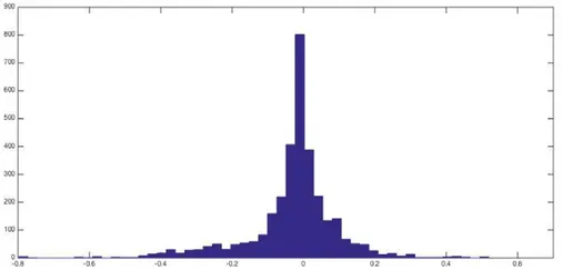
Due to the size, a table for all 5,796 mutual funds, with the previous summary statistics is presented only for a subsample in the appendix. It should allow the reader to grasp the amount of information used in the analysis and the necessity to move from a software to another one in order to speed up the analysis. However, we find that the histogram of the historical returns, Figure 4, can give an immediate and graphical summary of the distribution we are dealing with.

Figure 4: Historical Return Histogram

Given the information set previously analyzed, we will now describe the procedure followed in order to implement the various models used.

We built and test four different models: the traditional Capital Asset Pricing Model as well as the traditional Fama-French-Carhart Model and two modified version of the

(45)

CAPM. The first one introduced a new parameter depending on the square of the market premium as of equation (4); the second one merged the classical version of the CAPM with the Carhart Factor, the Momentum one, as of equation (6).

We decided to estimate time varying betas instead of the classical constant beta. This choice was led by both the willingness to perform a more reliable regression and the decision to build a database for the betas autoregressive analysis model, which will be explained at a later stage. In order to proceed with this kind of estimation, we built a rolling window of 60 months, 5 years as suggested by the literature, used to perform a multi linear regression of the models’ factors over the premium of each fund. Instead of getting only one beta per fund, we got 109 time varying betas for each. The timeframe of the analysis was originally made of 168 months observations, 13 years, which became 109 after the regression, as a consequence of the use of a 60 months window size. The same procedure was used for the alphas estimation. We then proceeded with a detailed comparison and analysis of the outputs. The p-value of each coefficient and the reliability, R^2 and Adjusted R^2, of each single regression were highly taken into consideration: the aim was to understand the forecasting power of each model for the U.S. mutual funds universe, 5796 funds, over the period (2000-2013) analyzed

Again, in order to present the results of the rolling beta we will not use a classical regression representation, as we would have more than 20,000 outputs considering all the results for all the 4 models. Reason why, we calculated the percentage of P-Value

(46)

parameters statistically significant at a 5% level of confidence divided by the total number of parameters estimated in that specific model.

Table 3: Parameters’ P-values percentage significance

Mkt Mkt^2 SMB HML MOM

CAPM 12.68% 83.65%

CAPM^2 12.00% 83.05% 9.72%

CAPM Mom 13.19% 83.62% 34.51% Fama-French-Mom 12.63% 83.40% 42.19% 48.00% 34.50%

The first information that should grab the attention of the reader is the low percentage of significance of the alpha. In all the models the number of the significant alpha is never more than 13.19%: the result does support the absence of persistency in market outperforming for the industry. We can also see that there is no proof of market timing: even if most of the gamma coefficients of equation (4) are positive, less then 10% of them turns out to be statistically significant. Moreover, and maybe surprisingly, the Fama-French factor together with the momentum are not statistically significant in more than half of the parameters estimated suggesting that the market premium might absorbed their explanatory power.

Time Varying Analysis

We estimated an AR (1) on the beta time series obtained with the Rolling CAPM. The choice of keeping only one lag is justified by the monthly frequency of our betas: relevant shocks can be absorbed and processed by the market in that period and, therefore, fund managers can reassess the exposure to the market risk and rebalance their portfolios. In our opinion, it is indeed reasonable to assume that betas, at each time, can be inferred only from the previous period beta, this idea is also supported by the literature discussed.