Woody biomass combustion modeling in moving grate furnaces

(1)

DOCTORAL SCHOOL IN MECHANICAL ENGINEERING XXVI CYCLE

Woody biomass

combustion modeling in

moving grate furnaces

June 2014

Advisor PhD Student

Prof. Giancarlo Chiatti dott. Nello Troccia

PhD School Coordinator Prof. Edoardo Bemporad

(2)

(3)

I

Preface

It is well known that the interest in renewable energy is growing day by day due to different reasons. Some of these are closely related with the present legislation which imposes ever lower emission limits, others are more related with economic features, such as making countries less dependent on fossil fuels. Among the renewable energy sources, biomass plays an important role since it covers about two third of all renewables and it is the fastest growing sector in absolute terms [1]. On this background, in 2009 CRA-Ing (Consiglio per la Ricerca e la Sperimentazione in Agricoltura – Unità di Ricerca per l’Ingegneria Agraria) in cooperation with Roma Tre University launched a project named BTT Project (Bio Thermo Test Project) with the aim of advanced research on biomass utilization for heat and power generation. The project can be roughly divided in three areas: physical and chemical biomass characterization as fuel, biomass combustion characterization in an experimental test bench and biomass combustion simulations. In this thesis the model developed to simulate the biomass combustion process in moving grate furnaces, together with the studies aimed at the elaboration of the model and the obtained results are presented.

The combustion model represents an important tool both for researchers, to better understand how the physical and chemical combustion phenomena depend on the combustion parameters (physical and chemical characteristic of biomass and control parameters of the furnaces), and for the construction companies of furnaces to achieve better design of the combustion system with the aim to meet the emission regulations and to optimize the thermal conversion process inside furnaces.

Working as a unique group together with the CRA-Ing, a large amount of scientific results have been produced, presented and published. The results strictly related with the thesis have been presented at the 20th and 21st European Biomass Conference and Exhibition (Milan 2012 and Copenhagen 2013, respectively) [2] and [3]. Furthermore, in this thesis a literary review on biomass combustion in moving grate furnaces and a work on the study of the sensitivity of thermal conversion processes of biomass on combustion parameters are presented and discussed. In addition to these, there are results that cover other areas of the BTT Project in which I did not participate as a main character and which have been presented, or are going to be presented, in international conferences as well [4] - [8].

(4)

II The topic of biomass utilization for heat and power generation and in particular the simulation of the thermal conversion of biomass in moving grate furnaces is a multidisciplinary theme that involves different scientific disciplines. Some of these disciplines are not the main components of the knowledge of a newly graduate MSc in mechanical engineering. For this reason I took part in two intensive courses on combustion.

The first course took place in September 2012 in Siena (Italy), organised by UIT (Unione Italiana Termofluidodinamica) under the supervision of Prof. G. Croce of the University of Udine. The main object was Computational Thermo-Fluid Dynamics and during the course the thermal heat exchange in compressible and incompressible flows, turbulence and simulation of multiphase flows were presented and discussed.

The second has been organised by CECOST (Centre for Combustion Science and Technology) at Lund University (Sweden) in August 2013. The course (CISS 2013 – Combustion Institute Summer School) had as main objects: Chemical Kinetics by Prof. H. Curran, Turbulent Combustion by Prof. N. Peters and Laser Diagnostic by Prof. M. Aldén.

Moreover, since combustion simulation also deals with numerical problems, a remarkable effort has been made for the discretization and the numerical solution of the partial differential equations system which describes the combustion process. For this reason, I undertook an internship of seven months at Eindhoven University of Technology, working with the Combustion Technology Group headed by Prof. L. P. H. de Goey. During this period, I worked under the supervision of Prof. R. J. M. Bastiaans and Prof J. van Oijen improving the performance of the simulation program and making it more reliable and efficient.

Acknowledgments

During this scientific trip I have been supported by a large number of people. Here I would like to thank some of them. First of all, I would like to thank my advisor Prof. G. Chiatti. Three years ago he gave me the opportunity to cooperate with his group in this project. During this period, he supported and advised me, reviewing my work continuously. Nowadays I can say that this chance changed my life completely giving to me the opportunity to grow as a man and under a professional point of view. I would like to thank Ing. F. Gallucci and Dott. L. Pari of the CRA research centre. They managed and they are still managing at best one of the most advanced projects on renewable energy conducted in Italy. Thank you to PhD. F. Palmieri for the support given during the initial phase of my PhD studies, when I started to deal with biomass combustion. Thank you to Ing. M. Amalfi, we worked together for three years sharing difficulties and nice moments. It will be difficult to forget this scientific and, first of all, life experience with him.

I would like to thank you Prof. L. P. H. de Goey, Prof. R. J. M. Bastiaans and Prof J. van Oijen that gave me the opportunity to work with The Combustion Technology Group at the Technology University of Eindhoven, improving the performance of my model. Thank you to all the PhD

(5)

III students and postdocs of Combustion Technology Group, in a particular way to MSc U. M. Goktolga, and PhD A. Donini.

Finally, I would like to think of the people which are part of my life. My parents, Alessandro and Vilma and my sisters Francesca and Marta together with my grandmother Teresa and my uncle Maurizio. You are my family and you always supported me in my decision, thanks a lot for this. All my friends of the “Saturday Night Group”, we grew together and together with you I spent the most beautiful moments of my life. Thank you friends!. Thank you to PhD C. De Luca. Once I met you in Siena, you became my close friend and technical confidant. Thanks to your support I overcame the most difficult moments of my PhD studies. The last thank you to Stéphanie. You became part of my life while I was in Eindhoven, making my period abroad one of the most adventurous experiences in my life.

Rome, April 2014. Nello Troccia

(6)

i

Index of the figures

A TYPICAL OUTLINE OF A BURNING BIOMASS BED. ... 8 FIGURE 1

SCHEMATIC REPRESENTATION OF A BIOMASS COMBUSTION MODEL. ...10 FIGURE 2

CALCULATION DOMAIN DISCRETIZATION. ...24 FIGURE 3

TANK-AND-TUBE SCHEME. ...25 FIGURE 4

SCHEMATIC REPRESENTATION OF THE TEST RIG OF KLEAA [57]. ...29 FIGURE 5

COMPARISON BETWEEN EXPERIMENTAL AND CALCULATED BED TEMPERATURES PROFILES. THE FIGURE 6

VALUES IN THE LEGEND STAND FOR DISTANCES FROM THE GRATE...31 BIOMASS BED: FROM SPATIAL TO TIME COORDINATE. ...32 FIGURE 7

SOLID PHASE TEMPERATURE CONTOUR IN SIMULATION 1. ...35 FIGURE 8

SOLID PHASE MOISTURE MASS FRACTION CONTOUR IN SIMULATION 1. ...37 FIGURE 10

SOLID PHASE VOLATILE MASS FRACTION CONTOUR IN SIMULATION 1. ...38 FIGURE 12

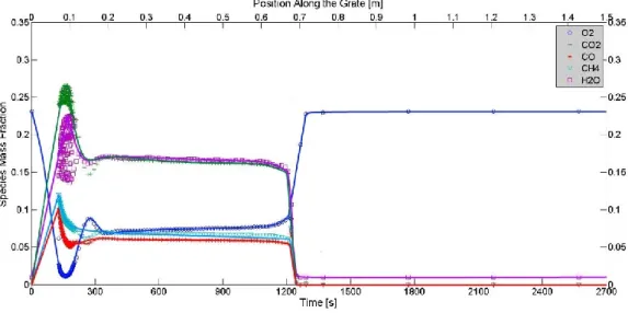
SOLID PHASE VOLATILE MASS FRACTION AT DIFFERENT HEIGHTS FROM THE GRATE IN FIGURE 14

SIMULATION 1. ...39

SOLID PHASE CHAR MASS FRACTION CONTOUR IN SIMULATION 1. ...40 FIGURE 16

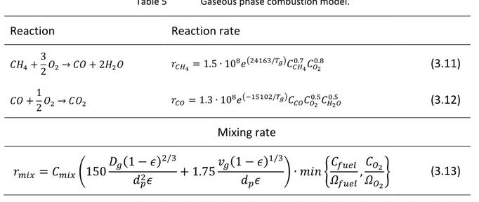
GAS FLOW RATE ABOVE THE BED SURFACE IN SIMULATION 1. ...42 FIGURE 18

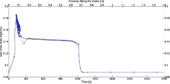
GASEOUS SPECIES MASS FRACTION ABOVE THE BED IN SIMULATION 1. ...43 FIGURE 20

(10)

v SOLID PHASE TEMPERATURE CONTOUR IN SIMULATION 2. ...45 FIGURE 24

MIXING MODELS: A) NO-MIXING; B) LAYER-OVERFED; C) LAYER-EXCHANGED. ...75 FIGURE 50

SINUSOIDAL MIXING PATTERN. ... ERRORE. IL SEGNALIBRO NON È DEFINITO. FIGURE 51

SCHEMATIC REPRESENTATION OF THE EXPERIMENTAL FACILITY BY ZHOU ET AL [34]. ...79 FIGURE 52

PROBES POSITION IN THE EXPERIMENTS OF FREY ET AL [61]. ...83 FIGURE 53

MAIN MENU OF THE PROGRAM. ...85 FIGURE 54

SOLVER PARAMETERS. ...86 FIGURE 55

(11)

vi PROCESS SWITCHES AND BOOLEANS (A PARTIAL REPRESENTATION). ...87 FIGURE 56

PROCESS PARAMETER (SUB-SECTION OF PROCESS CONSTANT). ...88 FIGURE 57

FLOW CHART OF THE BRAIN SUB-ROUTINE. ...89 FIGURE 58

FLOW CHART OF THE HEART SUB-ROUTINE. ...91 FIGURE 59

(12)

vii

Index of the tables

MOISTURE EVAPORATION RATE [KG/M3S]...12 TABLE 1

DIMENSIONLESS NUMBER FOR CONVECTIVE MASS AND HEAT TRANSFER...13 TABLE 2

DEVOLATILIZATION REACTION MODELS. ...14 TABLE 3

DEVOLATILIZATION MODEL. ...15 TABLE 4

GASEOUS PHASE COMBUSTION MODEL. ...16 TABLE 5

CHAR OXIDATION REACTION. ...17 TABLE 6

ULTIMATE ANALYSIS OF THE WOOD (MASS FRACTION ON DRY BASIS). ...30 TABLE 7

EXPERIMENTAL CONDITIONS. ...30 TABLE 8

SIMULATION SETTINGS FOR THE REFERENCE CASE. ...34 TABLE 9

SIMULATION SETTINGS ...34 TABLE 10

RADIATION INTENSITIES FOR THE TWO FLUX MODEL [W/M2]. ...61

TABLE 11

TWO FLUX MODEL ASSUMPTION. ...61 TABLE 12

THERMAL CONDUCTIVITY [W/M2K]. ...61 TABLE 13

BEER’S LAW MODEL FOR RADIATIVE HEAT EXCHANGE. ...62 TABLE 14

CONVECTIVE HEAT TRANSFER COEFFICIENT. ...63 TABLE 15

MOISTURE EVAPORATION RATES [KG/M3S]. ...64 TABLE 16

CONVECTIVE MASS TRANSFER COEFFICIENT. ...64 TABLE 17

DEVOLATILIZATION RATES BY SHIN AND CHOI [23]. ...65 TABLE 18

DEVOLATILIZATION RATES BY YANG ET AL [29]. ...65 TABLE 19

DEVOLATILIZATION RATES. ...66 TABLE 20

VOLATILE COMPOSITION (PERCENTAGE ON VOLATILE MASS). ...66 TABLE 21

TAR FORMULA. ...67 TABLE 22

TAR REACTION RATE [MOL/M3S]. ...67 TABLE 23

HOMOGENEOUS REACTION RATES. ...68 TABLE 24

RC RATIO OF CO/CO2 FORMATION RATE. ...70 TABLE 25

(13)

viii CHAR COMBUSTION RATE. ...70 TABLE 26

MASS TRANSFER COEFFICIENT FOR CHAR COMBUSTION REACTION. ...71 TABLE 27

CHAR COMBUSTION RATE BY ASTHANA ET AL [35]. ...71 TABLE 28

SHRINKAGE VOLUME MODEL. ...73 TABLE 29

SPECIFIC HEAT OF GASEOUS AND SOLID SPECIES. ...77 TABLE 30

PROPERTIES OF WOOD [55]. ...78 TABLE 31

EXPERIMENTAL SETUPS FOR DIFFERENT AUTHORS. ...80 TABLE 32

(14)

2

1. Introduction

1.1. Background

The control of greenhouse gas emissions, responsible for climate changes, is a problem that needs global solutions. Indeed, emissions have no boundaries and cause global effects irrespective of the geographical location of the emitting source. For this reason, the European Union (EU) has introduced a new strategy concerning the renewable sources, energy efficiency and the greenhouse gas emissions, eliminating, at least on a political level, the boundaries among the policies on climate changes and the energetic policies.

The new European strategy is named “20 20 20” [9] and establishes three ambitious targets to achieve by 2020:

 A 20% reduction in EU greenhouse gas emissions from 1990 levels;

 Raising the share of EU energy consumption produced from renewable resources to 20%;

 A 20% improvement in the EU's energy efficiency.

The operative implementation of this strategy is the Climate–Energy Package. This package contains all the main instruments through which EU intends to achieve its targets on greenhouse emissions reduction, energy efficiency and renewable energy sources.

In addition to this, it is of non-minor importance that the production of oil is concentrated in a limited number of countries. This scenario drives the interest of countries with small fossil fuel reserves on the valorisation of renewable energy sources.

In this context biomass energy sources represent an important opportunity. Indeed, they are a complex form of solar energy accumulation and if they are produced, processed and used with efficient and sustainable methods, they represent a key renewable energy source.

The term biomass includes a wide collection of substances (e.g. energy crops, residues of agricultural and forestry activities, municipal waste, etc.). Furthermore, energy use of biomass can be obtained by direct combustion or through its conversion in solid, liquid or gaseous fuel. This study considers only woody biomass from energy crops or as residues of agricultural and forestry activities and its direct thermal conversion as fuel in moving grate furnaces. Indeed,

(15)

3 this technology is the most utilized, from small scale for civil applications to large scale for industrial applications. The advantages of the latter, in respect to fluidized bed furnaces or pulverized fuel furnaces, are: the minor pre-treatment of fuel, lower installation and management costs and better knowledge of technology.

As always, there are advantages and disadvantages in the utilization of biomass as renewable energy source. Differently from wind and solar energy, biomass can be stored in a less expensive way [4] - [5] and it is less sensitive to the temporary change in the meteorological conditions. Moreover, it can be used in existing plants originally developed for fossil fuels with minimal or no modifications. This is the case, for instance, of the grate furnaces deigned for coal combustion.

The main technical disadvantage is related with sustainable production and supply. A huge amount of effort is done to improve the recovery and the harvesting techniques [10] - [12] and to solve the problems related with biomass logistics [13] - [14]. The other disadvantage has more social implications and is related with the increase of the cost of food due to the competition for land and water between biomass energy crops and crops for food supply. This global scenario attracts the interest of numerous research institutions and universities committed in scientific projects on different aspects of the same problem: make the energy biomass utilization more sustainable, affordable and accessible.

1.2. Aim of the project

During the combustion process in grate furnaces not only the thermal conversion of biomass into energy, but also the formation of pollutants occurs. Thus, it is readily apparent that a detailed understanding of the occurring phenomena is central to define the right strategies for controlling and optimizing the combustion process.

With these intentions, it is possible and interesting to investigate biomass combustion via experiments. Observation on full-scale furnaces operation can show temperature distribution over the solid bed and flue gas composition via probing and or laser techniques. Unfortunately, in most cases full scale experiments are prohibitively expensive and the alternatives are laboratory-scale experiments. The resulting information must be extrapolated to full scale and this is not always a simple and reliable task. The problem can be solved with the use of numerical calculations which guarantee features such as low cost and high speed also in case of parametrical investigation.

Since biomass combustion in moving grate can be roughly divided in two stages, the heterogeneous in-bed combustion stage and the over chamber gaseous phase combustion, to achieve the goal of flexible controlling strategies, the development of a packed bed combustion simulation model is of primary importance. The aim of the thesis is the formulation of a model able to simulate the combustion process in a fuel packed bed. The outputs of the model are organised in terms of temperature, gaseous species concentration and gas flow rate profiles at the boundary layer between the solid fuel and the over bed combustion chamber. These results

(16)

4 can be used as input in a CFD model of the grate furnace to simulate the gaseous combustion outside the fuel bed layer and to obtain comprehensive results on biomass combustion.

1.3. Outline

Chapter 2 consists of a brief overview on biomass combustion systems. The three main technologies available are presented with focus on grate furnaces. The combustion process of biomass is described in detail and advantages of modeling are explained.

In Chapter 3 the mathematical relations chosen to model the physical and chemical phenomena that occur during biomass combustion are presented and critically discussed. In Chapter 4 the continuity equations, that describe the system’s behaviour, and the discretization and solution method applied to solve the PDE’s are introduced.

In Chapter 5 the validation of the developed simulation code is performed against experimental results reported in literature by other authors.

In Chapter 6 the results of the six simulations performed with the aim of understanding the influence of the biomass characteristic and operational conditions on the thermal conversion of biomass are presented and discussed.

(17)

5

2. Biomass utilization for power generation

The energy use of biomass can be obtained by direct combustion or through its conversion in solid, liquid or gaseous fuel. In this chapter the current technologies available for direct conversion of biomass will be introduced with particular regards to the thermal conversion in grate furnaces.

2.1.Biomass combustion systems

Biomass energy conversion via combustion has the advantage to rely on well-developed technologies of heterogeneous burners like coal furnaces, which are the foundation of energy power generation around the world. Biomass combustion technologies show also, especially for large-scale applications, similarities to waste combustion systems, but since biomass fuels are utilized, the necessary flue gas cleaning technologies are less complex and therefore cheaper. Generally speaking coal plants could be inexpensively retrofitted to burn biomass, MSW or a blend of these products in a process called co-firing.

However traditional technologies have shown difficulties on burning inhomogeneous fuels, like poor power regulation and problems concerning emissions. It is necessary to develop new furnace systems to burn biomass in an efficient, cheap and clean way. Biomass burning systems are still affected by those penalties which require further investigation and developing to solve these problems .

Industrial furnaces usually utilize electronic air supply regulation and oleo-dynamic fuel feeding systems. The combustion technologies may be distinguished in three categories: fixed bed, fluidized bed and pulverized bed. In fixed bed systems, which concern grate furnaces and underfeed or cigarette stokers, primary air flows through a porous fixed bed where drying, devolatilization and solid combustion take place. Secondary air is fed upside the bed to complete reactions and limit emissions with staging air techniques.

Fluidized bed furnaces utilize a mixture of fuel and an inert material like sand which flows through nozzles in the combustion chamber. Fuel feeding may be operated at different velocities, making it possible to distinguish between bubbling fluidized beds (BFB) and circulating fluidized beds (CFB).

(18)

6 Pulverized fuel systems use fuel reduced in small particles as it can be fed to the furnace with the primary air supply. Char combustion and gas burnout are achieved without secondary air injection.

2.1.1. Grate furnaces

Grate furnaces can be divided into fixed grates, moving grates, travelling grates, rotating grates and vibrating grates. These systems have different performances in relation to the fuel burnt. Grate furnaces are well suited to biomass with a high moisture ratio, different particle sizes and high ash content, so they can be fed with blends. To cope with non woody biomass such as straw or grass it is necessary to utilize special grate constructions like rotating or vibrating grates. This is needed due to differences in combustion behavior and ash melting point between woody and non woody biomass. A good system should work with homogenous fuel and air distribution along the grate. This is the best condition to limit fly ashes and high excess air ratios. As can be seen in experimental work done by Amalfi [15], fuel feeding and grate movement has to be smooth to avoid CO and organic compounds release in flue gases.

Grate systems usually employ air staging also along the grate, this with the purpose of supplying the specific amount of air to the different zones where drying, pyrolysis and char combustion occur. Air staging along the grate also allows partial load operation and correct combustion with different fuels. The reliability of the grate mechanism can be improved with water cooling to limit slagging on surfaces. In grate furnaces, it is of crucial importance how secondary air mixes with bed gases. This because primary chambers lack the turbulence necessary for a proper mixing and thus a good homogenous combustion. A better mixing means less air excess ratio, thus higher thermal efficiency of the burner. The geometry of these systems may be counter, co-current or cross flow operations in relation to how fuel and flue gas flow in respect to each other.

Counter flow systems are well suited to fuels with high moisture content and low heating value. The flame passing above fresh fuels permits fast drying and good water vapor evacuation from the chamber. Co-current flow chambers increase residence time of both fuel and gases in the furnace which may lead to a better combustion at low air ratio which directly reflects on NOx and unburned emission reductions. This geometry is usually used with straw based fuels and preheated air supply. Cross-flow systems are a combination of the first two geometries.

2.1.2. Fluidized bed furnaces

FBC systems have been operating since 1960 for the burning of industrial waste. They consist of vertical vessels where air injection is performed on the bottom trough a perforated plate and bed material is mixed with silica or dolomite while being suspended by air flow. They perform intense heat transfer and good mixing which allow a good combustion even with low excess air ratio. They suffer from ash sintering in the bed so it is necessary to limit the temperature of the chamber to 650-900 °C by internal heat exchangers, EGR or water injection. Due to good mixing abilities, FBC systems can also burn various fuel mixtures, however these systems are

(19)

7 limited by fuel particle size and impurity content. Particle sizes below 40mm and fuel pretreatment are recommended. Regarding emissions they perform well on NOx CO flue gas fractions due to good mixing and effective air staging with low excess ratio, it is also possible to use additives like limestone to trap S, but they suffer from inert dust entrained on flue gas which require massive and efficient dust separators before the chimney. FBC furnaces are expensive and therefore interesting only for large scale applications of above 20 MWth.

2.1.3. Pulverized bed furnaces

In these furnaces fuel, in the form of sawdust, is pneumatically injected in the chamber, using primary air as fuel vector. This kind of burners require carefully controlled operation of the fuel injector and fuel preparation to ensure stable working conditions. Indeed small fuel particles exhibit concurrent devolatilization and char combustion in an explosion-like reaction. Usually injectors fire the chamber tangentially to assure rotational flows and flue gas recirculation as turbine burner scheme .This mechanism permits rapid load changes and low excess air ratio but cause high energy density levels on the chamber which requires water cooling. Muffle dust furnaces are commercially available in the size 2-8 MWth. They offer good emission control due to good mixing and air staging but high flue gas velocities determine issues like walls erosion and bottom ash carriage in flue gas.

2.2. Biomass combustion in grate furnaces

The process of biomass combustion involves a series of physical and chemical phenomena strictly coupled with each other. Under a technological point of view, there are different solutions for biomass combustion: from simple fixed bed applications to the high complexity pulverized bed power plants. Anyway, irrespective of the complexity of the combustion technology and fuel characteristics, the combustion process can be divided into several general phenomena: initial heating, moisture evaporation, devolatilization of volatile matter and char formation, heterogeneous and homogeneous reactions and particles shrinkage [1]. While these phenomena proceed, the gases flowing through the packed bed and the biomass particles exchange heat and mass between each other. With regard to the grate furnaces, the overall combustion process can either be a continuous or a batch process, and air addition can be carried out either by forced or natural draught. Batch combustion is used in some small-scale combustion units, some of which also use natural draught. This is typical for traditional wood-stoves. Medium to large-scale combustion units are always continuous combustion applications, with forced draught [16].

Physical and chemical phenomena previously introduced are strictly connected to the temperature of the fuel and, as shown in Figure 1, it is possible to identify a reaction front which moves downwards through the fuel bed.

(20)

8

A typical outline of a burning biomass bed. Figure 1

When the fuel enters the combustion chamber, the radiative heat power coming from the flames and the walls of the furnaces heats up the bed of biomass and the evaporation process can start. Since drying uses the energy released from fuel combustion for water evaporation, during this process the temperature of the biomass remains around 100 °C. This means that evaporation of moisture lowers the temperature in the combustion chamber and slows down the combustion process. In wood-fired boilers, for instance, it has been found that the combustion process cannot be maintained if the wood moisture content exceeds 60 % on a wet basis. The wet wood requires so much energy to evaporate contained moisture, and subsequently to heat the water vapour, that temperatures are reduced below the minimum temperature required to sustain combustion. Consequently, moisture content is a very important fuel variable that influences the combustion process [16]. Once the evaporation is ended the temperature of the solid bed can increase again and the devolatilization process can take place. The devolatilization of volatile matter can be defined as thermal degradation of the virgin biomass and during this process the fuel is decomposed, due to the rise of temperature, into three main products: gas, tar and char. The numerous studies concerning this process, that can be found in literature, show that the devolatilization of volatile matter is a combination of successive endothermic and exothermic reactions. However, the explanations of the biomass’ behavior during the degradation differ significantly through the different authors. Park et al [17] justify the temperature behavior of biomass particles considering the formation of a new solid phase named “intermediate solid” from virgin biomass through an endothermic reaction, which degrades into char with an exothermic reaction. Bilbao et al [18] presumed that the first endothermic reaction is due to the cellulose and hemicellulose decomposition, whereas lignin decomposition accounts for the second exothermic reaction. Also Di Blasi et al [19] explain the exothermal process with lignin decomposition while the endothermic process is attributed to

(21)

9 the holocellulose and extractives decomposition. Instead, Gronli et al [20] attributed the exothermic behavior of wood pyrolysis to the tar cracking reaction. The gases released by the biomass are mainly composed of H2O, CO, CO2, CH4 and H2, whose mass fractions depend on the heating condition (heating rate and temperature value) and the chemical composition of the virgin biomass. For engineering applications, a constant composition of the released gases is usually assumed [34], [39] and [50]. As well as gases also tar (condensable fraction of volatile matter) is released during devolatilization. The gases released during the thermal conversion of the biomass can react among each other resulting in new species or they can oxidize with oxygen present in the air supplied from under the grate. The oxidation of the gases starts inside the solid bed and is completed in the combustion chamber above the solid layer by supplying secondary air. When the devolatilization of volatile matter is completed the bed is mainly composed of char. The reaction of the char with oxygen (heterogeneous reactions) gives as product CO (gasification) and CO2 (complete combustion). The fraction of CO and CO2 produced during char combustion depends mostly on the combustion temperature but also on the air excess. The gasification of char can occur also with water vapour resulting in H2 and CO. During this phase the bed temperature reaches the maximum value (approximately 1200 °C) and once the char combustion has taken place only ash is left on the grate. In the last part of the grate the ash formed by the char combustion is cooled by the air supplied from under the grate. As said at the beginning of the paragraph, the phenomena described are typical of the biomass combustion process and their occurrence does not depend on the combustion system technology and the fuel characteristics. Anyway, the physical and chemical properties of the fuel such as biomass particles dimension, moisture content, low heating value and chemical composition; and the operational variables of the combustion system such as primary and secondary air flow rate and the grate movement have a relevant influence on the duration of each phenomenon and the temperature values reached during the global combustion process. Thus, these parameters have a significant impact on the overall efficiency of the thermal conversion system.

2.3. Modelling biomass combustion

Due to the considerable variations in the quality of the biomass fuel that can be used in biomass power plants, one of the main aims of the studies in biomass combustion is to gain wider knowledge on what happens when biomass is burned and, in particular, what changes occur when the fuel characteristics and the operational variables of the conversion system vary. Modelling, together with experiments, enables a cost-effective approach for future biomass combustion application design, and can improve the competitiveness of biomass combustion for heat and electricity generation. Modelling improves our understanding of the fundamental processes involved in biomass combustion, and may significantly reduce the “trial and error” development time needed if experiments only are used for design optimization. Parametric studies can be carried out that reveal the relative influence of different combustion process variables on emission levels and energy efficiency. This enables us to make the correct

(22)

10 decisions with respect to the optimal design and operational principles of the biomass combustion applications.

Combustion in grate furnaces occurs in two distinct regions: the solid bed region, where the combustion process takes place within the fuel bed that is travelling on the grate and the freeboard region, where the volatiles emitted from the bed surface undergo combustion reactions. Thus, as shown in Figure 2, a complete biomass combustion model is always composed of two parts: the model which simulates the combustion of the solid phase on the grate, coupled with a Computational Fluid Dynamics (CFD) model of the gaseous phase combustion in the chamber above the solid bed. The outcome of the first one, in terms of gas temperature, composition and flow rate, represent the inlet data for the CFD model. At the same time, the results by the CFD in terms of gas temperature represent an input for the biomass bed model.

Schematic representation of a biomass combustion model. Figure 2

(23)

11

3. Biomass combustion phenomena

3.1. Introduction

During the last two decades, mathematical models of biomass combustion have been developed by many authors: Shin and Choi [23] have developed a one dimensional transient model of waste incineration in moving grate furnace, van der Lans et al [24] have presented a two dimensional model of straw combustion in a cross current moving bed, Goh et al [25] have developed a mathematical model for combustion of solid waste in a travelling grate incineration based on an unsteady-state static bed model. Yang et al [26] - [33] have conducted different studies regarding combustion of biomass material, from the influence of the fuel properties to the influence of the physical and chemical phenomena occurring during biomass combustion, considering municipal solid waste as well as straw and other kind of biomass fuels. Zhou et al [34] have developed a one dimensional transient model of straw combustion, Johansson et al [35] have conducted an analysis of the uncertainty of model parameters related to heat transport, reaction rates and composition of volatiles, Albrecht et al [36] have introduced a new modelling approach for biomass furnaces using a flamelet model for the prediction of combustion and NOx emission in a pilot-scale low-NOx biomass grate furnace, van Kuijk et al [37] and [38] have developed a sub-model to simulate reverse combustion, Asthana et al [39] have proposed a steady-state two dimensional model to simulate on-grate municipal solid waste incineration, Boriouchkine et al [40] have developed a one dimensional transient model to study the effect of operation parameters on biomass firing, Miljkovic et al [41] have proposed a two dimensional approach for straw combustion modelling in moving grate furnaces and Martinez and Nussbaumer[42] have developed a one dimensional transient model of biomass combustion with combustion optimization purposes.

3.2. Physical and chemical models

During the biomass combustion process a series of physical, chemical and thermal phenomena occur. As previously reported in paragraph 0, these phenomena are: initial heating, moisture evaporation, devolatilization of volatile matter and char formation, heterogeneous and homogeneous reactions and bed shrinkage. Thus, the development of a model that simulates the biomass thermal conversion requires the description, through mathematical relations, of

(24)

12 each mentioned phenomena. In this chapter, the mathematical models used by different authors are introduced and discussed in order to show the various possibilities of the phenomena modelling and define which are suitable for an implementation in our model.

3.2.1. Moisture evaporation

Woody biomass used in industrial furnaces presents an amount of moisture which can vary between 5 % and 50 % on dry basis [31]; depending on the biomass type, pre-treatment (e.g. drying) as well as storage time and mode. The drying of porous media, such as a wood chips bed, is a complex process involving heat and mass transfer phenomena and it was studied in detail by several authors e.g. Kowalski [43], Younsi et al [44] and Di Blasi [45]. In a saturated wood particle, water is bounded in the porous structure in three ways: chemical bounded water, physical-chemical bounded water and physical-mechanical bounded water. The first one does not participate to the drying process because too much energy is required to break the chemical bounds; the second one is enclosed in the organic material of plants and is also referred to as adsorptive water and the last one is the free water that fills the pores of the wood. The free water leaves the biomass first because its evaporation process is less energy demanding than adsorptive water. Moisture evaporation from biomass particles can be modelled using three main different models:

 Diffusion limited model;  Radiative model;

 Arrhenius law model.

The third method is applied by Di Blasi et al [46] to describe moisture evaporation kinetics in updraft gasifiers to reduce the complication in numerical calculation, and this is done as well by Boriouchkine et al [40] and Johansson et al [35] in their biomass combustion models. The second method is used in coupling with the first as in the work of Goh et al [25] and Yang et al [29] - [33]. In these works when the biomass temperature is under 273 K the evaporation mechanism is diffusion limited and when the temperature is over 273 K the mechanism is radiative. In this situation all the heat is used to dry the biomass fuel. Other authors, such as Shin and Choi [23], Zhou et al [34] and Asthana et al [39] prefer to use a diffusion limited model only. The relations used to describe each model are listed in Table 1.

Moisture evaporation rate [kg/m3s]. Table 1

Diffusion limited model ( ) (3.1) Radiative model [ ( ) ( )]

(3.2)

(25)

13 Where S is the specific surface area per volume of solid matter, ε the emissivity of the grey body, Tg and Ts the gaseous and solid phase temperature, respectively. Tw the temperature of

the walls of the combustion chamber, the Stefan-Boltzmann constant, Hevap the latent heat of

water evaporation, and the frequency factor and the activation energy of the Arrhenius law, R the universal gas constant, ρs the mass density of the solid phase, XH2O the

mass fraction of moisture in the solid phase, Cws and Cwg the water vapour mass concentrations

on the particle surface and in the gaseous phase, respectively. The value of Cws is assumed to be

equal to the water vapour concentration in the saturation conditions at the temperature of the solid particle. The mass transfer coefficient hm and the convective heat transfer coefficient ht

are determined using the relations reported for a packed bed of spherical particles by Wakao and Kaguei [47] (see Table 2).

Dimensionless number for convective mass and heat transfer. Table 2

Sherwood Number (3.4) Nusselt Number (3.5)

Where Re, Sc and Pr are the dimensionless number of Reynolds, Schmidt and Prandtl, respectively.

Since we are at an early development of our code, the less computational demanding Arrhenius model by Di Blasi et al [46] has been implemented. This decision does not preclude any further development of the code with the implementation of more detailed and computational demanding models such as the diffusion-radiative model.

3.2.2. Devolatilization of volatile matter

When subjected to external heating, solid fuels start to decompose, giving a mixture of volatile species and solid carbonaceous residual products. The products of this thermal degradation process are usually grouped into a few main components. Each component represents a sum of numerous species which are lumped together to simplify the schematization. Generally, the product groups considered are: gas, tar and char [21]. Char is the carbon-rich non-volatile residue. Tars are any several high molecular weight products that are volatile at the devolatilization temperature but condense near room temperature. Gases include all lower molecular weight products (e.g. CO, CO2 and CH4).

As reported by Di Blasi [21], kinetic models of biomass devolatilization can be classified into three main groups:

 One-step global models;

 One-stage, multi-reaction models;  Two-stage, semi-global models.

(26)

14 A simple way to represent the reactions of these three main groups is reported in Table 3. In the one-step global models a one-step reaction is used to describe degradation of the solid fuel. An Arrhenius law is used to describe the temperature dependence of the weight loss of the fuel. The one-stage multi reaction models use one-stage kinetics models but describe the degradation of the solid to char and several gaseous species. The two-stage models include both primary reactions of virgin solid degradation and secondary reactions of evolved degradation products. In addition to these, in literature it is possible to find more complicated models, such as those proposed by Park et al [17] and Grieco and Baldi [48], used to explain the thermal behavior of the fuel particle during the thermal degradation or the competing parallel reaction model originally proposed by Shafizadeh and Chin [49]. In conclusion it is relevant to note, as reported by Di Blasi [21], that kinetic data about devolatilization of biomass varies considerably due to the different set up and techniques of experiments (e.g. heating rate, direction of heat flux, temperature and pressure) as well as physical and chemical properties of biomass (e.g. particle size, moisture content, chemical composition). This means that values of kinetic parameters are not representative of the true physic-chemical process governing the degradation of solid fuels but are valid only for correlating experimental data.

Devolatilization reaction models. Table 3

Reaction Model Reaction Scheme

One-step global model _→ (3.6)

One-stage, multi-reaction model _→ (3.7)

Primary reactions Secondary reactions

Two-stage, semi-global model

→

→ (3.8)

→ →

In the works related with the biomass combustion modeling, since the main aim is not only the description of the thermal degradation of the biomass due to the devolatilization but the overall combustion process, the models used to describe the devolatilization are simple one-step global models [24], [29] - [31], [33] - [35], [39] - [42].

(27)

15 This means that the devolatilization rate is proportional to the remaining mass of the volatile in the solid phase through the rate constant defined by an Arrhenius law (see Table 4).

Devolatilization model. Table 4

Devolatilization rate (3.9) Devolatilization rate constant ( ⁄ ) (3.10)

Where is the mass fraction of volatile in the solid phase, and the frequency factor and the activation energy for the devolatilization process. In our model, the parameters reported by Yang et al [29] for slow case were used.

Regarding the composition of the volatiles released due to the biomass decomposition, different approaches can be found in literature. Yang et al [33], Zhou et al [34], Asthana et al [39] and Di Blasi [50] apply a decomposition of the volatiles in different species using constant values; Shin and Choi [23] and Yang et al [29] consider the volatile as a unique species CnHmOl. In this work we follow the approach of Asthana et al [39] considering a decomposition of the volatile in different species using constant values which meet the elemental composition, the proximate analysis and the calorific value of the woody biomass fuel considered.

3.2.3. Homogeneous reactions

Volatile species, released during biomass devolatilization, react inside the packed bed with each other, with the oxygen supplied from the bottom and with the carbonaceous solid residue of the solid fuel. In literature, different approaches are developed to simulate the gaseous phase combustion inside the packed bed. Van der Lans et al [24] assume that only char reacts with O2 inside the bed, instead Shin and Choi [23] consider the generic hydrocarbon CxHy to be the only product of the devolatilization and assume that it is first partially oxidized to CO and then further converted to CO2. Yang et al [29] - [31] uses the same scheme of Shin and Choi but they also take into account the production of the species H2 from the CxHy reaction with O2. Moreover, they consider that gaseous species first have to mix with surrounding air before their combustion can take place. For this reason they introduce a mixing rate proportional to the energy loss through the bed and define the actual reaction rates of volatile species as the minimum of the kinetic rates and the mixing rates with the oxygen. Also Zhou et al [34] take into account that the volatile combustion is not only controlled by kinetic rates but also by the mixing rates of the gases with the primary air flow, but they differentiate the volatiles species in CO, CO2, CH4, CnHm, H2 and tar. The tar is modeled as the hydrocarbon CH1.84O0.96 with a molecular weight equal to 95 and gives as combustion products CO and H2O.

In our model we follow the scheme of Asthana et al [39] considering as gaseous species CO, CO2, CH4, H2O. In addition, we consider that the gases released during devolatilization first

(28)

16 have to mix with the air stream provided from under the grate. For this reason, we introduce a mixing rate as defined by Johansson et al [35].The complete scheme of the reactions is reported in Table 5.

Gaseous phase combustion model. Table 5

Reaction Reaction rate

→ ( ) (3.11) → ( ) (3.12) Mixing rate ( ( ) ( ) ) , - (3.13)

Where Ci are the molar concentrations of gaseous species expressed in [mol/m3], Cmix is an

empirical constant (usually equal to 0.65) and Ω the stoichiometric coefficient in the chemical reaction.

3.2.4. Heterogeneous reactions

Heterogeneous reactions involve the combustion/gasification of the char remaining after devolatilization with the oxygen and the other gaseous species present in the gaseous phase flowing through the bed. The overall rates that control these reactions are given by the combination of the chemical reaction rates and the mass diffusion rates of the gaseous species toward the surface of the solid fuel, where the reactions take place. The primary products of char combustion are CO and CO2. Final burnout of CO takes place in the gaseous phase.The appropriate stoichiometric coefficient for oxidation of char is not readily apparent and it is necessary to define the term , that depends on the ratio of CO/CO2 formation rate. In

(29)

17

Char oxidation reaction. Table 6

Reaction → ( ) ( ) (3.14)

Stoichiometric ratio ( ⁄ ) ( ⁄ ⁄ ⁄ ) (3.15)

CO/CO2 ratio ⁄ ( ) (3.16)

Reaction rate (3.17)

Specific bed surface ( ) (3.18)

Surface reduction coefficient

(3.19)

Overall rate constant ( )

(3.20)

Chemical rate constant ( ⁄ ) _(3.21)

Mass transfer coefficient

( ) (3.22)

Where is the active surface reduction coefficient, k0 the overall rate constant of char

combustion/gasification, kc and hm the chemical rate constant of char combustion/gasification

and the mass transfer coefficient of oxygen toward the reaction surface.

The scheme model implemented is common to different authors [24], [29], [31], [33], [34], [41] and [42] and it has been chosen since it takes into account both chemical and diffusional rate constants for char combustion. The active surface reduction coefficient is taken from the work of Asthana et al [39] and the mass transfer coefficient hm is defined as reported by van der

Lans et al [24].

In this work, no char reaction with gaseous species different from oxygen is considered. This decision does not preclude a further development of the code with the implementation of more detailed models such as implemented by Johansson et al [35], Asthana et al [39] and Boriouchkine [40], which consider also the gasification of char with water steam, H2 and CO2.

3.3. Volume change of bed during combustion

The reduction of the bed volume during the combustion process is related with the mass loss due to drying, devolatilization and char combustion. The volume shrinkage does not have the same magnitude during the different phases of the combustion process. For this reason, as a first approximation it can be considered that the mass released during drying and

(30)

18 devolatilization is replaced by internal porosity and no bed volume reduction occurs during these phases [39] and [42]. The change in bed height is then associated only with the char consumption.

The relation proposed to model this phenomena is reported below.

(

) ( )

(3.23)

Where is the mass of char burned per unit volume of bed, the mass of char per unit volume of bed and is the volume occupied by the ash. The subscripts 0 refers to the initial conditions.

(31)

19

4. Governing equations of the biomass combustion model

In this chapter, the governing equations of a 1-D transient model for biomass combustion in moving grate furnaces are introduced. To describe physical, chemical and thermal behaviour of biomass beds the following assumption are made:

 biomass particles are schematized as spherical particles[23], [29] - [31], [35] - [40] and [42];

 thermal gradients inside the particle are neglected [31] (packed bed is described as formed of two homogeneous phase: gaseous and solid phase);

 the gaseous phase is described as an ideal gas[34] and [40];

 the pressure of the gaseous phase through the bed is constant and equal to the atmospheric pressure [23] and [29] - [40];

 the gaseous species considered in the simulation are CO, CO2, H2O, O2, H2, CH4, and inert gas N2 [23], [29] and [31];

 heat produced in char combustion is accounted in the solid phase [40];

 temperature of the gas released from the solid is the same of the solid phase [40]. The bed behavior can be modeled as a 1-D transient phenomenon since the gradients, such as temperature and chemical species concentration gradients, in the direction of the movement of the grate are negligible compared to those in the direction of the gas flow. Then, heat and mass transfer in the direction of the bed movement can be ignored [23], [34], [37], [38], [40] and [42].

4.1. Solid phase equations

For a fixed bed mass continuity equations for solid phase can be written as follow:

(( ) )

(4.1)

(( ) )

(32)

20 Where t is the time, the particle density, the void fraction of the fuel bed and Sg the

conversion rate from solid to gaseous phase due to moisture evaporation, devolatilization and char combustion/gasification. Xi and Si represent the mass fractions and the source terms of

each solid components (moisture, volatile, char and ash), respectively. The solid energy continuity equation is:

(( ) ) ( ) ∑ ∑ ̇ ̇ (4.3)

Where x is the direction in the bed height, cs and Ts the specific heat and the temperature of

the solid fuel, respectively. The coefficient is the effective thermal conductivity of the solid phase and takes into account the conductive and radiant heat transfer among the solid particles. The term SgiΔhi represents the heat source due to the heterogeneous reactions

(evaporation, devolatilization and char reactions). The third term on the right hand side accounts for the enthalpy of the mass that passes from solid to gaseous phase. The term ̇ represents the convective heat transfer between gaseous and solid phase and can be defined as follow:

̇ ( ) (4.4)

⁄ (4.5)

where ht represents the convective heat transfer coefficient [47], Tg the gas temperature, S the

bed surface area per unit of volume, the thermal diffusion coefficient of the gaseous phase,

dp the particle diameter, Nu the Nusselt number (see Table 2) and the last term ̇ denotes the radiative heat source.

Actually, there are two ways to model the radiant heat source: the two-flux radiation model [23] ,[29] - [31] and [33] and the conductivity radiation model [39], [40] and [42]. Johansson et al [35] have demonstrated that the less-demanding conductivity radiation model can be used instead of the two-flux radiation model, without relevant differences in the calculated variables. In case of conductivity radiation model the heat radiation source ̇ can be defined as follows [39]:

(33)

21

̇ ( ) (4.6)

( ) ⁄ (4.7)

Where is the Stefan-Boltzmann constant, the absorption coefficient of the fuel bed, x’ the distance from the bed surface and the incident radiation. The latter depends on the temperature of the walls of the combustion chamber and the temperature of the gases flowing out from the bed. Astana et al [39] have defined the incident radiation as the radiation of a grey body at 1273 K. In the experiments of Johansson et al [35], the bed is ignited by a radiating flame whose temperature is 1400 K. Once the reaction front has reached a few centimetres down into the bed, they remove the flame and assume, in the model, that the surroundings radiate back with a temperature equal to that one of the gasses flowing out from the bed. A similar way was used by Zhou et al [34].

In this radiation model, the thermal conductivity of the solid takes into account also the radiant heat transfer among the particles and depends on the third power of the temperature. It is defined as follows [39]: ( ) (4.8) (4.9) ( ) (4.10)

Where is the thermal conductivity of the wood, is the radiant conductivity and is the equivalent particle diameter for radiation heat.

4.2. Gaseous phase equations

The governing equations of the gas phase that enter from under the grate and pass through the bed can be written as follows:

( ) (4.11) ( ) ( ) ( ) (4.12)

(34)

22 Where is the gas density and the gas velocity. Yi and Sgi represent the mass fractions and

the source terms of each gaseous component (CO, CO2, H2O, O2, H2, CH4), respectively. The term represents the effective axial dispersion coefficient and takes into account both diffusion and turbulent contributions [29]. It can be defined as follows:

(4.13)

Where Di is the molecular diffusion coefficient of the gaseous species considered.

The gas energy continuity equation is:

( ) ∑ ∑ ̇ (4.14)

Where cg is the specific heat of the gaseous phase, SgiΔhi the heat source due to the

homogeneous reactions and the third term on the right hand side considers the enthalpy of the mass that passes from the solid to the gaseous phase. The term represents the effective thermal dispersion coefficient and consist of diffusion and turbulent contributions, in a similar way as species dispersion [29]. It can be expressed as follows:

(4.15)

4.1. Gaseous phase pressure inside the packed bed

The variables of the gaseous phase are: gas density , gas velocity , gas temperature Tg and

the mass fractions of gaseous species Yi. As a first approximation, the pressure inside the bed

can be considered to be the atmospheric value [23], [24], [34], [36] - [38] and [40] - [42], and the ideal gas law can be considered to fully define the problem.

(35)

23 Where pg is the gaseous phase pressure, R the ideal gas constant and Mg the molecular weight

of the gaseous phase.

The assumption of a constant pressure for the gaseous phase can be justified since both the pressure drop due to the presence of the particles and the back pressure due to the increase of the mass flow rate and temperature can be considered negligible.

4.2. Solution method

The partial differential equations (PDE’s) introduced in the previous paragraph present the same structure and, introducing a generic independent variable φ, can be written using the following general relation (referred to the 1-D case):

( ) ( ) (4.17)

The first two terms on the left hand side of the equation are the unsteady and the convective term. On the other hand side there are the diffusion and the source term, respectively. The diffusion coefficient and the source term Sφ assume a specific significance depending on the

meaning assumed by the variable φ. For instance, if φ represents the mass fraction of a chemical species, then is the molecular diffusion coefficient and Sφ is the net source term of

the species considered.

In the case of construction of a computer program, the identification of a general form of the PDE’s is relevant. Indeed, it is possible to write general instructions to solve the generic PDE and then repeat the instructions for the different PDE’s, using the appropriate meaning of the diffusion and source term for each variable.

The next step for the definition of the solution method of the PDE’s system, is the discretization of the continuum calculation domain. Indeed, once the calculation domain and the dependent variables are discretized, it is possible to replace the PDE’s system with a system of algebraic equations, which is easier to solve.

In this work, the control-volume formulation proposed by Patankar [51] is used. The calculation domain is divided into a number of non-overlapping control volumes which surround each grid point. This enables one to obtain a meshed geometry in which all the variables are defined at the grid points. A generic representation of the discretized calculation domain is given in Figure 3.

Using the three-grid point representation (Figure 3), assuming that the interface n is located midway between P and N and w midway between S and P (δxn=δxs=δx) and considering a

constant value for ρ within the control volume surrounding each grid point, it is possible to integrate the generic partial differential equation introduced at the beginning of the paragraph.

(36)

24

Calculation domain discretization. Figure 3

The equation which is obtained from the integration is:

∫ ∫ ( ) ∫ ∫ ( ) ∫ ∫ ∫ ∫ (4.18)

To discretize the diffusion term of the equation a piecewise linear profile for is assumed, instead for the convective term the upwind scheme is adopted. In this scheme, the internal conditions of the cell in term of concentration, temperature, velocity and density define the output of the calculation node. The scheme is also called “tank-and-tube” model. As shown in Figure 4, the control volumes can be thought to be stirred tanks that are connected in series by short tubes. The flow through the tubes represents convection, while the conduction through the tank walls represents diffusion. Since the tanks are stirred, each contains a fluid with uniform characteristics (in terms of physical and chemical properties). Then, it is appropriate to suppose that the fluid flowing in each connecting tube has the temperature, density and concentration that prevails in the tank on the upstream side [51].

(37)

25

Tank-and-tube scheme. Figure 4

Furthermore, since the PDE’s system is stiff, the application of standard methods such as explicit methods may exhibit instability in the solution. For this reason, a fully implicit scheme is used.

On the basis of the assumptions made and considering that the only dependent variable that is changing in space and time is , the discretized equation that arises is the following:

( ) ( ) (

( ) ( )) ( ) (4.19)

Where we have considered that the fluid is flowing from the s-face to the n-face. The source term Sφ is considered as given by a constant term Sc and a term that depends on the value of

the dependent variable . The superscript 0 denotes the value of the independent variable at the time t, the values of the other variables are considered at the actual time t+Δt.

Grouping the parameters of the equation (4.19), it is possible to rewrite the equation in the following form: (4.20) Where: (4.21) (4.22) (4.23)

(38)

26

(4.24)

(4.25)

A reformulation of the convection-diffusion equation using the grid index j notation leads to the following discretized equation:

(4.26)

Where the coefficients becomes:

(4.27) (4.28) (4.29) (4.30) (4.31)

Once the system of PDE’s has been discretized a system of algebraic non-linear equations coupled with each other is obtained. To solve this system a modified Newton method, similar to that one proposed by Somers [52], is implemented. To arrive at the formulation of the method implemented, first the residual for each dependent variable at each grid point has to be defined. Stating with [ ] the index of the grid points and with [ ] the index of the variables, the vector of the residuals is defined as:

(4.32)

Where G and V are the number of the grid points and the number of the variables, respectively. Using the one-side difference scheme and imposing an artificial disturbance on the variables, the Jacobian matrix can be evaluated numerically as: