1D thermo-fluid dynamics of IC engines. Prediction of performance maps

(1)

1D THERMO -FLUID DYNAMIC MODELLING OF

IC ENGINES - PREDICTION OF PERFORMANCE MAPS

POLITECNICO DI MILANO

SCHOOL OF INDUSTRIAL AND INFORMATION ENGINEERING Energy Engineering Master of Science

Author:

Sri Sai Lakshmi PERAVALLI Matricola 879456 Supervisor: Angelo ONORATI Academic Year 2018-2019

(2)

(3)

Acknowledgments

A thank you goes to my Professor Angelo Onorati who expertly guided me throughout my thesis. His unwavering enthusiasm and divine knowledge for IC engines emission control techniques supported me for drafting in my

research and thesis paper. Finally, I would like to acknowledge with gratitude, the support and love of my family members Mr. & Mrs. Rajini Kumari,

(6)

Abstract

The point of the postulation is the investigation of the engine maps of brake specific fuel consumption and emissions of an engine model created by Alfa Romeo.

The examination has been completed utilizing the software Gasdyn, created by the Energy Department of Politecnico di Milano to study about the thermo-fluid dynamic 1-D conduct of the every one of the fluids engaged with the procedures of an internal combustion engine, combined with the MATLAB®_{code OptimICE.}

The engine model considered for analysis is a four-cylinders, spark-ignition, naturally aspirated ICE, alimented by fuel.

When the engine has been demonstrated in detail in Gasdyn, the program can be run and, using the advancement code OptimICE, all the information expected to plot the engine maps are acquired.

Specifically, the estimations of fuel utilization and NOx, CO, CO2 and unburned HC

discharges are given in every engine working condition required.

This information are gathered in iso-values interims and plotted as curves in engine speed-torque diagrams.

Distinctive working conditions have been simulated and their outcomes have been collate and remarked.

For the most part, the impacts of the varieties of air-fuel ratio and compression ratio have been examined, indicating how the engine conduct changes if there should be an occurrence of rich or lean mixtures and in presence of higher compression proportions.

Besides, the idea of Atkinson cycle has been connected to the model and the states of the cold start of the engine have been simulated.

(7)

Summary

The aim of the thesis is an analysis of the engine operating maps, in terms of specific fuel consumption and emissions of an engine produced by Alfa Romeo.

The study was conducted using the Gasdyn software, developed by the Department of Energy of the Milan Polytechnic in order to study the thermo-fluid-dynamic behavior in a dimension of all the fluids involved in the processes of an internal combustion engine, flanked by the code MATLAB OptimICE. The engine analyzed is an internal combustion engine with positive ignition, aspirated, equipped with four cylinders, fueled by petrol.

After reproducing the Gasdyn model in detail, the program can be run and, with the help of the OptimICE optimization code, all the data necessary for drawing the operation maps are obtained.

In particular, the specific fuel consumption values and emissions of NOx, CO, CO2, and unburnt hydrocarbons are given for each operating condition of the engine required. These data, after being grouped in value ranges, are reported along iso-lines in motor-torque speed diagrams.

Different engine operating conditions were simulated and the related results were compared and commented. Mainly, the effects of air-fuel ratio changes and compression ratio were studied, showing how the behavior of the engine changes in the case of rich or poor mixtures and higher compression ratios.

In addition, the Atkinson cycle concept was applied to the engine model and the simulation of the engine cold start was carried out.

(8)

List of Figures

Figure 1.2.1: Duct Section

Figure 2.1.1: Engine Model Layout on Gasdyn Figure 2.1.2: Order of Ignition

Figure 2.2.1: Burnt Mass Fraction Trend Figure 2.2.2: θ50 vs. Engine Speed

Figure 2.2.3: Comparison Between In-cylinder Pressure at 1000 rpm and 6600 rpm Figure 2.3.1: Cylinder Head Layout

Figure 2.3.2: Cylinder Geometry

Figure 2.4.1: Short and Long Paths Layout and Configuration Figure 2.4.2: Valve Timing

Figure 2.4.3: Valve Overlap

Figure 2.5.1: Power and Fuel Consumption vs. AFR Figure 2.5.2: AFR vs. Engine Speed

Figure 2.6.1: Fuel Consumption and Pollutant Emissions vs. AFR, General Trend Figure 2.6.2: Crevice

Figure 3.2.1: OptimICE initial Set-up

Figure 4.2.1: BSFC and Pollutant Emissions of the Original Engine Configuration Figure 4.3.1: BSFC and Pollutant Emissions with AFR=13

Figure 4.3.2: BSFC and Pollutant Emissions Difference Percentage Between the Original Configuration and AFR=13

(9)

Figure 4.3.5: BSFC and Pollutant Emissions with AFR=14.64

Figure 4.3.6: BSFC and Pollutant Emissions difference Percentage Between the Original Configuration and AFR=14.64

Figure 4.3.7: BSFC and Pollutant Emissions with AFR=15

Figure 4.3.9: BSFC and Pollutant Emissions with AFR=16

Figure 4.4.1: Cylinder Geometry and CR features

Figure 4.4.2: Maximum In-cylinder Temperature at CR=10 and CR=13 Figure 4.4.3: Maximum In-cylinder Pressure at CR=10 and CR=13 Figure 4.4.4: BSFC and Pollutant Emissions with CR=10.5

Figure 4.4.5: BSFC and Pollutant Emissions Difference Percentage Between the Original Configuration and CR=10.5

Figure 4.4.6: BSFC and Pollutant Emissions with CR=11

Figure 4.4.7: BSFC and Pollutant Emissions Difference Percentage Between the Original Configuration and CR=11

(10)

Figure 4.5.1: LIVC and EIVC Configurations

Figure 4.5.2: Comparison Between the Ideal Indicated Cycles of an Otto Cycle and Atkinson Cycle

Figure 4.5.3: Cam Geometry Influence on Valve Lift

Figure 4.5.4: Valve Timings of the Original Engine Configuration and the Atkinson Configuration

Figure 4.5.5: BTE Comparison Between the Original Engine Configuration and the Atkinson Configuaration

Figure 4.5.6: Comparison Between the Indicated Cycles of the Original Engine Congiguration and the One with the LIVC

(11)

Figure 4.5.7: BSFC omparison between the original configuration (first graph) and the one with LIVC (second graph)

Figure 4.5.8: CO2 omparison between the original configuration (first graph) and

the one with LIVC (second graph)

Figure 4.6.1: Average cylinder temperatures of warm engine and cold start Figure 4.6.2: Comparison of HC emissions of warm engine and cold start

(12)

List of Tables

Table 2.2.1: Burnt Mass Fraction Characteristics

(13)

Abbreviations

ICE = Internal Combustion Engine SI = Spark Ignition

CI = Compression Ignition CR = Compression Ratio

BMEP = Brake Mean Effective Pressure BSFC = Brake Specific Fuel Consumption AFR = Air Fuel Ratio

BDC = Bottom Dead Centre TDC = Top Dead Centre

(14)

Introduction

The search of enhancements for the internal ignition motors is a persistent test in the engine vehicles division.

Specifically, the real endeavours are centered around the decrease of fuel utilization and poison outflows, so as to acquire increases both in financial and ecological terms, because of execution advancements.

So as to accomplish these outcomes, it is important to complete tests changing engine parameters and check how their varieties influence the exhibitions of the motor. The reason for the theory is the investigation of the impact of the fundamental motor attributes, most importantly air-fuel proportion and pressure proportion, on explicit fuel utilization and emanations using motor maps.

The motor maps, truth be told, offer a prompt graphical diagram of the patterns of these factors for all the working states of the motor. A motor guide is a 2-D plot that speaks to dependably how a specific variable change regarding the motor speed and the motor torque or, similarly, the BMEP.

The work has been done extrapolating information from Gasdyn reproduction programming joined with the MATLAB® code OptimICE and acquiring the plots of the motor maps for some unique working states of the motor.

In the past re-enactment instruments were not accessible and every one of the tests were done in research facility.

Presently the condition of craftsmanship permits to make virtual models that, using programming projects and numerical codes, can recreate the conduct of a vehicle, prompting immense gains as far as expenses and time.

The structure of the proposal will pursue the way announced beneath.

Þ The first part presents the product Gasdyn, the conditions on which it is based and how to utilize the product.

Þ In the second section the motor model contemplated is displayed in detail, with a specific spotlight on the ignition and discharge models received.

Þ The third part presents the MATLAB® code OptimICE, how it communicates with Gasdyn and what are its yields.

(15)

Þ In the fourth part the motor maps acquired are accounted for, remarked and looked at. There are examined the impact of the primary motor parameters, for example, air-fuel proportion, pressure proportion and valve timing.

In addition, the Atkinson cycle is actualized, and the virus begin condition is re-enacted.

(16)

Chapter 1 Gas-Dynamic 1-D Simulation Software, Gasdyn

The product Gasdyn has been created by the Engine gathering of the Energy Department of Politecnico di Milano.

It is a mono-dimensional reproduction programming that enables the client to make a virtual model of an inner ignition motor with every one of its highlights and, at that point, to mimic the thermo-liquid powerful conduct of the liquid streams associated with the burning procedure in each purpose of the motor.

This numerical code works with both CI and SI motors, mono or multi-barrel, normally suctioned or turbo-charged.

In the wake of running the reproduction, Gasdyn gives in yield data on the motor exhibitions, as far as volumetric effectiveness, control, torque, fuel utilization, contamination emanations and noise.

1.1 Gas Model

The gases moving in the engine intake and exhaust ducts behave as unsteady, compressible fluids.

Their flow is highly affected by turbulence phenomena and friction.

Moreover, along the path from the fluid inlet to the outlet, the flow passes through ducts with different and variable sections, temperatures and pressures.

Navier-Stokes three-dimensional equations should be applied in order to study the flow accurately, but, due to their complexity, a more suitable model has been adopted. Some assumptions have to be introduced in order to frame the model.

Þ Mono-dimensional flow through the ducts: all the fluid-dynamic properties are calculated only along the duct axis, that will be identified as x coordinate. This simplification is possible thanks to the predominance of the longitudinal dimension compared to the cross-sectional.

Þ Compressible fluid: perfect gas model is adopted with constant specific heat. Þ Unsteady flow: the fluid properties vary in time.

Þ Non-isentropic flow: the entropy variation cannot be neglected due to the presence of friction

(17)

Þ In conclusion, an Eulerian approach is adopted and all the physical variables are considered as functions of only x axis and time t.

1.2 Equations of Conservation

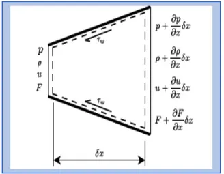
Under the past presumptions and considering the control volume in Figure X, the protection conditions of mass, force and energy can be composed.

Figure 1.2.1: Section of the Duct

The factors present in Figure X speak to: - x, hub facilitate of the pipe; - p, weight;

- ρ, thickness; - u, liquid speed;

- F, cross-sectional region of the channel; - τw, shear weight on the mass of the conduit.

(18)

1.2.1 Equation of Conservation of Mass

The distinction between the mass stream rate leaving the control volume and the mass stream rate entering is equivalent to the rate of progress in mass inside the volume itself.

Revamping condition above and disregarding second request infinitesimals, it is gotten:

1.2.2 Equation of Conservation of Momentum

The whole of the weight powers and the shear powers following up on the outside of the control volume is equivalent to the entirety of the rate of progress of energy inside the control volume and the net efflux of force out of it.

Forces of the Pressure:

Shear stress (f is the friction factor):

The force applied on the lateral wall surface caused by friction: 𝐹 = − 𝑓 ∙1𝜌𝑢2 9𝜌 +𝜕𝜌 𝜕𝑥𝑑𝑥< 9𝑢 + 𝜕𝑢 𝜕𝑥𝑑𝑥< 9𝐹 + 𝑑𝐹 𝑑𝑥𝑑𝑥< − 𝜌𝑢𝐹 = − 𝜕 𝜕𝑡(𝜌𝐹𝑑𝑥) 𝜕𝜌 𝜕𝑡 + 𝜌 𝜕𝑢 𝜕𝑥+ 𝑢 𝜕𝜌 𝜕𝑥+ 𝜌𝑢 𝐹 𝑑𝐹 𝑑𝑥 = 0 𝑝𝐹 − 9𝑝 +𝜕𝑝 𝜕𝑥𝑑𝑥< 9𝐹 + 𝜕𝐹 𝜕𝑥𝑑𝑥< + 𝑝 𝑑𝐹 𝑑𝑥𝑑𝑥 = − 𝜕(𝑝𝐹) 𝜕𝑥 𝑑𝑥 + 𝑝 𝑑𝐹 𝑑𝑥𝑑𝑥 𝜏_A = 𝑓 ∙1 2𝜌𝑢2

(19)

The rate of change of momentum in the volume:

The net efflux of momentum from the control surface:

Taking into account the mass conservation equation, the momentum equation results to be as follows.

G accounts for the viscosity.

1.2.3 Equation of Conservation of Energy

Applying the First Law Thermodynamic to the control volume the protection condition of vitality is inferred.

The protection condition expresses that the contrast between the warmth exchange rate among liquid and pipe through the pipe dividers and the mechanical work rate done by or on the liquid equivalents the entirety of the variety in time of the all out stagnation inside vitality and the net transition of stagnation enthalpy over the control surface. 𝜕(𝜌𝑢𝐹𝑑𝑥) 𝜕𝑡 9𝜌 +𝜕𝜌 𝜕𝑥𝑑𝑥< 9𝑢 + 𝜕𝑢 𝜕𝑥𝑑𝑥< 2 9𝐹 +𝜕𝐹 𝜕𝑥𝑑𝑥< − 𝜌𝑢2𝐹 ≈ 𝜕(𝜌𝑢2_𝐹) 𝜕𝑥 𝑑𝑥 𝜕𝑢 𝜕𝑡 + 𝑢 𝜕𝑢 𝜕𝑥+ 1 𝜌 𝜕𝑝 𝜕𝑥+ 𝐺 = 0 𝐺 = 𝑓𝑢2 2 𝑢 |𝑢| 4 𝐷 𝑄̇ − 𝐿̇ =𝜕𝐸J 𝜕𝑡 + 𝜕𝐻_J 𝜕𝑥 𝑑𝑥

(20)

So as to acquire the last articulation of the vitality protection condition it is important to all the more likely indicate the single terms.

Q ̇ is the warmth entering the control volume through the dividers of the pipe.

q is the warmth traded through the control volume per unit of mass and time;

∆H reaction is the warmth discharged per unit of time and volume by some concoction

responses happening in the gas stream.

(∂E0)/∂t is the variety in time of the all-out stagnation inner vitality.

Where e0 is the particular stagnation vitality:

(∂H0)/∂x is the net transition of stagnation enthalpy through the control surface.

Where the specific stagnation enthalpy is:

At last, presenting an as the speed of sound, considering mass and force conditions, the outflow of the vitality preservation condition results:

𝑄̇ = 𝑞 ∙ 𝜌𝐹𝑑𝑥 + ∆𝐻#NO%&$'(𝐹𝑑𝑥 𝜕𝐸J 𝜕𝑡 = 𝜕(𝑒J𝜌𝐹𝑑𝑥) 𝜕𝑡 𝑒_J = 𝑒 +𝑢2 2 𝜕𝐻_J 𝜕𝑥 = 𝜕(ℎ_J𝜌𝐹𝑢) 𝜕𝑥 𝑑𝑥 ℎ_J = 𝑒_J+𝑝 𝜌 = 𝑐S𝑇 + 𝑝 𝜌 +𝑢2 2 𝜕𝑝 𝜕𝑡 + 𝑢 𝜕𝑝 𝜕𝑥− 𝑎29 𝜕𝑝 𝜕𝑡 + 𝑢 𝜕𝑝 𝜕𝑥< − (𝑘 − 1)𝜌(𝑞 + 𝑢𝐺) = 0

(21)

As per the theory of immaculate gas demonstrate, the speed of sound is given by:

Where T is the temperature, R is the widespread gas consistent and k=cp/cv.

1.3 Conservative Form of Conservation Equations

The framework made by protection conditions speaks to the hyperbolic issue written in non-preservationist shape.

So as to rearrange the goals of the framework, this can be written in moderate shape and after that communicated in lattice frame.

In the traditionalist frame the established energy condition is substituted by the motivation condition which is a direct mix of the mass and the force conditions. It is conceivable to aggregate a few terms and make three vectors.

• Vector of conserved variables

These three factors are autonomous, they shift with x and t and their motions are preserved along the shockwave.

• Vector of conserved variable fluxes

𝑎 = √𝑘𝑅𝑇 ⎩ ⎪ ⎪ ⎨ ⎪ ⎪ ⎧ 𝜕𝜌𝐹 𝜕𝑡 + 𝜕(𝜌𝑢𝐹) 𝜕𝑥 = 0 𝜕(𝜌𝑢𝐹) 𝜕𝑡 + 𝜕](𝜌𝑢2_{+ 𝑝)𝐹^} 𝜕𝑥 − 𝑝𝑑𝐹 𝑑𝑥 + 𝜌𝐺𝐹 = 0 𝜕(𝜌𝑒_J𝐹) 𝜕𝑡 + 𝜕(𝜌𝑢ℎ_J𝐹) 𝜕𝑥 − 𝑝𝑞𝐹 = 0 𝑊` (𝑥, 𝑡) = b 𝜌𝐹 𝜌𝑢𝐹 𝜌𝑒_J𝐹c 𝐹d(𝑊` ) = e 𝜌𝑢𝐹 (𝜌𝑢2_{+ 𝑝)𝐹} 𝜌𝑢ℎ_J𝐹 f

(22)

Mass, drive and stagnation enthalpy transitions are saved through the limits. • Vector of source terms

It is given by the contributes of two vectors. The primary vector contains the source terms because of the variety of the cross segment along the pipe; the second contains the source terms because of the grinding between the liquid and the dividers and to the warmth trade with the liquid.

At long last, the preservation conditions can be written in the conservative frame:

Presently, the framework has three conditions in four obscure (p, u, e, ρ), so a fourth equation is required so as to accomplish solution.

This additional equation must be found in the liquid attributes.

It tends to be embraced the perfect gas model with steady explicit warmth or the mixture of perfect gas model.

On account of gases in motor manifolds and barrels the perfect gas display is, normally, received and the framework is shut by the state condition of perfect gas:

As a matter of fact, this condition presents the gas temperature T as another variable, however for a perfect gas inside vitality and enthalpy are the two elements of the temperature. Along these lines, in the framework the conditions announced underneath must be included.

𝐶̅(𝑊` ) = i 0 −𝑝𝑑𝐹 𝑑𝑥 0 j + b 0 𝜌𝐺𝐹 −𝜌𝑞𝐹c 𝜕𝑊` (𝑥, 𝑡) 𝜕𝑡 + 𝜕𝐹d(𝑊` ) 𝜕𝑥 + 𝐶̅(𝑊` ) = 0 𝜌 𝑝= 𝑅𝑇 𝑒 = 𝑒(𝑇) ℎ = 𝑒(𝑇) + 𝑅𝑇

(23)

If there should arise an occurrence of perfect gas, explicit heat at constant volume cv

and weight cp can be presented, and the past conditions move toward becoming:

Taking everything into account, including conditions of interior vitality and enthalpy to the framework, a shut arrangement of conditions is acquired, described by six free conditions in six questions (p, u, e, ρ, h, T).

The arrangement of this framework combined with the correct limit conditions, decides the stream conditions in any segment of the channel.

1.4 Numerical Techniques

When all is said in done, it is unimaginable to expect to acquire diagnostic answers for the arrangement of fractional differential conditions presented above, so numerical arrangements are required.

So as to decide the variety of all the physical parameters of the liquid in the pipe for each spatial and time condition, it is important to part the continuum liquid mass in a discrete number of littler components shaping a matrix. At that point, the overseeing conditions must be discretized getting to be arithmetical conditions that a PC can comprehend.

The arrangement of these conditions is an obligation of the numerical technique connected.

For quite a while, the Method of characteristic has been utilized, which has a first-arrange precision in reality. In any case, it gives issues in nearness of discontinuities. In this way, later on, this strategy has been substituted by the Shock-capturing technique.

1.4.1 Shock-Capturing Numerical Technique

The numerical arrangement of the protection conditions written in the preservationist shape is figured by Gasdyn utilizing the Shock-capturing strategy in each inside hub of the channels.

𝑒 = 𝑐_S𝑇 ℎ = 𝑐k𝑇

(24)

Along the channels the liquid is exposed to changes in temperature, weight, synthetic piece and to the nearness of stun waves.

Stun waves cause contact discontinuities which lead to discontinuities in the numerical arrangement as well.

The Shock-capturing technique can take care of this issue and give an exact arrangement.

It depends on the application in every hub of the equivalent limited contrasts plot, so as to speak to the spatial subordinate terms.

It is connected to the preservation condition written in conservative network shape X and has a second-arrange precision in the space-time area.

Two changes must be presented:

- the vector W(x, t) is supplanted by Win, which means W(i∆x, n∆t), where the lists I and n are alluded to existence

- the source vectors are erased

along these lines, the Equation X moves toward becoming:

Incorporating X in a network partitioned in ∆x and ∆t networks, Y is obtained.

Along these lines, the previously mentioned issue connected to the logic state of Euler Equations is maintained a strategic distance from, on the grounds that the

𝜕𝑊` 𝜕𝑡 + 𝜕𝐹d(𝑊` ) 𝜕𝑥 = 0 l l 𝜕𝑊` 𝜕𝑡 + 𝜕𝐹d(𝑊` ) 𝜕𝑥 𝑑𝑥𝑑𝑡 = 0 mn∆m m &n∆& & (𝑊`_$(no_{− 𝑊}_` $()∆𝑥 + p𝐹d $no2 ( _{− 𝐹d} $qo2 ( _{r ∆𝑡 = 0}

(25)

indispensable shape can identify the contact discontinuities without knowing their area.

Adjusting the articulation above we can get another plan which speaks to the discretization of nonstop that must be actualized in the technique at limited contrasts.

Summing the distinctions along x:

This articulation above implies that the complete mass, force and vitality at time n+1 breaks even with the whole of the all out mass, force and vitality at time n in addition to the motions through the finishes of the channel. It speaks to a traditionalist discretization conspire.

Specifically, Gasdyn embraces Lax-Wendroff and MacCormack Shock-capturing methods, yet their point by point portrayal is behind the point of this theory.

(𝑊`_$(no_{− 𝑊}_` $() ∆𝑡 + 𝐹d $no₂ ( _{− 𝐹d} $qo₂ ( ∆𝑥 ∆𝑥 s 𝑊`_$(no $,tOm $,t$( = ∆𝑥 s 𝑊`_$( $,tOm $,t$( + ∆𝑡 p𝐹d $no2 ( _{− 𝐹d} $qo2 ( _r

(26)

Chapter 2 Engine Model

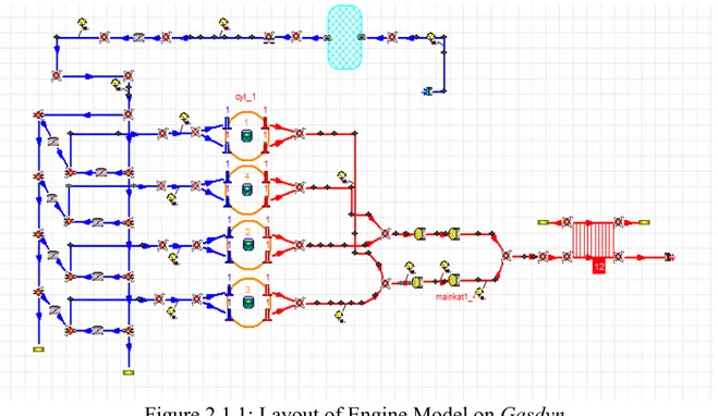
2.1 Layout of the Engine in Gasdyn

The analyzed engine model in this thesis is a SI, four-cylinders, internal combustion engine created by Alfa Romeo.

The engine is normally suctioned and alimented by fuel(gasoline). The Figure 2.1.1 represents the engine schematically in Gasdyn

Figure 2.1.1: Layout of Engine Model on Gasdyn

The air enters from the gulf at the encompassing conditions revealed beneath.

- Temperature: 293 K (20°C)

- Pressure: 1 bar

At that point, it goes through the air channel and the bay conduits (in blue shading) and, in the wake of being metered by the throttle valve, it achieves the four chambers.

(27)

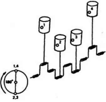
The engine is four-stroke type and the ignition order of the cylinders is 1-4-2-3. Their ignition is moved by 180° crank angle degrees. This is the best demeanor to acquire a customary torque.

Figure 2.1.2: Order of Ignition

The chambers ventilation systems are coupled two by two (1-4 and 2-3) and unite in the pre-impetus, which is trailed by the fundamental impetus.

The impetus is a three-way impetus type.

At long last, the fumes gases experience the silencer and, at that point, they are discharged in the surrounding. The fumes way is set apart in red shading.

The geometry of the considerable number of segments of the motor is now streamlined, so the point of this investigation is executing practical working conditions so as to get in yield right information and, from them, acquiring the plots of the motor maps.

2.2 Combustion Model

The burning model received is a multi-zone Wiebe display.

The principal detail is alluded to the quantity of thermodynamic zone considered for the assessment of thermodynamic properties and compound piece amid the burning. 4 zones have been chosen for this motor.

(28)

The second particular records for the calculation of the consuming rate. 2.2.1 Wiebe Work

The Wiebe work processes the consumed mass division as a component of the wrench edge.

The consumed mass part is given by the proportion between the consumed blend and the complete blend (new in addition to consumed).

xb ranges from 0, toward the start of the burning, to 1, toward the finish of the

procedure, following the law revealed underneath. .

θ is the wrench point variable, θb is the edge that compares to the genuine start of the

burning which is somewhat deferred regarding the start, θe is edge relating to the real end of the ignition procedure.

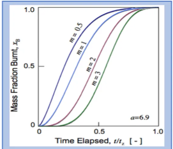
an is the productivity factor, it is a file of the culmination of the burning. In the present motor model an is set to 6,9 which demonstrates a consumed mass part xb = 0.999.

m is the shape factor and it is identified with the speed of the procedure in its underlying stage and it is set to the estimation of 2. m is little if the underlying vitality discharge is high. Both an and m rely upon the geometry of the burning chamber.

𝑥_u = 𝑚u 𝑚_u+ 𝑚_"

𝑥_u = 1 − 𝑒qO9wwqwyqwxx< z{|

(29)

The ordinary pattern of xb against time is S-molded.

Figure 2.2.1: Burnt Mass Fraction Trend

Gasdyn requires the manual presentation of these and different parameters, as per the motor speed.

The decisions embraced are accounted for in the Table 2.2.1.

Table 2.2.1: Burnt Mass Fraction Characteristics

(30)

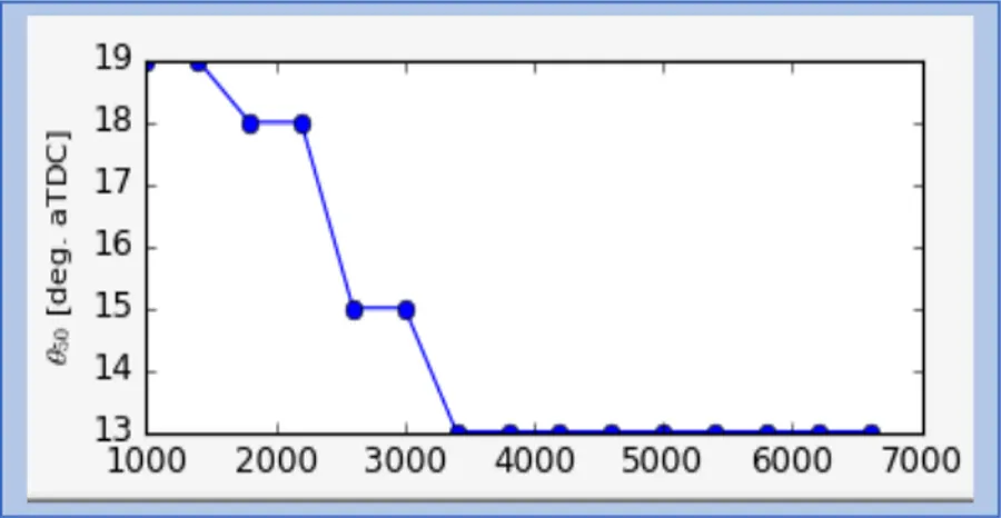
It is additionally called focus of gravity of the burning and it changes as per the speed of the ignition procedure which is quicker at higher motor speed and slower at low rpm. Therefore, higher estimations of θ50 have been set to the most reduced paces. A reference parameter to assess θ50 is the barrel most extreme weight.

This one falls around 20° ATDC (After Top Dead Center) at low rpms and somewhere in the range of 13° and 15° ATDC at higher rpms, as indicated by the patterns of the weight appeared in Figure 2.2.3.

Figure 2.2.2: θ50 vs. Engine Speed

(31)

∆θ10-90 speaks to the length, as far as wrench shaft pivot, of consuming from 10% to

90% of the new charge. It has been settled at 40 degrees.

Inside this interim, the biggest piece of the ignition happens in light of the fact that the fire front is as of now violent and the burning continues quicker.

Then again, the underlying and last parts of the ignition are slower, described by a lower normal consuming rate.

Actually, after the start it requires investment to the fire front to end up totally fierce; while near the finish of the ignition the most piece of the barrel content is made of depleted gases.

Thus, the pattern of xb is S-formed.

2.3 Cylinder Geometry

The geometry of the barrels is a trademark that unequivocally impacts the burning procedure.

Confined rooftop shape with focused start plug has been decided for the burning chamber structure, which is a common decision for barrels with four valves. The focal position of the fitting decides the base conceivable separation for the fire front to spread in every one of the bearings. This prompts a uniform and quick start of the air-fuel blend inside the ignition chamber volume.

In addition, the confined rooftop geometry encourages an effective cross-stream development over the valve cover.

This arrangement demonstrates the most advantageous surface/volume proportion among all the conceivable geometries, because of the way that the head surface accessible is higher.

(32)

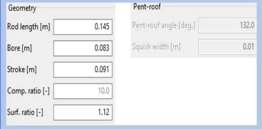
The main dimensions of the cylinders are reported in the figure below.

Figure 2.3.2: Geometry of the Cylinder 2.4 Valves

There are three gatherings of valves present in the model: the throttle valve, 4 valves executed to make the states of the admission variable geometry and the 16 chamber valves.

2.4.1 Throttle Valve

The air suctioned at the admission is compelled to go through the throttle valve arranged after the air channel.

The opening of the throttle valve decides the amount of air that achieves the barrels and blends with fuel, along these lines, in outcome, the heap and the power yield of the vehicle at various working conditions.

It ranges from 0° degrees to 86° degrees, yet the base opening the valve is set to 5°. From 0° to 5° the valve is viewed as shut, while from 86° to 90° totally opened. 2.4.2 Intake Variable Geometry

Along the admission complex of every chamber two valves are available. The opening and conclusion of these valves decides a long or short way for the air entering the chambers.

This technique is utilized to exploit the inertial and wave impacts and improve the chamber filling, with increases in the torque yield.

(33)

Truth be told, without this astuteness, the admission geometry can be advanced just in a constrained speed extend, while a variable geometry is enhanced in a bigger working zone.

The short way is favored for low and high motor rates, while the long way is embraced for medium rpms.

(34)

2.4.3 Valves of a Cylinder

Every chamber of the motor is given four valves, two for the admission a two for the fumes. The Figure 2.4.2 reports the valve timing.

Figure 2.4.2: Valve Timing

The EVO is foreseen before the BDC so as to support the blowdown of the exhaust gases at high pressure and to decrease the work required to the cylinder piston to remove the gas amid the exhaust stroke.

The IVC is deferred after the BDC to permit all the newer charge in the cylinder volume. At the BDC the cylinder piston has completed its intake stroke and it is not any readier to suck extra crisp blend, so the pressure level of the channel pipe, which is higher than the in-chamber pressure at that time, is abused to expand the cylinder filling.

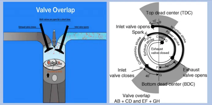
The postponed exhaust valve shutting makes that an overlap period happens, amid which both intake and exhaust valves are kept opened at the same time upgrading the scavenging procedure and the cylinder filling.

(35)

Figure 2.4.3: Valve Overlap

The idleness of the depleted gas leaving the cylinder at high speed helps drawing the new surge into the cylinder chamber.

The overlap time frame is featured in yellow in the plan and must be very much adjusted.

In the event that the overlap is too long the leaving gases could bring a piece of the crisp charge out of the cylinder chamber with them. In the event that, then again, the exhaust gases enter the intake manifold complex they weaken the crisp charge and help decreasing NOx emissions.

2.5 Proportion of Air-Fuel (A/F)

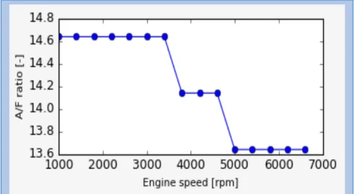
The air-fuel proportion is variable along the speed range of vehicle. This reality unequivocally influences the ignition procedure, and, along these lines, the fuel utilization or consumption and outflows as it will be seen later.

For the engine model considered the stoichiometric estimation of AFR is equivalent to 14.64, the run of the mill an incentive for a SI gas fueled engine.

This AFR esteem has been embraced at low-halfway rpms, which means the rpm interim including ordinary driving conditions.

(36)

More often than not, a stoichiometric AFR is the best decision in wording power creation and of synergist productivity.

In the center scope of the paces a marginally rich blend is utilized, with AFR=14.14. At high rpms the choice of a more extravagant blend has been picked, with an AFR=13.64.

A marginally rich blend is a typical decision for a sparkle start motor in light of the fact that, in this condition, the influence yield is amplified.

(37)

The trend of the variation of the AFR with respect to the engine speed is reported below.

Figure 2.5.2: AFR vs. Engine Speed

2.6 Pollutant Emissions

The primary species engaged with the ignition procedure, for example, H2O, H, H2,

O2, O, OH, CO, CO2, N2 and NO, are processed by Gasdyn in their balance focuses

at consumed gas temperature.

A special case is made for NO and CO, for which kinetic models are considered. The fundamental toxin emanations discharged by a SI motor are CO, HC and NOx, because of the utilization of a stoichiometric or marginally rich air-fuel proportion. The general pattern of the pollutant emissions regarding the AFR is accounted for in Figure 2.6.1.

(38)

Figure 2.6.1: Fuel Consumption and Pollutant Emissions vs. AFR

One of the targets of this proposition is the investigation of the discharges. For this reason, CO, HC and NOx outflow models will be clarified more in detail.

Besides, accordingly of the present consideration on a dangerous atmospheric devation and ecological issues, likewise the CO2 emanations will be researched in this work.

2.6.1 Nitrogen Oxides

NOx arrangement is controlled by the measure of oxygen present in the ignition procedure and by the neighborhood conditions.

It is supported by the utilization of lean blends, described by an abundance of air, and the nearness of high temperature levels.

(39)

The Extended Zel'dovich demonstrate is received to process NOx discharges. It considers just six synthetic responses among all the numerous responses that really happen. O + N₂ ↔ NO + N N + O₂ ↔ NO + O N + OH ↔ NO + H N₂O + O ↔ 2NO N₂O + O ↔ N₂+ O₂ N₂O + H ↔ N₂+ OH 2.6.2 Carbon Monoxides

Carbon monoxide is delivered in correspondence of the fire front as a moderate result of the burning procedure and, contingent upon temperature conditions, can be oxidized and progress toward becoming CO2.

The responses that oversee CO arrangement are accounted for. 𝐶𝑂 + 𝑂𝐻 ↔ 𝐶𝑂₂+ 𝐻

𝐶𝑂₂+ 𝑂 ↔ 𝐶𝑂 + 𝑂₂

In nearness of absence of oxygen, the carbon iotas of the air-fuel mixture are just incompletely oxidized and transform into CO particles. This predominantly happens when rich mixtures are utilized.

The CO equilibrium condition falls amid the fumes gas extension and the cooling stage that pursue the ignition procedure. Here, the nearby conditions decide the incomplete oxidation of CO.

In this work, the Baruah semi-observational model has been embraced to monitor on CO creation.

(40)

This model expect that the most astounding concentration of CO happens at the TDC, where greatest temperature and weight are come to.

Here, CO balance focus is survived and the fixation on CO in the depletes is inferred as pursues.

𝐶𝑂 = 𝐶𝑂_N‚ + 𝑓_ƒ„(𝐶𝑂_tOm − 𝐶𝑂_N‚)

fCO is a remedial factor that ranges from 0, that relates to the balance condition COeq,

to 1, that speak to the most extreme CO arrangement condition COmax. It has been

accepted equivalent to 0.35. 2.6.3 Hydro Carbons

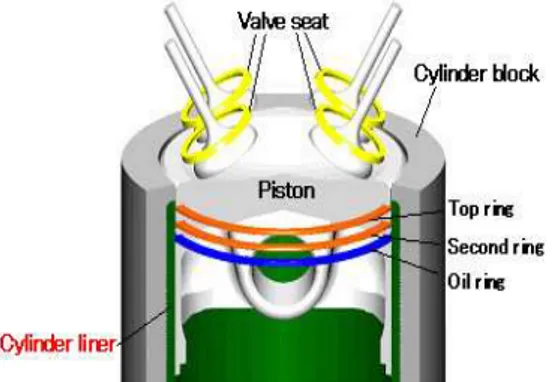
The term HC shows the unburned hydrocarbons, present since part of the air-fuel mixtures gets caught in the crevices or in the grease film.

Hole are limited spaces between chamber liner and cylinder where the fire can't spread because of the warmth exchange to the dividers.

(41)

Amid the compression stroke a specific measure of fresh mixture is constrained in the cleft where it is cooled down because of the heat exchange with the chamber wall. At that point, the combustion decides a quick pressure increment and some more mixture in pushed into the crevice. At the point when the fire front achieves this little volume it extinguishes, at that point the extension stage begins abandoning some unburned particles.

These components are, at that point, discharged and exposed to a moderate post-oxidation process, whose rate is given by an Arrenhius type condition.

Another parameter that impacts this procedure is the position of the sparkle plug, being the fire front considered as spherical.

The other vital reason for unburned HC nearness is the ingestion/desorption of the hydrocarbons in the lubricant.

This system is represented by Henry's Law. The fuel vapor pressure ascends amid the compression stage making great conditions for HC retention in the lubricant oil. The ignition, at that point, drives the vapor concentration to zero and the fuel recently retained is desorbed into the consumed gases.

While in CI engines HC measure of emanations is very little because of the utilization of a lean AFR, in SI they can't be disregarded.

So as to figure HC fixation in the exhaust stream, a few particulars on the geometry of the crevice and the lubricant properties must be set in Gasdyn.

The viability of the post-oxidation process chiefly relies upon gas and cylinder temperatures.

(42)

CHAPTER 3 OptimICE

OptimICE represents Optimizer for Internal Combustion Engine and it is a complex MATLAB®_{code ready to interface with the recreation programming software Gasdyn.} The fundamental capacity is named "optimizer.m", it reviews some different capacities executed in OptimICE and the program Gasdyn and, toward the finish of the running procedure, gives in yield the aftereffects of numerous Gasdyn single recreations.

The utilization of OptimICE reduces profoundly the recreation time since it offers the likelihood to think about all the while the pattern of more parameters in various working states of the engine propelling a solitary simulation.

Initially, the point of the code is the pursuit of the ideal estimations of the primary engine attributes so as to accomplish the most ideal engine arrangement as far as geometry and performances. Along these lines, Gasdyn performances are improved regarding computational time and exactness of the outcomes.

As a matter of fact, the engine model executed in Gasdyn for this thesis is now planned and geometrically streamlined as it has been depicted in the past piece of the work.

In this examination, OptimICE has been utilized with the reason for acquiring a total arrangement of information in regards to the engine performances in the entire agent scope of the vehicle.

3.1 How OptimICE Functions

When the engine model has been stacked on Gasdyn, the information records called input files containing all the data on the engine can be gathered and saved on the pc. The variety of whatever engine parameter produces diverse document inputs.

These documents are perused and explained by OptimICE that, toward the finish of the simulation, gives in yield all the required outcomes situated in numerous folders. For each chosen working purpose (operating point) of the engine an alternate organizer is made.

Furthermore, some other.csv documents are discharged, which outline the estimations of the factors chose at first by the client for each rpm and throttle edge required.

(43)

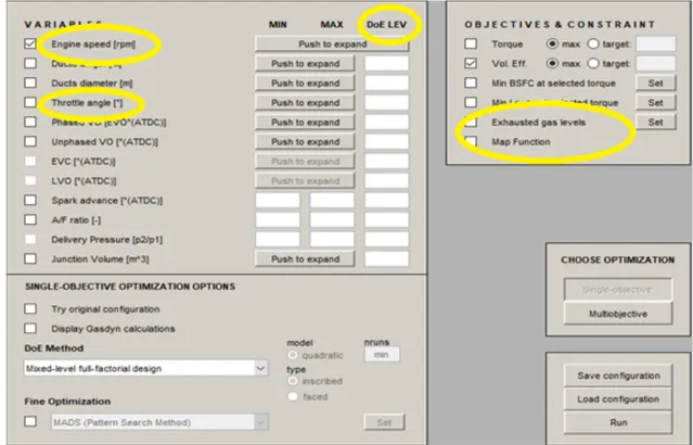
3.2 OptimICE Set-up

The set-up introductory window of OptimICE enables the client to determine the rpms and throttle point openings to recreate or simulate.

For the opening interim of the throttle valve the DoE (Design of Experiments) levels must be determined, it shows in what number of a parts of the opening interim must be separated, by implication characterizing the accuracy of the last outcomes.

Figure 3.2.1: OptimICE Starting Set-Up

In this investigation an interim of 1° angle has been utilized, which is a decent tradeoff between results exactness and computational time.

Furthermore, the client is required to choose the destination of the reenactment. The objective of this thesis is getting information with respect to the fuel utilization and toxin discharge or pollutant emissions. Along these lines, "Exhausted gas levels" and "Map Function" alternatives must be chosen.

In the yield record "FinalResults.csv" all the tried designs are accounted for, with the sort of test executed and the estimations of the fundamental parameters, which means torque, fuel utilization, emanations and volumetric proficiency.

(44)

3.2.1 Motor Speed and Throttle Angle

The variables considered for this project are the motor speed and the opening of the throttle valve.

The engine speed range considered, as indicated by the sort of vehicle contemplated, shifts between 1000 rpm and 6600 rpm, partitioned in interims of 400 rpm.

As of now said previously, the throttle valve is viewed as shut from 0° to 5° degrees. As a first endeavor, a recreation somewhere in the range of 6° and 86° degrees with 81 DoE at 1000 rpm has been led with the point of finding the inert condition. The idle condition is resolved where the engine torque is null, before this esteem the torque is negative and after begins to be positive and having the capacity to offer movement to the vehicle.

For this situation, the main somewhat positive estimation of torque has been found at 9° degrees, so the inert condition is situated somewhere in the range of 8° and 9° degrees.

Thus, the throttle opening considered in the reenactments ranges from 8° to 86° degrees.

By and large, the quantity of working focuses examined is given by the connection: Throttle angles x Engine speeds

So:

79*15=1185

DoE tests are static strategies used to limit the quantity of tests required by the optimization procedure. Amid these tests the factors are, somehow changed and the appropriate response of the framework is considered.

For this situation, the "Mixed level full factorial design" has been utilized, which parts the throttle interim picked in DoE equal interims.

(45)

CHAPTER 4 Maps of the Engine

A engine map is a 2-D plot which reports the pattern of a third factor through isocurves as a component of engine speed and engine torque (or BMEP).

The most widely recognized sort of motor guide demonstrates the iso-utilization curves. Specifically, BSFC (Brake Specific Fuel Consumption) isocurves are plotted that consider just the measure of fuel utilized to create the brake power.

So as to go from engine torque to BMEP the equation reported beneath is utilized, where ε=2, showing a four-stroke motor, and V is the chamber displacement volume.

𝐵𝑀𝐸𝑃 = 𝑃u 𝜔 2𝜋𝜀 𝑉 = 𝑇u 2𝜋𝜀 𝑉

Uniquely in contrast to the torque, the BMEP is free from the cylinder volume, permitting a correlation between various engines.

The iso-utilization map is an imperative reference to assess the execution of a vehicle. Truth be told, the fuel utilization is a list of the effectiveness of the engine work. At equivalent conditions, a lower fuel utilization implies better ignition process, bring down thermo-mechanical misfortunes and less emission discharges.

As a rule, all the engine parameters that change at various working conditions can be plotted in an iso-variable engine map.

Being the principle focal point of the thesis the investigation of utilizations and outflow in various conditions, basically engine maps in regards to these two components will be accounted for and remarked later.

Specifically, there will be talked about the conceivable gains and disservices of utilizing distinctive air-fuel proportions and compression ratios, being these two parameters that emphatically impact crafted by the engine framework.

4.1 Plotting Map of the Engine

So as to most likely draw a decent motor guide it is important to take a shot at the information that OptimICE discharges in yield.

(46)

Actually, all the goal factors, for example, torque, volumetric efficiency, BSFC and emissions, are given as functions of the engine speed and the throttle angle.

The throttle angle opening is certainly not a decent reference to assess the utilizations in light of the fact that the movement of the vehicle is controlled by positive brake torque and BSFC.

At exceptionally low throttle opening the torque can result negative, specifically, at high rpms, thus the BSFC, which is an impossible condition.

Consequently, an approach to go from throttle edge to torque has been idea.

A MATLAB®_{content has been written so as to acquire BSFC and emissions values}

as elements of the motor speed and the torque.

A customized positive torque vector is created, at that point an introduction procedure is connected to the first throttle angles and the new torque, obtaining new estimations of throttle angles relating to the imposed estimations of torque. At last, a second insertion is done between the new throttle openings and the first BSFC, giving another BSFC set of information.

A similar thinking is connected to the discharges.

Along these lines, utilizations and discharges are communicated regarding two invariant vectors containing torque and rpm.

The motor speed go considered is the equivalent before referenced, while the torque run shifts from 1 Nm to the most extreme torque esteem, re-scaling the various factors investigated.

4.2 Engine Maps of the Original Engine Setup

The first engine setup is the one recently presented in the second part.

The motor maps for this design are accounted for toward the finish of the section and will speak to the principal examination term for alternate arrangements.

The BSFC demonstrates a base an incentive around 78 g/MJ, arranged in the fundamental speed range of the vehicle in typical working conditions.

The area of the base BSFC is a basic characteristic for an engine, in light of the fact that the objective of an engine designer of traveler vehicles is to ensure the most minimal conceivable fuel utilization in the principle driving routines. This condition

(47)

enhances the efficiency of the vehicle, comprehensively lessening the expenses and, in addition, the contamination emissions.

Then again, BSFC most extreme esteem has been constrained to 160 g/MJ regardless of whether higher qualities were initially present in the informational index. These cases happened just around inert conditions at low torques, however those numbers were not reasonable.

With respect to emanations, at first sight they appear to expect an uncommon pattern. This reality is especially apparent in CO2, and CO outlines, where the isocurves are

generally hindered in two points.

The clarification must be looked for in the variety of the AFR among the engine speeds.

It changes at 3400 rpm and 4600 rpm, precisely where the plots are interfered. Comparing to these speeds the CO altogether increments, while the CO2 diminishes,

(48)

(49)

Figure 4.2.1: BSFC and Pollutant Emissions of the Original Engine Configuration

(50)

4.3 An Impact of AFR on Engine Maps

The AFR is characterized as the proportion between the mass of air and the mass of fuel associated with the ignition procedure. Its appearance is accounted for in Eq. X.

𝐴𝐹𝑅 =_𝑚𝑚O$#

"ŒN•

So as to see how the air-fuel proportion variety changes fuel utilization and outflows, a similar work improved the situation the first setup has been done with more slender and more extravagant blends.

Reproductions from AFR = 13 to AFR = 16 have been finished expanding the proportion of 0.5each time, being delegate for rich and lean conditions. Moreover, rather than completing a reproduction at AFR = 14.5, the total stoichiometric condition at AFR = 14.64 has been researched.

This time, the isocurves will be more linear due to the reality that constant AFRs have been utilized.

The patterns appeared in Figure 2.6.1 are illustrative of the practices of utilizations and outflows when AFR changes, so they can be utilized as reference to check if the consequences of the reenactments are reasonable and right or not. Some more data can be found additionally in the area 2.6.

* Rich Blend, AFR < 14.64

A mixture is characterized rich when the measure of fuel utilized is higher than the stoichiometric.

Not surprisingly, the BSFC is higher than the first case, in light of the fact that a greater measure of fuel is sustained in every chamber.

The littler amount of air, and therefore oxygen, accessible decides the varieties of the discharges.

CO creation essentially increments on the grounds that a lower measure of fuel is totally oxidized. This perception legitimizes likewise the CO2 decrease.

Unburned HC ascend as the blend gets more extravagant in light of the fact that there isn't sufficient air to consume all the fuel.

(51)

* Lean Blend, AFR > 14.64

A blend is lean when an overabundance of air is available.

Contemplations like those communicated for the rich blend case can be connected to this case, clearly acquiring inverse outcomes.

More consideration must be paid for the lean condition, in light of the fact that, while every one of the factors in the rich case expect a monotonic conduct as the AFR diminishes, expanding the AFR the bends, after specific qualities, change their behaviour.An exemption happens for the CO that turns out to be practically

unimportant in nearness of extremely lean blends. Truth be told, the CO plot on account of AFR=16shows CO focuses near zero.

* Stoichiometric Blend, AFR = 14.64

A blend is characterized as stoichiometric when the correct measure of air important to consume a unit of fuel is encouraged to the barrels.

The left piece of the plots (low rpm) is equivalent to the first design, at that point they expect the conduct of the lean blend case.

In the accompanying pages the motor maps of BSFC, CO, CO2, NOx and HC are connected after expanding estimations of AFR. For each condition 10 plots are accounted for in two unique pages, the initial 5 are the previously mentioned variable patterns, the seconds report the percent variety between the first AFR and the thought about one.

(52)

(53)

(54)

(55)

(56)

(57)

(58)

(59)

(60)

(61)

(62)

(63)

Figure 4.3.6: BSFC and Pollutant Emissions Difference Percentage Between the Original Configuration and AFR=14.64

(64)

(65)

(66)

(67)

(68)

(69)

(70)

(71)

(72)

(73)

4.4 CR impact on Engine Maps

The geometrical CR is characterized as the proportion between the complete volume of the cylinder, given by the total of ignition chamber and uprooting volume accessible when the cylinder is at the BDC, and the burning chamber volume, which is the base volume accessible among the procedure in correspondence of the cylinder at the TDC.

The successful CR can be not the same as the geometrical one. 𝐶𝑅 =𝑉%%+ 𝑉Ž

𝑉_Ž =

𝑉&'&

(74)

Figure 4.4.1: Cylinder Geometry and CR Features

The first compression ratio of the Alfa Romeo engine is set to 10.

In this segment it will be discussed about the impact of higher CRs on fuel economy and discharges.

For the most part, any expansion of the CR prompts higher thermal effectiveness, because of an increasingly total combustion. This is because of the way that the fuel in the cylinder chamber faces higher temperature and pressure conditions.

A correlation between these two parameters is accounted for in Figure 4.4.2 and Figure 4.4.3.

The brake thermal efficiency is entirely associated with the fuel utilization which diminishes as the BTE rises.

Another essential angle is connected to the CR: as the CR expands the CO2

emanations decline.

Because of the current stringent points of confinement on emanations, specifically on CO2, the CR control is entirely examined. A few points of confinement and

(75)

The raise of CR suggests higher mechanical and warm burdens and vibrations, requiring an increasingly hearty and exorbitant cylinder chamber gear.

Regardless, high temperatures and pressures upgrade the inclination of thump supporting the early auto-ignition of the blend.

Another issue associated with the temperature is the gigantic increment of NOx emissions, because of the high temperatures.

In this work, the consequences of expanding the CR from 10 to 14 have been contemplated.

Beginning from CR = 12 a geometrical modification necessary, that is expanding the squish width shape 10 mm to 15 mm.

Positive outcomes as far as BSFC decrease are accomplished primarily at full-stack conditions and comparing to middle of the road/high throttle opening and torques, while CO2 fixation is bringing down in practically every one of the conditions.

(76)

(77)

(78)

(79)

(80)

(81)

(82)

(83)

(84)

(85)

(86)

(87)

(88)

(89)

(90)

(91)

(92)

(93)

(94)

(95)

(96)

(97)

(98)

(99)

(100)

(101)

(102)

(103)

(104)

(105)

(106)

4.5 Atkinson Cycle

The Atkinson Cycle, admired in the nineteenth century by James Atkinson, speaks to another technique expected to decrease the BSFC. This system is utilized by numerous famous vehicle brands, for example, Toyota and Mazda, particularly in the classes of mixture or turbocharged vehicles.

Anyway, this thought has been adjusted additionally to motor case contemplated in this postulation, regardless of whether it is a SI normally suctioned motor, so as to check whether any beneficial outcome can be abused as well.

The fundamental goal of the Atkinson Cycle is developing the extension stage deferring the admission valve conclusion (LIVC, Late Intake Valve Closure), making the power stroke longer than the pressure stroke and accomplishing an over-development of the liquid caught in the barrel.

Another approach to apply the Atkinson Cycle is the EIVC (Early Intake Valve Closing), however in this work just the LIVC will be explored.

Figure 4.5.1: LIVC and EIVC Configurations

As per the definition, the LIVC is abused shutting the delta valves some wrench degrees after that the cylinder has achieved the BDC. Along these lines, some portion of the crisp blend that has just entered in the barrel returns into the admission complex making that the pressure stroke results shorter.

So as to research on the advantages of the Atkinson Cycle, LIVC system has been actualized in the motor contemplated.

(107)

This gadget has been combined with the expansion of the CR, permitted on the grounds that LIVC lessens the likelihood of thump on account of the most extreme temperature decrease. A CR equivalent to 13 has been embraced for the reproductions.

The outcomes demonstrate the enhancement of the BTE because of the over-extension, regardless of whether just at high motor rates.

This result was unsurprising in light of the fact that at low speeds the chamber filling coefficient is lower and the break of some increasingly crisp charge does not create any focal points.

The quirk of the Atkinson cycle is the capacity of better misusing the vitality naturally hold by the consumed gases at high weight. It recoups the vitality lost at the EVO in a traditional Otto, as Figure X schematically appears.

The picture is a bit veering off in light of the fact that, regardless of whether the characteristic vitality hold by the hot gas is better misused, the power yield is all inclusive lower because of the littler measure of gas consumed.

The BTE is characterized as the proportion between the brake control and the lower warming estimation of the fuel.

𝐵𝑇𝐸 =𝑃u#O•N

𝐿𝐻𝑉 =

𝑃_$(Ž$%O&NŽ − 𝑃_{"#$%&$'( •'••} 𝐿𝐻𝑉

Figure 4.5.2: Comparison Between the Ideal Indicated Cycles of an Otto Cycle and Atkinson Cycle

(108)

4.5.1 LIVC Incitation

To get the LIVC the bay valves lift law is balanced so as to keep the valves opened amid the admission stroke as well as amid part of the pressure stroke for some wrench degrees after the BDC.

The development of the cylinder toward the TDC drives some portion of the new blend back to the admission channel, decreasing the first measure of charge inside the barrel and, as a result, the powerful CR.

The new lift law holds the first IVO and forces a more extended term.

On a basic level, the valve lift is controlled by the structure of the camshaft, which is associated with the crankshaft through a belt or a chain in such an approach to have a pivot speed lower than the motor shaft.

The Figure X indicates schematically how the cam projection geometry influence the valve lift managing, in mix with the motor speed, the contact time between the cam and the valve tappet.

Figure 4.5.3: Cam Geometry Influence on Valve Lift

Current vehicles are typically furnished with complex cam frameworks to accomplish a Variable Valve Timing (VVT) enhanced for every one of the routines.

Gasdyn, does not require a manual mediation on the cam geometry, yet just another admission valve lift law in info.

(109)

enhanced one. For this last an amplification of 20° in the focal piece of the valve lift has been done, comparing to a more extended greatest lift interim.

Figure 4.5.4: Valve Timings of the Original Engine Configuration and the Atkinson Configuration

This modification prompts an enhancement in the BTE at high rpms, as per the past contemplations, as it tends to be found in Figure 4.5.5.

(110)

Figure 4.5.5: BTE Comparison Between the Original Engine Configuration and the Atkinson Configuaration

(111)

A higher BTE is a list of a superior burning procedure, which prompts bring down BSFC and CO2 discharges.

BSFC decreasesmainly at halfway high torques; this proof recommends the implemetation of the LIVC just in certain working ranges.This proof clarifies the previously mentioned execution of VVT frameworks.

BSFC and CO2 charts are accounted for toward the finish of this passage.

The primary disadvantage is spoken to by a lower control thickness, which legitimizes the implementetion of Atkinson cycle in the half breed vehicles that can remunerate the power yield with the electric engine.

This is an undesired impact of the lower compelling dislodging volume which is connected the measure of caught blend. This is appeared in the near plot in Figure 4.5.6, where the first and Atkinson Pressure-Volume cycles are covered.

Figure 4.5.6: Comparison Between the Indicated Cycles of the Original Engine Configuration and the One With the LIVC

(112)

(113)

Figure 4.5.7: BSFC Comparison Between the Original Configuration (first graph) and the One with LIVC (second graph)

(114)

Figure 4.5.8: CO2 Comparison Between the Original Configuration (first graph)