1
CHAPTER ONE
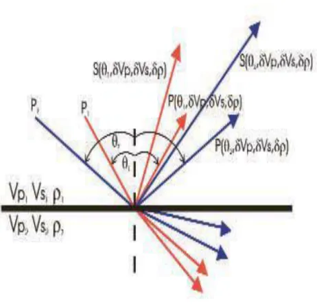
1.1 INTRODUCTION TO AVO ANALYSIS 1.1.1BACKGROUND
Seismic amplitude-versus offset (AVO) analysis has been a powerful geophysical method in aiding the direct detection of gas from seismic records. This method of seismic reflection data is widely used to infer the presence of hydrocarbons. The conventional analysis is based on such a strategy: first, one estimates the effective elastic parameters of a hydrocarbon reservoir using elastic reflection coefficient formulation; which models the reservoir as porous media and infers the porous parameters from those effective elastic parameters. Strictly speaking, this is an approximate approach to the reflection coefficient in porous media. The exact method should be based on the rigorous solutions in porous media. The main thrust of AVO analysis is to obtain subsurface rock properties using conventional surface seismic data. The Pooisson‟s ratio change across an interface has been of particular interest. These rock properties can then assist in determining lithology, fluid saturants, and porosity. It has been shown through solution of the Knott energy equations (or Zoeppritz equations) that the energy reflected from an elastic boundary varies with the angle of incidence of the incident wave (Muskat and Meres, 1940). This behavior was studied further by Koefoed (1955, 1962): He established in 1955 that, the change in reflection coefficient with the incident angle is dependent on the Poisson‟s ratio difference across an elastic boundary. Poisson‟s ratio is defined as the ratio of transverse strain to
longitudinal strain (Sheriff, 1973), and is related to the P-wave and S-wave velocities of an elastic medium by equation 1 below. Koefoed in 1955 also proposed analyzing the shape of the reflection coefficient vs. angle of incidence curve as a method of interpreting lithology.
2 1 1 2 1 2 2 Vs V Vs V p p
... (1)In 1984, Ostrander introduced a practical application of the amplitude variation with incident angle phenomenon. He used the Zoeppritz amplitude equations (e.g. Aki and Richards, 1980) to analyze the reflection coefficients as a function of the angle of incidence for a simple three-layer, gas-sand model. The model consisted of sand layer encased in two shale layers. By using published values of Poisson‟s ratio for shale, brine saturated sands, and gas saturated sands, he determined that there is a significant enough change in reflection coefficient with angle of incidence to discriminate between gas saturated sands and brine saturated sands. He tested his theoretical observations with real seismic data and determined that AVO could be used as a method of detecting gas sands (Coulombe et al., 1993). AVO analysis in general, is limited by the assumptions and approximations inherent in surface seismic acquisition, processing, and interpretation. These factors include receiver arrays, near surface velocity variations, differences in geometrical spreading from near offset to far offset, dispersive phase distortion, multiples interfering with primaries, wavelet phase, source directivity and array effects (pers. Comm. R. R. Stewart, 1990). In addition, AVO analysis requires accurate determination of the angle of incidence at an interface, the accuracy of which depends on an accurate velocity model (Coulombe et al., 1993).
This method (AVO) can be explained by using this example, A 48 fold 3D seismic survey is divided into 48 constant-offset components. Each constant-offset component can be migrated (using the correct velocities) to produce a volume, giving the image of the subsurface. Each of the 48 cubes gives the same image, except that the amplitudes are different. At the same point in
3
all the 48 volumes the variation of the seismic amplitude with offset, h, is referred to as AVO information. The variation in amplitude can be fitted in this form of function (amp = A + Bsin2θ), where A is the intercept of AVO, B is the AVO gradient and θ is the angel of incidence. In practical world, both the estimated intercept and the gradient volumes are used in locating gas fields and other anomalies. (Rutherford et al., 1989).
The conventional treatment of seismic data, however, masks the fluid information. This problem lies with the way seismic traces are manipulated in order to enhance reflection visibility. In a seismic survey, as changes are made in the horizontal distance between source and receiver, called offset, the angle at which a seismic wave reflects at an interface also changes. Seismic traces-recordings of transmitted and reflected sound are sorted into pairs of source-receiver combinations that have different offsets but share a common reflection point midway between each source-receiver pair. This collection of traces is referred to as a common midpoint (CMP) gather. In conventional seismic processing, in which the goal is to create a seismic section for structural or stratigraphic interpretation, traces in a gather are stacked-summed to produce a single average traces. (Chiburis et al., 1993).
1.2 WHAT IS AMPLITUDE VERSUS OFFSET/ANGLE (AVO/AVA)
In geophysics, amplitude versus offset (AVO) or amplitude variation with offset is a variation in seismic reflection amplitude with change in distance between shot point and receiver that indicates differences in lithology and fluid content in rocks above and below the reflector. It is also referred as AVA (amplitude variation with angle). As AVO studies are being done on CMP data, the offset increases with the angle ( Schlumberger Oilfield Glossary).
4
An AVO anomaly is most commonly expressed as increasing (rising) AVO in a sedimentary section, often where the hydrocarbon reservoir is "softer" (lower acoustic impedance) than the surrounding shale. Typically amplitude decreases (falls) with offset due to geometrical spreading, attenuation and other factors. An AVO anomaly can also include examples where amplitude with offset falls at a lower rate than the surrounding reflective events (Schlumberger Oilfield Glossary). In theory, as the AVO phenomena translates the sharing of the energy of the incident compressible wave between the compressible and converted reflections, the observation of the converted mode AVO would be redundant. In some privileged areas, the AVO of compressible waves effectively provides the expected information. In most cases, single fold data are not pure enough to provide reliable amplitude measurements, and finally the result will be doubtful (Xu, Y and Bancroft, J. C., 1997)
1.2.1 SEISMIC ENERGY PORTIONING AT BOUNDARIES
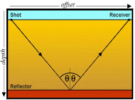
Amplitude variation with offset comes about from something called „energy partitioning‟. When seismic waves hit a boundary, part of the energy is reflected while part is transmitted. If the angle of incidence is not zero, P wave energy is partitioned further into reflected and transmitted P and S components. The amplitudes of the reflected and transmitted energy depend on the contrast in physical properties across the boundary. For seismic people, the important physical properties in question are compressional wave velocity (Vp), shear velocity (Vs) and density (ρ). But, the important thing to note is that reflection amplitudes also depend on the angle-of-incidence of the original ray as shown in the figure 1
5
Fig 1: A seismic wavefront hitting a reflector. The physical properties are different on either side of the reflector.
How amplitudes change with angle-of-incidence for elastic materials is described by the quite complicated „Zoeppritz equation (as well as higher-level approximations like that of Aki and
Richards in their famous seismology textbook of 1979). But there are many different simplications of these equations that make analysis of amplitudes with angle much easier. One thing to point out now is that „amplitude variation with offset‟ is not always an appropriate term. For proper analysis, we need „amplitude variation with angle‟.
The Zoeppritz equations describe the reflections of incident, reflected, and transmitted P waves and S waves on both sides of an interface. For analysis of wave reflection we need an equation
6
which relates reflected wave amplitudes to incident wave amplitudes as a function of angles of incidence. In the past decade, many forms of simplifications of Zoeppritz equation of P-P reflection coefficient appeared in the literature and industrial practice (Aki and Richards, 1980, Shuey, 1985, Parson, 1986, Smith and Gidlow, 1989, Verm and Hilterman, 1994). Each of these simplifications in a degree links reflection amplitude with variations of rock properties. Aki and Richards (1980) give the approximation of P-S reflection coefficient. There is also a rough approximation linking P-S reflection coefficient with pure SH reflection coefficient (Fraiser and Winterstein, 1993, Stewart, 1995). Because of the challenges in the processing of the real radial data which are mainly P-S reflections, applications of P-S reflection coefficient and AVO analysis rarely appear in the literatures and practice (Xu, Y and Bancroft, J. C., 1997).
1.2.2 MECHANICS OF QUANTITATIVE AVO ANALYSIS.
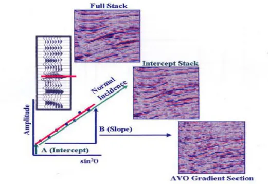
Quantitative AVO analysis is done on midpoint-gathers (or super-gathers, or common-offset gathers, or as they are called in the AVO business „Ostrander gathers‟ (Ostrander 1984). At each time sample amplitude values from every offset in the gather are curve-fit to a simplified, linear AVO relationship as in Figure 2. A better way of saying this is that we fit a best-fit straight line to a plot of amplitude versus some function of the angle of incidence. This yields two AVO attributes-basically the slope and intercept of a straight line, which describes, in simpler terms how the amplitude behaves with angle of incidence. There are a lot of equations that have been used over the last 15 years or so, but all of them, no matter what interpretation is given to the „intercept‟ and „slope‟, work in this same way.
7 1.3 THEORY OF AVO/AVA
Basic AVO theory is well understood because it is widely used as a tool in hydrocarbon detection (Smith, 1987). A few of the most important ideas will be highlighted to keep in mind when doing AVA analysis. Figure 1 above shows the theoretical energy partition at an interface. This figure illustrates an important point that accounts for AVA phenomena: the conversion of P-wave energy to S-P-wave energy. Though the majority of seismic data is recorded simply as a single component pressure wave, the fact that the Earth is elastic causes amplitudes of P-wave arrivals to be a function of S-wave reflection coefficient (Rs) (Castagna, J. P., and Smith, S.W., 1994). In practice, Rs is tricky to obtain and the P-wave reflection coefficient (Rp) is what we have in the vast majority of cases (Smith, G.C., and Sutherland, R.A., 1996).
Several attempts at the practical application of AVO began about 15years ago, but the physics draws on 19th century advances in optics and electromagnetic wave theory. Green and Kelvin made some speculation about the similarity of the reflective behavior of light and elastic waves in the 1800s (Green 1871). Using Snell‟s law, Knott in 1899, and Zoeppritz in 1919, developed general expressions for the reflection of compressional and shear waves at a boundary as a function of the densities and velocities of the layers in contact (Knott 1899 and Zoeppritz 1919). Although Zoeppritz was not the first to publish a solution, his name is associated with the cumbersome set of formulas describing the reflection and refraction of seismic waves at an interface. In 1936, Macelwane and Sohon recast the equations to gain insight into the physics and facilitate calculations (Macelwane et al 1936). Before the advent of computers, AVO effects
8
were incorporated into synthetic seismograms and other calculations using approximated Zoeppritz equations (Muskat et al 1940, Koefod 1955 and Bortfeld 1961). Today, personal computers can generate synthetics based on the full Zoeppritz formalism, but approximations are still used to gain physical insight into the relative influence of velocity and density changes on seismic amplitudes, and in the attempt to back out lithology and fluid type from AVO data (Aki et al 1980).
1.4 APPLICATION OF AVO/AVA
AVO has its most common application in hydrocarbon reservoirs , i.e. it is used by geophysicists to determine thickness, porosity, density, velocity, lithology and fluid content of rocks. For successful AVO analysis, special processing of seismic data and seismic modeling is needed to determine rock properties with a known fluid content. This knowledge makes it possible to model other types of fluid content. A gas-filled sandstone might show increasing amplitude with offset, whereas a coal might show decreasing amplitude with offset. AVO rising is typically seen in oil-bearing sediments, and even more so in gas-bearing sediments. Particularly important examples can be observed in turbidite sands such as the Late Tertiary deltaic sediments in the Gulf of Mexico (especially during the 1980s-1990s), West Africa, and other major deltas around the world. AVO is most routinely used by most major companies as a tool to "de-risk" exploration targets and to better define the extent and the composition of existing hydrocarbon reservoirs.
In AVO analysis, practices mainly focus on looking for more sensitive indicator of hydrocarbon and extracting and exploiting anomalous variations between seismic and these
9
sensitive parameters. Some authors (Goodway et al., 1997) showed the advantages of converting velocity measurements to Lame‟s moduli parameters (λ and μ) to improve identification indicator of reservoir zones. Castagna et al (1985) observed a few relationships of compressible wave and shear wave in the elastic silicate rocks. These give us good empirical guidance to study the rock property from seismic data.
Least square regression analysis an inversion is the common approaches in the AVO analysis. In 1986, Parson obtained contrasts of three elastic parameters (λ, μ and ρ) by pre-stack inversion. Goodway et al (1997) obtained the Vp and Vs from inversion and converted them to the λ/ μ to detect the reservoirs. However, the non uniqueness is always the problem in the seismic inversion. The background velocity error causes the ratio to change greatly or eliminates the high frequency contrast. Appropriate selection of parameters, background velocity, wavelet estimation, application of a priori information is still important issues which remain to be resolved. The least square regression analysis is used to extract elastic parameters from pre-stack data. The extraction provides band-limited information on which attempt to discover anomaly caused by hydrocarbon reservoirs (Xu, Y and Bancroft, J. C., 1997).
An important caveat of AVO analysis using only P-energy is its failure to yield a unique solution, so AVO results are prone to misinterpretation. One common misinterpretation is the failure to distinguish a gas-filled reservoir from a reservoir having only partial gas saturation ("fizz water"). However, AVO analysis using source-generated or mode-converted shear wave energy allows differentiation of degrees of gas saturation. Not all oil and gas fields are
10
associated with an obvious AVO anomaly (e.g. most of the oil found in the Gulf of Mexico in the last decade), and AVO analysis is by no means a panacea for gas and oil exploration.
1.5 PROBLEM STATEMENT
In the late 1920s, the seismic reflection technique became a key tool for the oil industry, revealing shapes of subsurface structures and indicating drilling targets. This has developed into a multibillion dollar business that is still primarily concerned with structural interpretation. But advances in data acquisition, processing and interpretation now make it possible to use seismic traces to reveal more than just reflector shape and position. Changes in the character of seismic pulses returning from a reflector can be interpreted to ascertain the depositional history of a basin, the rock type in a layer, and even the nature of the pore fluid. This last refinement, pore fluid identification, is the ultimate goal of AVO analysis.
Amplitude variation with offset, AVO, has become an essential tool in the petroleum industry for hydrocarbon detection (Rutherford and Williams, 1989). AVO responses vary depending on the physical parameters of the reflection interface and incidence angle (Shuey, 1985). In relatively simple geologic settings, offset is a simple function of angle (Castagna and Smith, 1994). However, a more realistic V (z, m) will make offset and incidence angle a complex relation (Sheriff, 1995). In these settings, amplitude variation with angle (AVA) is a preferable alternative to AVO analysis. Among the various seismic technique for hydrocarbon detection and monitoring in the subsurface, Amplitude variation with offset (AVO) methods appear to be quite promising. The AVO is measured in the primary P-wave
11
reflections, which are the strongest and freest from contamination, and at the same time, they contain the information about the S-wave reflectivity. Many theoretical models were established based on AVO equations in fluid-gas media; however, still little research has been done on time-lapse AVO attributes in real data. It is therefore necessary to perform further research on the use of AVO analysis on seismic data.
1.6 JUSTIFICATION OF THE THESIS.
Early practical evidence that fluids could be seen by seismic waves came from “bright spots”- streaks of unexpectedly high amplitude on seismic sections, often found to signify gas. Bright spots were recognized in the early 1970s as potential hydrocarbon indicators, but .drillers soon learned that hydrocarbons are not the only generators of bright spots. High amplitudes from tight or hard rocks look the same as high amplitudes from hydrocarbons, once seismic traces have been processed conventionally. Only AVO analysis, which requires special handling of the data, can distinguish lithology changes from fluid changes. (Chiburis et al., 1993).
It has been two decades, for the quick development in seismic exploration. AVO technology has remarkably advanced and has been extensively implemented in oil industry. Nevertheless, the Zoeppritz equation considers only the elastic properties of the rocks ignoring the non elastic properties such as velocity dispersion attenuation. Considering all these things, there are still problems that the traditional AVO technology is not able to handle adequately.Over the period of time, Geophysicists have noticed low-frequency seismic anomalies associated with hydrocarbon reservoirs and this topic is gained more and more attention.
12
The great promise of amplitude-versus-offset (AVO) analysis lies in the dependence of the offset-dependent-reflectivity of reflected compressional waves on the elastic properties of the subsurface. As different lithologies may exhibit distinct Poisson‟s ratios and gas bearing strata usually exhibit anomalously low Poisson‟s ratios. AVO has been recognized as a potential
seismic lithology tool and direct hydrocarbon indicator. Unfortunately, experience has shown that the theoretical potential for AVO analysis is, all too often, not realized in practice. Despite some notable successes, it cannot be claimed that economic impact of AVO analysis is on a par with other breakthrough in geophysical technology such as a bright spot analysis or 3D seismic surveys. This lack of penetration of AVO into the mainstream as an interpretation technology is not due to any inherent lack of validity of the concept, but rather due to a lack of credibility of the concept in the minds of potential practitioners (Castagna, 1995).
The purpose of this thesis is to consider the basics of amplitude variations with offset (AVO). It will also be demonstrating the idea that changes in seismic amplitude with offset (AVO effects) are due to contrasts in the physical properties of rocks. Moreover, further, quantitative analysis of AVO effects can yield attributes that discriminate between lithologies and fluids. Further analysis can also lead directly to estimates of the elastic properties that will give rise to the AVO effects and also reduce the uncertainties of interpretation.
1.7 RESEARCH OBJECTIVES
1. The basic goal in this study is to obtain subsurface rock properties using conventional surface seismic data.
13
3. To use AVO analysis to predict the characteristics of a reservoir and to make a preliminary determination of the type of material and its detectability of its AVO response.
4. To look at the physical cause of AVO behavior.
14
CHAPTER 2
LITERATURE REVIEW
2.1 INTRODUCTION
Considering the conventional utilization of the seismic reflection method, it has been assumed traditionally that seismic signals can be viewed as a band-limited normal incidence reflection coefficient series with appropriate travel time and amplitude variation due to propagation through an overload. It has been demonstrated that gas sand reflection coefficient vary in anomalous fashion with increasing offset, it also displayed how to utilize this anomalous behavior as a direct indicator of hydrocarbons in relation to real data (Ostrander, 1982). This work done by Ostrander made the methodology commonly known as amplitude variation with offset analysis (AVO) very popular. Moreover, this method is not only “Seismic lithology” but it also provides an enhanced model of the reflection seismogram which allows one to better estimate both “background velocities” and normal incidence reflection (Castagna, 1993).
Exploration geophysics can be considered as a science of anomalies to a considerable extent. Most of the hydrocarbons discovered about fifty years ago can safely be assumed to be associated with some kind of geophysical anomaly. Explorationists routinely make use of deviations from expected gravity, seismic travel time and seismic amplitude without recovering uniquely determined absolute density, depth or reflectivity. Consequently, significant risk is associated with drilling a well, even when all the technology and analysis available have been thrown at the problem. Experience has shown that geophysical anomalies can be used to reduce risk, and consequently, to identify new prospects (Castagna, 1993).
15
Thus, one would expect the exploration geophysicist, who is concerned primarily with finding hydrocarbons, to have somewhat different expectations from AVO analysis, than say a research physicist, who may be primarily concerned with getting the right answer. Taking the latter approach, if one makes very simplistic assumptions, methods can be developed which work well on synthetic data. However, the more one appreciates the complexities of the real world with real geology, the more it becomes apparent that AVO analysis does not work. The only negative side of this conclusion is that, people are successfully still using AVO anomalies to find hydrocarbons throughout the world. The geophysicist does not require answers that are absolutely correct, acceptable range of deviations from some background trend may be sufficient for instance the magnitude of the deviation in absolute units may not even be required. A very vivid analogy is the spontaneous potential (SP) log. If one is told that an SP log reading is -30 millivolts at some depth, the rock properties cannot be interpreted from this even with the most complex modeling and inversion schemes. This is because the SP log is an anomaly log with no meaningful absolute scale. When it is noted that 30 millivolts is quite a phenomenal deviation from the background trend which is produced by surrounding shale, It can be said that the SP log is very important in identifying sands (Castagna, 1993).
2.2 PRINCIPLES OF AVO/AVA.
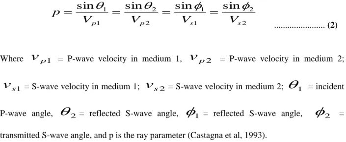
In exploration geophysics, simple isolated interfaces are scarcely dealt with. However, our understanding of offset-dependent reflectivity must begin with portioning of energy at just such interface (Castagna and Backus, 1993). In the Figure below, the angles of incident, reflected and transmitted rays synchronous at the boundary are related according to snell‟s law by:
16 2 2 1 1 2 2 1
1
sin
sin
sin
sin
s s p pV
V
V
V
p
... (2)Where
v
p1 = P-wave velocity in medium 1,v
p2 = P-wave velocity in medium 2;1 s
v
= S-wave velocity in medium 1;v
s2 = S-wave velocity in medium 2;
1 = incident P-wave angle,
2 = reflected S-wave angle,
1 = reflected S-wave angle,
2 = transmitted S-wave angle, and p is the ray parameter (Castagna et al, 1993).Fig 2. Reflection and transmission at an interface between two infinite elastic half-spaces for an incident P-wave (Castagna et al, 1993).
17
The P-wave reflection coefficient as a function of incidence angle Rp p1 is defined as the ratio of the amplitude of the reflected wave to that of the incident wave. Similarly, the
P-wave transmission coefficient Tp p
1
is the is the ratio of the amplitude of the transmitted P-wave to that of the incident P-wave. Also, Rp s
1 is the ratio of theamplitudes of reflected S-wave and incident P-waves, and Tp s
1 is the ratio of thetransmitted S-waves amplitudes of transmitted S-waves and incident P-wave amplitudes. The following discussion is for particle displacement amplitudes, with polarity assigned according to the horizontal component of displacement.
At normal incidence, there are no converted S-waves and the P-wave reflection coefficient Rp is given by
2 1
1 2 1 2 / 2 1 2 1 p p p A p p p p p p In I I I I I I I I R ... (3)Where Ip is the continuous P-wave impedance profile.
Ip2 = impedance of medium 2 = ρ 2V ρ 2 ρ 2= density of medium 2. Ip1= Impedance of medium 1 = ρ 2V ρ 2 ρ 1= density of medium 1.
18
Ip Ip2 Ip1 ... (4) The logarithmic approximation is acceptable for reflection coefficients smaller than about + 0.5.
The P-wave transmission coefficient at normal incidence Tp is given by
Tp = 1 - Rp. ... (5)
The variation of reflection and transmission coefficients with incident angle (and corresponding increasing offset) is referred to as offset-dependent-reflectivity and is the fundamental basis for amplitude-versus-offset analysis (Castagna et al, 1993).
Knott (1899) and Zoeppritz (1919) invoked continuity of displacement and stress at the reflecting interface as boundary conditions to solve for the reflection and transmission coefficients as functions of incident angle and the elastic properties of the media (densities, bulk and shear moduli), though the resulting Knott and Zoeppritz equations are notoriously complex. Aki and Richards (1980) and Waters (1981) gave an easily solved matrix form
Q
P
R
1
... (6)
Where Q, P, and R in Appendix A (Castagna and Backus, 1993).
In 1995, Koefoed first showed the practical possibilities of using AVO analysis as an indicator of Vp/Vs variations and empirically established five rules, which were later verified by shuey in 1985 for moderate angles of incidence (Zhang et al, 2001):
a) When the underlying medium has the greater longitudinal [P-wave] velocity and other relevant properties of the two strata are equal to each other, and increase of Poisson‟s
19
ratio for the underlying medium causes an increase of the reflection coefficient at the larger angles of incidence.
b) When, in the above case, Poisson‟s ratio for the incident medium is increased, the reflection coefficient at the larger angles of incidence is thereby decreased.
c) When, in the above case, Poisson‟s ratio for both media are increased and kept equal to each other, the reflection coefficient at the larger angles of incidence is thereby increased.
d) The effect mentioned in (1) becomes more pronounced as the velocity contrast becomes smaller.
e) Interchange of the incident and the underlying medium affects the shape of curves only slightly, at least up to values of the angle of incidence of about 30 degrees.
In 1961, Bortfeld linearized the Zoeppritz equations by assuming small changes in layer
properties (
/
,Vp /Vp,Vs /Vs 1) ... (7) This approach was followed by Richards and Frasier (1976) and Aki and Richards (1980) who derived a form of approximation simply parameterized in terms of the changes in density, P-wave velocity, and S-wave velocity across the interface:
Vs V V V V V p R s s p p pp 2 2 2 2 2 4 cos 2 1 4 1 2 1 ... (8) Where 2 1, , 1 2 V V Vp , 1 2 V V Vp . 2 / ) (
2
1
p2 p1
/2, p V V V
s2 s1
/2, s V V V
1 2
/2, 20
And p is the ray parameter as defined by equation (2). By simplifying the Zoeppritz equations, Shuey (1985) presented another form of the Aki and Richards (1980) approximation,
2 2 2 2 tan sin 2 1 sin 1 p p V V R A R R ... (9)Where R0 is the normal-incidence P-P reflection coefficient, A0 is given by:
1 2 1 1 2 B B A ... (10) And
/ / / p p p p V V V V B ... (11) Where 1 2
And
(
2
1)/2The quantity A0, given by equation (10) above, specifies the variation of R (θ) in the approximation range 0< θ < 30 for the case of no contrast in Poisson‟s ratio. The first term gives the amplitude at normal incidence, the second term characterizes R (θ) at intermediate angles,
and the third term describes the approach to the critical angle (Castagna et al, 1993).
The coefficients of Shuey‟s approximation form the basis of various weighted procedures. “Weighted stacking”, here also called “Geostack” (Smith and Gidlow, 1987), is a means of reducing prestack information to AVO attribute traces versus time. This is accomplished by
21
calculating the local angle of incidence for each time sample, the performing regression analysis to solve for the first two or all three coefficients of an equation of the kind:
2 2 2tan
sin
sin
C
B
A
R
... (12)Where A is the “Zero-offset” stack, B is commonly referred to as the AVO “slope” or “gradient”, and the third term becomes significant in the far-offset stack (Zhang et al, 2001).
2.3 REFLECTION COEFFICIENTS OF AN INTERFACE
In 1940, a classic article was published by Muskat and Meeres showing the variations in plane-wave reflection and transmission coefficients as a function of angle of incidence. Since then, several additional articles on the subject have appeared in the literature, including those by Koefoed (1955, 1962) and Tooley et al. (1965), one can show that four independent variables exist at a single reflecting/refracting interface between two isotropic media: 1) P-wave velocity ratio between the two bounding media; 2) density ratio between the two bounding media; 3) Poisson‟s ratio in the upper medium; and 4) Poisson‟s ratio in the lower medium. These four quantities govern plane-wave reflection and transmission at a seismic interface. Since Muskat and Meres (1940) had very little information on values of Poisson‟s ratios for sedimentary rocks, they used a constant value of 0.25 in all their calculation, i.e., Poisson‟s ratio was the same for both media. Results similar to theirs are shown in Figure 3 below for various velocity and density ratio and constant Poisson‟s ratios of 0.2 and 0.3. One would conclude from these results that angle of incidence has only minor effects on P-wave reflection coefficients over propagation angles commonly used in reflection seismology. This is a basic principle upon which conventional common-depth-point (CDP) reflection seismology relies (Ostrander 1984).
22
Fig. 3 Plot of P-wave reflection coefficient versus angle of incidence for constant Poisson‟s ratio of 0.2 and 0.3 (Ostrander 1984).
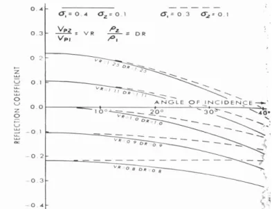
The work of Koefoed (1955) is of particular interest since his calculations involved a change in Poisson‟s ratio across the reflecting interface. He found that by having substantially different Poisson‟s ratio for the two bounding media, large change in P-wave reflection coefficients versus angle of incidence could result. Koefoed showed that under certain circumstances, reflection coefficients could increase substantially with increasing angle of incidence. This increase occurs well within the critical angle where high-amplitude, wide-angle reflections are known to occur. Figures 4 and 5 illustrate an extension of Koefoed‟s initial computations. Figure 3 shows P-wave reflection coefficients from an interface, with the incident medium having a higher Poisson‟s ratio than the underlying medium. The solid curves represent a contrast in Poisson‟s ratio of 0.4 to 0.1, while the dashed curves represent a contrast of 0.3 to 0.1. It can be deduced from the curves that Poisson‟s ratio decreases towards the underlying medium, the reflection coefficient decreases algebraically with increasing angle of incidence. This means positive reflection
23
coefficients may reverse polarity and negative reflection coefficients increase in magnitude (absolute value) with increasing angle of incidence (Ostrander 1984).
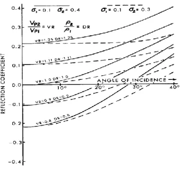
Figure 5 shows the opposite situation to that shown in Figure 4. Here Poisson‟s ratio increases going from the incident medium into the underlying medium. In this case, the reflection coefficient increases algebraically with increasing angle of incidence. Negative reflection coefficients may reverse polarity, and positive reflection coefficients increase in magnitude with increasing angle of incidence. The foregoing three illustrations point to a strong need for more information on Poisson‟s ratio for the various rock types encountered in seismic exploration. This is particularly important when one considers the long offsets commonly in use today and the resulting large angles of incidence. More information on computations of reflection and transmission coefficients can be found in Koefoed (1962) and (Tooley et al. 1965).
Fig 4. Plot of P-wave reflection coefficient versus angle of incidence for a reduction in Poisson‟s ratios across an interface (Ostrander 1984).
24
Fig 5. Plot of P-wave reflection coefficient versus angle of incidence for a increase in Poisson‟s ratios across an interface (Ostrander 1984).
2.4 APPROXIMATION TO THE KNOTT AND ZOEPPRITZ EQUATIONS
The unwieldy nature of Knott-Zoeppritz equations defies the physical insight, which forms the visualization of how the variation of a particular parameter will affect the reflection coefficient curve. Approximations are extremely useful for practical applications as they readily brings out the information in the amplitude behavior, which do not require computer to evaluate and provide the basis for certain AVO processing techniques (Castagna et al, 1993).
2.4.1 LINEAR APPROXIMATION OF ZOEPPRITZ’S EQUATION.
Zoeppritz‟s equation are implicitly coupled to the various rock properties of interest and do not provide any direct interpretive insight to the AVO behavior. For this reason, linear approximation of Zoeppritz‟s equation were developed to explicitly relate rock properties
25
thereby providing interpreters with a more direct understanding of AVO anomalies(Wardhana, 2001).
In 1961, Bortfeld linearized the Zoeppritz equations by assuming small changes in layer properties and obtained
1 2 1 2 2 2 2 1 2 1 1 2 1 1 1 2 2 1 2 sin cos cos 2 1 s s s s p p p pp V V In p In V V V V V In R
... (13)In 1976, Richards and Fraiser also followed the same approach and Aki and Richards also followed suite in 1980. They derived a form simply parameterized in terms of the changes in density, P-wave velocity, and S-wave velocity across the interface.
2.4.2 REFLECTION COEFFIECIENT BASED ON ZOEPPRITZ’S EQUATION.
In this section, an introduction of a formula of reflection coefficient developed by Zoeppritz in 1999 is illustrated. This is usually used in computing the AVO response from channel models. Consider a plane wave travelling into the earth with an angle θ, that is incident onto an interface separating two different rocks having properties (α1, β1, ρ1 and α2, β2, ρ2), and is then recorded by a receiver on the earth‟s surface in Fig 6 ( Wardhana, 2001).
26
Fig. 6 The seismic experiment (Wardhana, 2001).
The mathematical expression for the reflection of down going P and up going P waves derived by Cerveny and Ravindra in 1971 is given below.
2 3 4
2 2 4 2 1 2 1 2 2 2 2 1 1 2 1 PD P X P q PPP RCpp
... (14) Where
1 2 3 4, 2 2 3 2 2 1 4 1 2 1 2 1 2 4 3 1 1 2 2 1 2 2 2 2 2 1 2 1 Z PPX PPY PP PP q PPPP D .... (15) And
2 1 1 2 2 22
q
... (16)27 , 2 2 q X , 2 1 q Y , 2 1 2 q Z 1 1 / sin v 1 1
vv
2
1, , 2 3
v , 2 4 v 2 1 2 2 ) 1 ( i i v P
i1,2,3,4
The importance of the formulation above is that it closely fits Zoeppritz‟s equations. The only disadvantage of this long mathematical expression is that one can hardly understand the direct impact on rock-properties on reflection coefficients (Wardhana, 2001).
2.5 CONSTITUTIVE RELATIONS OF A POROUS MEDIA
Multiphase porous media embedded with a phase-change constituent have been found in numerous engineering applications, e.g., binary alloy solidification, self-healing composites, adaptive energy-absorbing foams, freeze-thaw soils, sea ice, and musculoskeletal and skin tissues. These material, typically characterized by multiphase, multi-length scales, complicated microstructure evolution process and phase-change mechanisms, are classified as “porous media”. Poroelasticity theory pioneered and developed by Terzaghi (1923, 1925) and Biot (1935, 1941, 1955, and 1962) has been used to find mechanics solutions for various porous media. The poroelasticity theory has been used to obtain analytical solutions and computational schemes including finite element and boundary element solutions to problems related to soil consolidation (Lewis and Schrefler, 1987), offshore geotechnique (Madsen, 1978; Cheng and Liu, 1986), hydraulic fracturing for energy resource exploration (Detournay and Cheng, 1991) and estimation of subsidence due to fluid withdrawal or have due to fluid injection (Verruijt, 1969). The theory has also found extensive applications in biomechanics of soft tissues and cells, mechanics of bone, transport of multiphase fluids in porous media, especially in environmental geomechanics and energy resource recovery, earthquake, and in the study of advanced materials
28
such as saturated micro-cellular foams, polymer composites, and smart materials. The applications have resulted in the modification of classical poroelasticity theory to include more complex phenomena in the description of both the porous skeleton and the interstitial fluid (Zhang, 2008).
The formulation of the constitutive equations for porous media in poroelasticity theory is based on linear elasticity and on macroscopic scale without explicitly including the contributions from solid skeleton and fluid constituents. The local portions of each constituent of the media are counted by the measure of volume fractions and the degree of saturation. It is thus essential to use micro-mechanics in obtaining the constitutive relation of multiphase porous media involving phase-change process to elicit the dependence of the bulk material coefficients on the mechanical properties and structures of each constituent at microscopic scale (Zhang, 2008).
2.6 CONSTITUTIVE RELATION
The macroscopic stresses of the multiphase porous media are calculated from the microscopic stresses using homogenization scheme, which is a volume average of the microscopic stresses within the representative unit cell and are given by
dv
V
ij
v ij
1
... (17)The macroscopic strain for porous solids is calculated by the following equation which is given by Bishop and Hill (1951).
29
u
n
u
n
ds
s
V
dv
V
ij
voids i j j i v ij
2
1
1
... (18)Where ni is the unit outward normal vector of the surfaces (Zhang, 2008).
2.7 GASSMAN FLUID SUBSTITUTION
The mechanics of fluid substitution is an important part of the seismic rock physics analysis (e.g., AVO, 4D analysis), which provides a tool for fluid identification and quantification in reservoir. This is commonly performed using Gassmann‟s equation (Gassmann, 1951). Other authors like (Batzle and Wang, 1992; Berryman, 1999; Wang, 2001; Smith et al., 2003; Russell et al., 2003; Han and Batzle. 2004) have discussed the formulations, strength and limitations of the Gassmann fluid substitution. However detailed discussions on this subject have not been fruitful (Kummar, 2006).
The objective of Gassmann‟s fluid substitution is to model the seismic properties(seismic velocities) and density of a reservoir at a given reservoir condition(e.g., pressure, temperature, porosity, mineral type and water salinity) and pore fluid saturation such as 100% water saturation or hydrocarbon with only oil or only gas saturation. Seismic velocity of an isotropic material can be estimated using known rock moduli and density. P-and S-wave velocities in isotropic media are estimated as,
3 4 K Vp ... (19) And30
sV
... (20) Respectively, where Vpand Vs are the P-and S-wave velocity, K and
are the bulk andshear moduli, and
is the mass density. Density of saturated rock can be simply computed with the volume averaging equation (mass balance). Other parameters required to estimate seismic velocities after fluid substitution are the moduli and, which can be computed using the Gassmann‟s equations (Kumar, 2006).2.7.1 GASSMANN’S EQUATIONS
Gassman‟s equations relate the bulk modulus of a rock to its pore, frame and fluid properties. The bulk modulus of a saturated rock is given by the low frequency Gassmann theory (Gassman, 1951) as
2 1 1 matrix frame matrix fl matrix frame frame sat K K K K K K K K
... (21) Where, K fra me, Kma trix , K fl are the bulk moduli of the saturated rock, porous
rock frame ( drained of any pore-filling porosity (as fraction). In the Gassmann formulation shear modulus is independent of the pore fluid and held constant during the fluid substitutions. Bulk
modulus
Ksa t
and shear modulus
at in-situ (or initial) condition can beestimated from the wireline log data ( seismic velocities and density) by rewriting equations 1 and 2 as
31
2 23
4
s p sa tr
V
V
K
... (22) And 2 sV
... (23)To estimate the saturated bulk modulus (equation 22) at a given reservoir condition and fluid type we need to estimate bulk moduli of frame, matrix and pore fluid (Kumar, 2006).
2.7.2 FLUID PROPERTIES
Bulk modulus and density of the pore fluid (brine, oil and gas) are estimated by averaging the values of individual fluid type. Let‟s first consider properties of each fluid type (brine, gas, and oil)
i) Bulk modulus and density of brine
The seismic velocity and density of brine can be used to estimate it‟s Bulk modulus.
i.e. 6 2
10
b rin e b rin e b rin eV
K
... (24)Where Kb rin eGPa, ( / )
3 cm g
b rin e
and Vb rin em/ sare the bulk modulus, density and P-wave velocity in brine. Units are given in the brackets. Brine composition can range from almost pure water to saturated saline solution (characterized by the salinity). Density and velocity in brine can be calculated following Batze and Wang (1992). Density of brine is given by
32 brine 0.668S 0.44S 10 S
300P 2400PS T
80 3T 3300S 13P 47PS
6 2 ... (25)Where PMPa and TCare the in-situ pressure and temperatures, S (as
weight fraction) is the salinity of brine, (g / cm3) is density of water given by
2 3 2 5 3 2 2
6 002 . 0 333 . 0 10 3 . 1 016 . 0 2 489 00175 . 0 3 . 3 80 10 1 T T T P TP T P T P P TP ... (26)P-wave velocity of brine, Vb rin e
m/ s
is given as
2 5 3 2
1.5
2
2 1820 16 . 0 10 780 0476 . 0 0029 . 0 6 . 2 10 5 . 8 055 . 0 6 . 9 1170 T T T P TP P S P P S S V Vbrine ... (27)Where V
m/ s
is P-wave velocity in pure water. This can be estimated by1 4 1 1 5 1
j j i ij i P T V
... (28) Where
ij constants.ii) BULK MODULUS AND DENSITY OF GAS
Bulk modulus and density of a gas in a reservoir depend on the pressure, temperature and the type of gas, Hydrocarbon gas can be a mixture of many gases, and they are characterized by specific gravity G, the ratio of the gas density to air density of
c
6 . 15
and atmospheric pressure. Following Batzle and Wang (1992) density of gas can be estimated as
( 273.15) 8 . 28 T ZR GP g a s
... (29)33
Where G is the specific gravity of gas (API), R is the gas constant (8.314) and Z is the compressibility factor given by:
T
P
T
T
E
Z
0
.
03
0
.
00527
(
3
.
5
pr)
3 pr
0
.
642
pr
0
.
007
pr4
0
.
52
... (30) And
pr pr pr pr T P T T E 2 . 1 2 2exp 0.45 80.56 1/ ) 85 . 3 ( 109 . 0 ... (31)In the above equation, Tp r and Pp r are the pseudo-reduced temperature and
pressure, respectively, and are given by
G T Tp r 75 . 170 72 . 94 15 . 273 ... (32)
The bulk modulus of gas (GPa) is given by (Batzle and Wang, 1992)
1000 1 T p r p r g a s P Z Z P P K ... (33)
iii) BULK MODULUS AND DENSITY OF OIL
Oil contains some dissolved gas characterized by the GOR (gas-to-oil ratio) value. Similar to gas, oil, density and bulk modulus depend on the temperature, pressure, GOR and the type of oil. Density and velocity in oil can be written following Batzle and Wang (1992) and Wang (2001) as,
34
175 . 1 4 4 2 3 7 ) 78 . 17 ( 10 81 . 3 972 . 0 10 49 . 3 15 . 1 10 71 . 1 00277 . 0 T P P P s s oil ... (34) And TP P T V ps ps ps oil 3.7 4.64 0.0115 18.33 16.97 1 6 . 2 2096 ... (35)Where o il
g / cm3
and Vo ilm/ s are the density and P-wave velocity in oil (containing some dissolved gas). In the above equations,s
and
p s are the saturation density and pseudo density given as
B G RG s 0012 . 0 ... (36) And
1 0.001RG
B0 p s
... (37)Where RG is the GOR (litre/litre),
3
/ cm
g
is the reference
density of oil measured at 15.6oC and atmospheric pressure and is called the formation volume factor which is given by the formula
35 1 7 5 . 1 8 . 17 495 . 2 00038 . 0 972 . 0 R G T B G ... (38) Once velocity and density are known, bulk modulus of oil, Ko il(GPa)can be calculated as 6 2 10 o il o il o il V K
... (39)Fluid in the pore spaces consists of brine and hydrocarbon (oil and /or gas). Bulk modulus and density of the mixed pore fluid phase can be estimated by inverse bulk modulus averaging (also known as Wood‟s equation) and arithmetic averaging of densities (i.e., mass balance) of the separate fluid phases, respectively. Bulk modulus
K fl and density
fl of the fluid phase are given asfl b rin e Kh yc HS K WS K 1 ... (40) And
fl
WS
b rin e
HS
h yc ... (41) Where WS is the water saturation (as fraction) and HS (= 1 –WS) is the hydrocarbonsaturation, Kh yc and h ycare the bulk modulus and density of hydrocarbon, respectively, In the case of oil as hydrocarbon,
36
K
h yc
K
o il ... (42) And
h yc
o il ... (43)And in the case of gas as hydrocarbon,
K
h yc
K
g a s ... (44) And
h yc
g a s ... (45)2.7.3 FRAME PROPERTIES
Frame bulk modulus can be derived from the laboratory measurement, empirical relationship, or
wireline log data. When working with wire line data, K fra mecan be determined by
rewriting the Gassmann equation (equation 20) for K fra me(Zhu and McMechan, 1990) as
1 1 ma trix sa t fl ma trix ma trix fl ma trix sa t fra me K K K K K K K K K ... (46)
37
All the parameters in the above equation (36) are known from the previous
formulation: Ksa t(equation4), Kma trix(equation6), )
30 (equation
K fl . The
fr a me
K value remains unchanged during
fluid substitution.
2.7.4 MATRIX PROPERTIES
To calculate the bulk modulus of mineral matrix, one needs to know the mineral composition of rock. This can be found from laboratory examination of core samples. Litho logy can be assumed to be a composition of quartz and clay minerals in the absence of laboratory data. The percentage of clay can be derived from the volume shale (Vsh) curve, which is typically derived from the wire log data (Gamma-ray log). Typical shale contains about 70% of clay and 30% of other minerals (mostly quartz). Once the mineral abundances are determined, Kmatrix can be calculated via the application of Voigt-Reuss-Hill (VRH) averaging (Hill, 1952) of the mineral constituents. Input for Kmatrix calculation are Vsh, Kclay (bulk modulus of clay), Kqtz (bulk modulus of quartz). The Kmatrix can be calculated by the VRH averaging as
qtz qtz clay clay qtz clay clay matrixK
V
K
V
V
K
V
K
2
1
... (47)Where Vclay and Vqtz are
38 And
Vqtz = 1- Vclay
Density of the mineral matrix
ma trixcan be estimated by arithmetic averaging of densities of individual minerals as qtz atz clay clay matrixV
V
Where
cla y and
q tzare the density of the clay and quartz minerals. Bulk moduli of clay (20.9GPa) and quartz (36.6Gpa), and densities of clay (2.58g/cm3) and quartz (2.65 g/cm3) can be found in text books (e.g., Mavko, Mukerji and Dvorkin, 1998) or from the core analysis in thelaboratory. The values of Kmatrix and
ma trixremain constant during the Gassman fluid substitution.39 CHAPTER 3
METHODOLOGY
3.1 INTRODUCTION
The science of seismology began with the study of naturally occurring earthquakes. Seismologists at first were motivated by the desire to understand the destructive nature of large earthquakes. They soon learned however that the seismic waves produced by an earthquake contained valuable information about the large-scale structures of the Earth interior. Today, a much of our understanding of the Earth mantle crust and core is based on the analysis of the seismic waves produced by earthquakes. Thus seismology became an important branch of geophysics, which is the physics of the Earth (Brian, 1997).
Seismologists and geologists also discovered that similar but much weaker man-made seismic waves had a more practical use. They could probe the very shallow structure of the Earth to help locate its mineral water and hydrocarbon resources, thus the seismic exploration industry was born and the seismologists working in that industry came to be called exploration geophysicist. Today seismic exploration encompasses more than just the search for resources. Seismic technology is used in the search for waste-disposal sites in determining the stability of the ground under proposed industrial facilities and even in archaeological investigations. Nevertheless, since hydrocarbon exploration is still the reason for the existence of the seismic exploration industry, the methods and terminology explained related to seismic are commonly used in the oil and natural gas exploration industry. The underlying concept of seismic exploration is simple Man-made seismic waves are just waves (also called acoustic waves) with
40
frequencies typically ranging from about 5Hz to just over 100Hz. ( The lowest sound frequency audible to the human ear is about 30Hz). As these sound waves leave the seismic source and travel downward into the Earth, they encounter changes in the Earths geological layering which cause echoes ( or reflections) to travel upward to the surface Electromechanical transducers ( geophones or hydrophones) detect the echoes arriving at the surface and convert them into electrical signals which are then amplified, filtered, digitized an recorded. The recorded seismic data usually undergo elaborate processing by digital computers to produce images of the earth‟s shallow structure. An experienced geologist or geophysicist can interpret those images to determine what type of rocks they represent and whether those rocks might contain valuable resources (Brian, 1997).
It is commonly assumed that a stacked seismic trace is the convolution of a wavelet and a vertical incidence reflection coefficient series. In reality seismic energy in a shot record strikes any given boundary with a wide range of incidence angles resulting in P to S wave conversion. It is easily shown in the resulting reflection coefficient depends on P-wave velocity, S-wave velocity and layer density and the variation of P-wave reflected amplitude with angle of incidence (or offset) depends on Poisson‟s ratio and density contrasts between layers. Various authors including shuey (1985) have published simplified approximations of the full Zoeppritz equations. The AVO response equation at a boundary between two layers is commonly expressed as:
2 2 2sin
1
/
cos
)
(
R
R
... (48)41
Where R (θ) is the reflection coefficient at angle of incidence θ, σ is Poisson‟s ratio and Ro is the
reflection coefficient at zero offset.
Note that this two term equation is valid only up to 30 degrees angle of incidence. The two terms tell us that the AVO response is dominated by Ro at small angles and the contrast in Poisson‟s ratio at large angles. The equation also tells us that an increase in Poisson‟s ratio across the boundary will cause an increase in reflected amplitude with angle of incidence and vice versa. So intuitively, an interface may show a positive, negative or zero Ro, and the amplitude may either increase or decrease with offset. This leads so far, to six potential observations on a seismic gather (McGregor, 2007).
High amplitude reflections associated with the boundary between gas-bearing zones (sands) and cap rocks (shale) are routinely referred to as “bright spots” (Khattri et al, 1979). Offset dependent reflection amplitude (Amplitude Versus Offset [AVO] characteristics for gas rich sediments can vary significantly with geologic setting, gas concentrations, and lithology (Ostrander, 1982). Three unique types of reservoirs or classes of gas deposits have been described that incorporate geology setting and lithology with seismic attributes (Rutherford and Williams, 1989). Lithologically, the encasing medium or mechanism and reservoir rock distinguish these classes while seismically, a distinct impedance range aids in classifying each type of gas sand (Begay et al, 2000).
3.2 WHAT ARE SEISMIC DATA
Seismic data is generated by using vibrations to capture a two-dimensional picture of the rock layers beneath the surface. The interpretation of seismic data allows the scientist to make an
42
estimated picture of the rocks beneath the surface without drilling or digging trenches. The collection of vibrations which, when coupled with time elements, represent the rate of transmission of energy through a material. Scientist have measured many different materials and have a portfolio of data which allow them to interpret the type of material, the structure of the material, and the depth below the surface of the material, all based upon the nature of the vibrations. The data are used in many ways, from determining how thick the soil may be in an area, to locating cracks in the rocks.
3.2.1 BACKGROUND OF THE INVENTION
Seismic surveys are conducted for the purpose of investigating and modeling the depth and structure of subsurface earth formations as a preliminary activity in exploiting natural resources. During the course of reflection seismometry, a source, emplaced at or near the surface of the earth, radiates an acoustic wavefield. The wavefield may be created by an impulsive source, by a chirp-signal generator or any other means now known or unknown. The wavefield propagates downwardly into the earth to insonify the earth strata below. The wavefield is reflected from the respective subsurface strata back to the surface where the mechanical motions of the seismic waves are converted to electrical signals by seismic sensors such as geophones or accelerometers. The received, reflected seismic signals may be recorded and processed by means well known to the art such as by computer, to provide and display a multi-dimensional model. Seismic studies may be performed in one dimension to provide a single time-scale trace exhibiting a desired seismic parameter as a simple function of time ( or depth if the propagation velocity of seismic waves is known). The data are generated using a substantially single source
43
and a substantially single sensor which may be, for example lowered to various levels in a borehole as in vertical seismic profiling (VSP) (Lapucha, 1994).
Seismic surveys may be conducted in two dimensions (2-D) wherein a plurality of sensors, such as for example, 100 are distributed at spaced-apart interval, commonly known to the industry as a spread, along a designated line of survey at or near the surface of the earth. Each sensor or compact group of several interconnected sensors is coupled by a signal transmission means to a dedicated signal-conditioning and recording channel. Seismic sensors receive the wavefield after reflection from the earth formations below. The electrical signals resulting from the reflected waveforms may be recorded, processed and formatted as a plurality of time-scale traces. The time-scale traces provide an analog of a cross section of the earth along a single vertical plane having the dimensions of reflection travel time vertically, and offset distance horizontally. After each shot, source and sensors are progressively advanced along the line of survey by a preselect incremental distance until the entire length of the survey line has been occupied (Lapucha, 1994).
Three dimensional (3-D) surveys may be conducted wherein many hundreds or thousands of seismic sensors are distributed aerially over an extended region in a grid pattern of sensor stations established with reference to north and east geographic coordinates. Typical grid dimensions might be on the order of 50 by 100 meters. A 3-D survey is capable of providing a model of a volumetric cube of the sub-surface earth strata. Each sensor or sensor group is connected to a single recording channel. Each time that a source is fired, it insonifes a large patch of sensors. After each firing, the source moves to a new location where the firing is repeated. Three dimensional data acquisition systems depend upon real-time transmission of the seismic data through a multi-channel telemetric system. All of the data are recorded and partially