2 Sismantilles I experiment and a-priori location
2.1 Network Layout and quality of earthquake data
In well instrumented subduction zones like the Japan arc, locations of earthquakes under the offshore forearc and the interplate megathrust seismogenic zone have been demonstrated to be grossly in error, once they obtained records of Ocean Bottom Seismometers (hereafter OBS) deployed far offshore (Hasegawa et al., 1991). Offshore Tohoku, the first OBS deployment for long-term earthquake observation had started in 1987 and continued to present with 3 permanent sensor sites cabled to the coast.
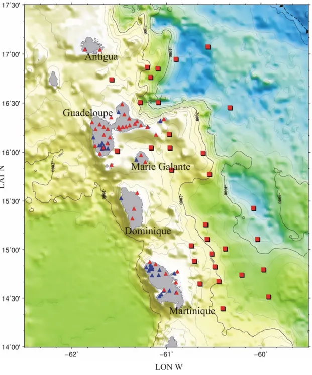
In the Lesser Antilles, between November 1999 and January 2002, a temporary field experiment, conducted by « Laboratoire de sismologie expérimentale » of the « Institut de Physique du Globe de Paris » (hereafter IPGP), has been carried out over a large region along the arc between the Martinique and Antigua islands (figure 2.1). This experiment, named SISMANTILLES I, represents the first successful attempt of a combined on-offshore seismological network in this area and was aimed to record local earthquake activity and to provide a data-set which would allow high precision earthquake location and permit the inversion for one- and three-dimensional crustal velocity structure. Several authors (see paragraph 1.3) provide information about the distribution of the seismicity in the region, these information were used to plan a temporary seismic network that complemented a local seismic network from the « Observatoire Volcanologique et Sismologique de Guadeloupe» (hereafter OVSG). 39 one-component stations equipped primarily with short period seismometers having a natural frequency of 1 Hz composed this seismic array. The seismic network of the SISMANTILLES I experiment, that covered an area of about 150 km in NEE-SWW direction and of about 300 km in NNW-SSE direction, it was composed of two parts: a landward and a seaward network, which will be described separately in the following.
The landward network was formed by 43 three components seismic stations from IPGP that operated from November 1999 to August 2000 and for a second period from November 2001 to January 2002. The deployment of IPGP seismic stations (red triangles in figure 2.1) led to an homogeneous distribution of network components, avoiding a concentration on the flanks of “La Soufrière” and “Montagne Pelée” volcanoes. With this addition, the seismic network was optimized in order to locate regional seismic events.
Figure 2.1: Map showing OBS and land stations used in SISMANTILLES I experiment. Blue triangles: seismic stations of OVSG. Red triangles: temporary seismic stations. Red squares: off-shore network. Bathymetry is from Smith and Sandwell (1997). The deformation front, related to the subduction of the Atlantic Ocean lithosphere beneath the Caribbean Plate, is represented by dashed line with triangles.
These temporary seismic stations were equipped with three types of recording instruments: Mini Titan HI7190, Reftek model 130-02, and Hathor3. All instruments, recording on a continuously mode with a sampling rate of 100 Hz, were equipped with a 5s (Titan and Rftek) or a 2 Hz three-component seismometer.
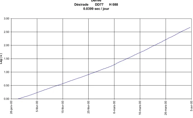
During the fieldwork station coordinates were taken with the GPS instruments with errors in latitude and longitude inferior to ± 10 m. Analysis of earthquake data also requires that the correct time for each data point on a seismic trace (sample) is known with certain accuracy. Indeed the kind of analysis, which can be successfully undertaken, and its quality are strongly coupled with this accuracy. In the Titan and Reftek stations the true time derive directly from GPS satellite, the seimic signal is either saved on the data records directly or used to control and update an internal clock in the recording unit which is then used to set the time on the data.On the contrary, in the Hathor stations the internal clock is not corrected with the external pulse; only the difference between internal and external time (lag) is recorded together with the internal time. The lag (figure 2.2) is then applied to correct the internal time when processing data.
Figure 2.2: Lag value for the Desirade station in the period 26-01-2000/05-04-2000.
Dérive Désirade DD77 H 088 0.0399 sec / jour 0.00 0.50 1.00 1.50 2.00 2.50 3.00 2 6 -ja n v-0 0 5 -f év r-00 1 5-fé vr -0 0 25 -f év r-00 6-m ar s-00 1 6 -m a rs -0 0 2 6-m ar s-00 5 -a vr -0 0 L a g ( s )
After a failed attempt due to ship breakdown, the landward network has been complemented by 31 OBS. These instruments were left on the seafloor for 69 days starting November 24th, 2001 to record simultaneously natural seismicity and the MCS shots from the
french N/O Nadir vessel (Laigle et al., 2005).
To better locate the interplate seismicity, it was particularly important to have records of OBS located directly above the hypocentres. Indeed land stations were too far from the sources and do not allow to obtain earthquake locations with good azimuthal coverage. As observed on most of the ocean-floor observatories, the noise level at the OBS site is quite large on all components (Dahm et al., 2006). However, although a higher noise level yield gives a lower sensitivity for OBS’s, one or more observations improve the azimuthal coverage and constrain a better hypocenter location. The OBS use, as in this case, is limited by their low battery life (approximately 8 weeks for continuous recording).
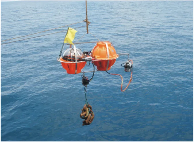
All OBS (figure 2.3) stations were equipped with a three-component seismometer, 9 of them (from the Institut de recherche pour le développement of Villefranche-sur-Mer - France) are characterized by short period 4.5 Hz seismometers and 22 (from the Institute of Seismology and Volcanology of Okkaido - Japan) by broadband seismometers (60s). They recorded on a continuous mode at sampling rate of 100 Hz. A linear time drift correction was applied to the data taking into account time synchronized with GPS clock just before the deployment and just after recovery of the OBS. In total 140 instruments, all running in continuous mode, were in use. All station positions used in the SISMANTILLES I experiment are shown in figure 2.1.
2.2 Determination of first arrival times
Identifying first arrival times of P- and S- waves on waveforms was done with Pickev software for Reftek and Hathor data (Fréchet et Thouvenot, 2000), with Rtoo software (elaborated by A. Nercessian of IPGP) for Titan and OBS data. To the arrival time readings of the IPGP temporary seismometers, the readings of the permanent array primarily composed of vertical component seismometer could be added by courtesy of OVSG.
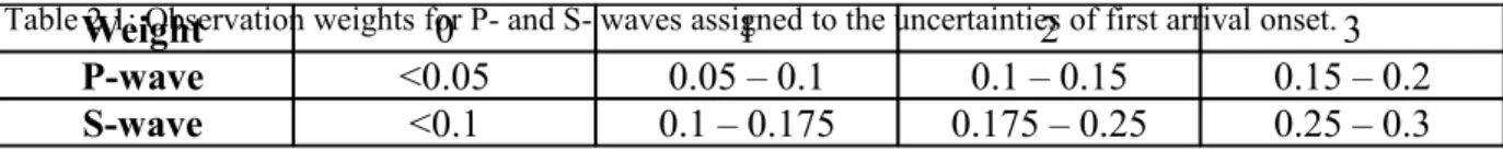
Observation weights are assigned according to the Table 2.1, for the temporary network S-wave arrivals are only picked on the horizontal components because all stations are three components.
Table 2.1: Observation weights for P- and S- waves assigned to the uncertainties of first arrival onset.Weight 0 1 2 3
P-wave <0.05 0.05 – 0.1 0.1 – 0.15 0.15 – 0.2
Most of the P wave arrivals were assigned a weight of 0 as they could be read with a picking accuracy lesser than 0.05 s.
Figure 2.3: OBS are autonomous instruments that sit seafloor and record waves. Floats made from glass balls and syntactic foam make each OBS buoyant, but an anchor holds it on the seafloor during the survey. Photo shows an OBS deployment.
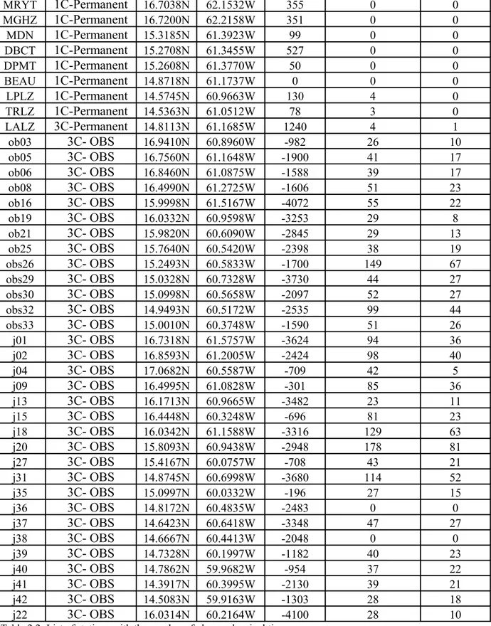
The following table gives the list of stations and the number of times they are found into the original phases file:
NAME Number of
components - Network
Latitude Longitude Altitude Total number arrivals Number S-arrivals MV3 3C-Temporary 14.5547N 60.8892W 355 79 38 ZA3 3C-Temporary 14.5845N 61.0227W 17 67 33 ROS 3C-Temporary 14.6600N 60.8963W 28 88 44 PROS 3C-Temporary 14.6600N 60.8963W 28 23 11
BONA 3C-Temporary 14.7493N 61.0043W 197 26 13 AIR 3C-Temporary 14.7493N 61.0043W 197 59 29 CAR 3C-Temporary 14.7723N 60.8817W 124 24 12 LEY 3C-Temporary 14.8468N 61.1123W 136 33 16 BSJ 3C-Temporary 14.8718N 61.1737W 135 29 14 OPH 3C-Temporary 15.3148N 61.3590W 107 62 28 PEN 3C-Temporary 15.4148N 61.3417W 304 176 81 WES 3C-Temporary 15.5775N 61.3077W 40 193 88 SAIN 3C-Temporary 15.8647N 61.5795W 0 118 59 PERE 3C-Temporary 15.8938N 61.2227W 24 185 89 GRE 3C-Temporary 15.9655N 61.2678W 70 173 84 OBS 3C-Temporary 15.9798N 61.7032W 408 125 56 GALI 3C-Temporary 16.0387N 61.6645W 1140 25 10 GDE 3C-Temporary 16.0565N 61.7528W 55 30 15 BRI 3C-Temporary 16.0823N 61.6237W 432 205 102 DOUV 3C-Temporary 16.1438N 61.5967W 100 151 74 PTT 3C-Temporary 16.1707N 61.1093W 8 43 21 VERN 3C-Temporary 16.1713N 61.6602W 221 117 55 ESPE 3C-Temporary 16.2295N 61.7480W 148 316 157 RETR 3C-Temporary 16.2307N 61.6197W 44 142 70 BARB 3C-Temporary 16.2323N 61.4942W 70 411 196 CHA 3C-Temporary 16.2503N 61.2007W 9 63 25 TER 3C-Temporary 16.2505N 61.5037W 43 34 17 TASS 3C-Temporary 16.2512N 61.4622W 63 296 142 DONO 3C-Temporary 16.2518N 61.6615W 55 6 3 ZABR 3C-Temporary 16.2550N 61.4257W 109 158 78 LOU 3C-Temporary 16.2667N 61.3878W 36 147 69 AERO 3C-Temporary 16.2673N 61.2688W 31 45 21 BIS 3C-Temporary 16.2772N 61.7047W 130 209 95 CELC 3C-Temporary 16.2847N 61.3318W 34 287 130 NTRD 3C-Temporary 16.2993N 61.7857W 148 201 98 BLMA 3C-Temporary 16.3092N 61.3093W 31 204 92 DESI 3C-Temporary 16.3317N 61.0250W 177 262 127 NERO 3C-Temporary 16.3367N 61.3932W 48 180 85 FAJ 3C-Temporary 16.3500N 61.5833W 0 152 75 DANJ 3C-Temporary 16.3798N 61.4442W 4 268 128 HYP 3C-Temporary 16.4840N 61.4672W 33 227 98 FRE 3C-Temporary 17.0412N 61.7023W 82 319 158 BOG 3C-Temporary 17.0450N 61.8613W 367 335 155 BIMZ 1C-Permanent 14.5170N 61.0708W 425 356 126 MBIG 1C-Permanent 14.5170N 61.0708W 425 24 12 TRMZ 1C-Permanent 14.5363N 61.0512W 78 249 58 MVMZ 1C-Permanent 14.5545N 60.8955W 361 316 92 ZAMZ 1C-Permanent 14.5727N 61.0287W 25 360 111 LPMZ 1C-Permanent 14.5745N 60.9663W 130 325 83 FDFZ 3C-Permanent 14.7333N 61.1503W 510 472 213 BVMZ 1C-Permanent 14.7350N 61.0797W 694 291 75 CRMZ 1C-Permanent 14.7537N 60.9155W 180 307 94
MLMZ 1C-Permanent 14.7810N 61.1838W 370 251 45 MJMZ 1C-Permanent 14.7887N 61.0708W 400 52 18 PCMZ 1C-Permanent 14.7968N 61.1487W 730 211 47 GBMZ 1C-Permanent 14.7973N 61.1648W 800 357 107 LAMZ 3C-Permanent 14.8113N 61.1685W 1240 303 107 CPMZ 1C-Permanent 14.8155N 61.2105W 335 341 90 BAMZ 1C-Permanent 14.8157N 61.1483W 670 391 125 SAMZ 1C-Permanent 14.8417N 61.1678W 510 122 22 BBLZ 1C-Permanent 15.5230N 61.4780W 365 91 5 MGGZ 1C-Permanent 15.9180N 61.3168W 51 135 1 PAGZ 1C-Permanent 16.0297N 61.6800W 670 173 37 DOGZ 1C-Permanent 16.0320N 61.6178W 460 193 1 LKGZ 1C-Permanent 16.0328N 61.6583W 1380 69 7 ECGZ 1C-Permanent 16.0400N 61.6572W 1406 42 0 TAGZ 1C-Permanent 16.0420N 61.6642W 1182 316 113 RMGZ 1C-Permanent 16.0443N 61.6657W 1150 70 0 CAGZ 1C-Permanent 16.0542N 61.6592W 1370 139 3 FNGZ 1C-Permanent 16.0603N 61.6867W 825 199 1 MOGZ 1C-Permanent 16.0613N 61.7103W 640 147 4 BRGZ 1C-Permanent 16.0850N 61.6197W 442 140 2 STGZ 1C-Permanent 16.0887N 61.6788W 1210 6 1 LZGZ 1C-Permanent 16.1430N 61.7720W 97 156 3 SFGZ 1C-Permanent 16.2533N 61.1965W 10 35 0 MONT 1C-Permanent 16.3112N 61.0638W 303 53 26 DEGZ 1C-Permanent 16.3132N 61.0618W 275 520 218 SEGZ 1C-Permanent 16.4028N 61.5052W 60 147 2 BPAZ 1C-Permanent 17.0460N 61.8570W 396 15 1 SLBZ 1C-Permanent 13.8258N 61.0408W 600 0 0 OBSZ 1C-Permanent 14.7333N 61.1503W 510 0 0 PAMZ 1C-Permanent 14.6138N 61.0363W 120 0 0 ABGZ 1C-Permanent 16.0323N 61.6603W 1150 0 0 EGCZ 1C-Permanent 16.0302N 61.6538W 1395 0 0 FBGZ 1C-Permanent 15.9678N 61.6487W 185 0 0 HMGZ 1C-Permanent 15.9707N 61.7000W 420 2 1 MLGT 1C-Permanent 16.7250N 62.1623W 287 0 0 MLGZ 1C-Permanent 16.7250N 62.1623W 287 83 5 MSGZ 1C-Permanent 16.0987N 61.7220W 851 0 0 PRGZ 1C-Permanent 16.0362N 61.6622W 1070 0 0 MDNZ 1C-Permanent 15.3160N 61.4000W 99 0 0 NEVZ 1C-Permanent 17.1360N 62.5710W 244 0 0 SLWZ 1C-Permanent 14.0200N 60.9360W 366 29 8 CHAZ 1C-Permanent 13.8583N 61.0643W 242 0 0 MCAZ 1C-Permanent 13.8503N 61.0190W 615 0 0 MSPT 1C-Permanent 16.6910N 62.2000W 106 0 0 H5BZ 1C-Permanent 14.4250N 60.8367W 10 20 8 H5AZ 1C-Permanent 16.3133N 61.0605W 255 1 0 CPB 1C-Permanent 17.6400N 61.8260W 5 0 0 MJHT 1C-Permanent 16.7672N 62.1697W 1870 0 0
MRYT 1C-Permanent 16.7038N 62.1532W 355 0 0 MGHZ 1C-Permanent 16.7200N 62.2158W 351 0 0 MDN 1C-Permanent 15.3185N 61.3923W 99 0 0 DBCT 1C-Permanent 15.2708N 61.3455W 527 0 0 DPMT 1C-Permanent 15.2608N 61.3770W 50 0 0 BEAU 1C-Permanent 14.8718N 61.1737W 0 0 0 LPLZ 1C-Permanent 14.5745N 60.9663W 130 4 0 TRLZ 1C-Permanent 14.5363N 61.0512W 78 3 0 LALZ 3C-Permanent 14.8113N 61.1685W 1240 4 1 ob03 3C- OBS 16.9410N 60.8960W -982 26 10 ob05 3C- OBS 16.7560N 61.1648W -1900 41 17 ob06 3C- OBS 16.8460N 61.0875W -1588 39 17 ob08 3C- OBS 16.4990N 61.2725W -1606 51 23 ob16 3C- OBS 15.9998N 61.5167W -4072 55 22 ob19 3C- OBS 16.0332N 60.9598W -3253 29 8 ob21 3C- OBS 15.9820N 60.6090W -2845 29 13 ob25 3C- OBS 15.7640N 60.5420W -2398 38 19 obs26 3C- OBS 15.2493N 60.5833W -1700 149 67 obs29 3C- OBS 15.0328N 60.7328W -3730 44 27 obs30 3C- OBS 15.0998N 60.5658W -2097 52 27 obs32 3C- OBS 14.9493N 60.5172W -2535 99 44 obs33 3C- OBS 15.0010N 60.3748W -1590 51 26 j01 3C- OBS 16.7318N 61.5757W -3624 94 36 j02 3C- OBS 16.8593N 61.2005W -2424 98 40 j04 3C- OBS 17.0682N 60.5587W -709 42 5 j09 3C- OBS 16.4995N 61.0828W -301 85 36 j13 3C- OBS 16.1713N 60.9665W -3482 23 11 j15 3C- OBS 16.4448N 60.3248W -696 81 23 j18 3C- OBS 16.0342N 61.1588W -3316 129 63 j20 3C- OBS 15.8093N 60.9438W -2948 178 81 j27 3C- OBS 15.4167N 60.0757W -708 43 21 j31 3C- OBS 14.8745N 60.6998W -3680 114 52 j35 3C- OBS 15.0997N 60.0332W -196 27 15 j36 3C- OBS 14.8172N 60.4835W -2483 0 0 j37 3C- OBS 14.6423N 60.6418W -3348 47 27 j38 3C- OBS 14.6667N 60.4413W -2048 0 0 j39 3C- OBS 14.7328N 60.1997W -1182 40 23 j40 3C- OBS 14.7862N 59.9682W -954 37 22 j41 3C- OBS 14.3917N 60.3995W -2130 39 21 j42 3C- OBS 14.5083N 59.9163W -1303 28 18 j22 3C- OBS 16.0314N 60.2164W -4100 28 10
Table 2.2: List of stations with the number of observed arrival times.
Our data base comprises about 15,500 arrival readings. The S-wave readings, read primarily on horizontal components, are about 5,700.
2.3 The a-priori velocity models
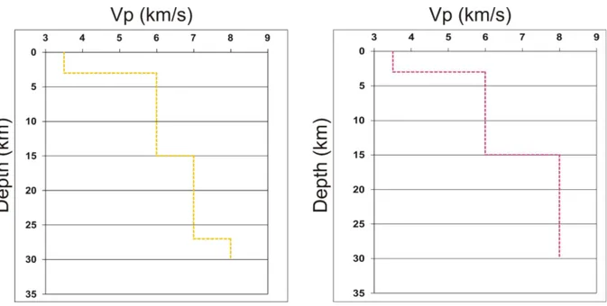
A major feature of the Lesser Antilles region is the high-gradient crustal thinning from the Caribbean island arc (~30 km) to the North American Plate (~15 km) (Roux, 2007). For this reason, we consider two 1-D a priori models derived from the studies of Dorel et al. (1974) and from seismic refraction profiles of the Ladle Study Group (1983):
Model 1 (Dorel, 1981) : 3.5 km/s (depth -3.0 3.0 km), 6.0 km/s (depth 3.0 15.0 km), 7.0 km/s (depth 15.0 30.0 km), 8.0 (depth >27.0 km)
Model 2 (Ladle Study Group, 1983): 3.5 km/s (depth -3.0 3.0 km), 6.0 km/s (depth 3.0 15.0 km), 8.0 (depth >15.0 km).
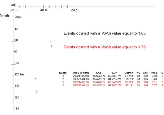
In the model 1, with regard to the Moho depth, we consider the results obtained by Kopp et al. 2011. The Vp/Vs value is very important for the hypocenter determination. An example is provided by two earthquakes with many observations occurred to the east of Dominique Island. If Vp/Vs value changes from 1.85 to 1.75 we note differences in the source depth in the order 10-20 kms for the deeper events (figure 2.5). Evidently we have a minor influence of the different Vp/Vs ratios for the determination of focal depth for the shallower events. On the basis of a recent analysis of OSVG data-base (Clément, 2001), the value of 1.76, determined via Wadati diagrams, have been chosen as initial Vp/Vs ratio.
Figure 2.4: The two a-priori 1-D velocity models used in this study. On the left Model 1 of Dorel et al. (1974). On the right the Model 2 (Ladle Study Group, 1983).
Depth 20km 40 60 80 100 120 km 140 160 180 Lon -61.5 -61.0 -60.5 1 2 1 2
Events located with a Vp/Vs value equal to 1.85
Events located with a Vp/Vs value equal to 1.75
EVENT ORIGIN TIME LAT LON DEPTH NO GAP RMS Q
1 000214 00:18 15.6258 N 60.8807 W 61.748 63 192 0.60 B
2 000505 04:43 15.4222 N 61.2204 W 125.762 70 145 0.70 B 1 000214 00:18 15.6260 N 60.8433 W 72.379 63 196 0.31 B 2 000505 04:43 15.3853 N 61.2051 W 147.121 70 146 0.37 A
Figure 2.5: E-W cross section of hypocenters computed by using the programme VELEST and the 1-D velocity model proposed by Dorel et al. (1974). These events are located with Vp/Vs value equal to 1.85 (black) and to 1.76 (red).
2.4 The use of S- wave readings in hypocenter locations
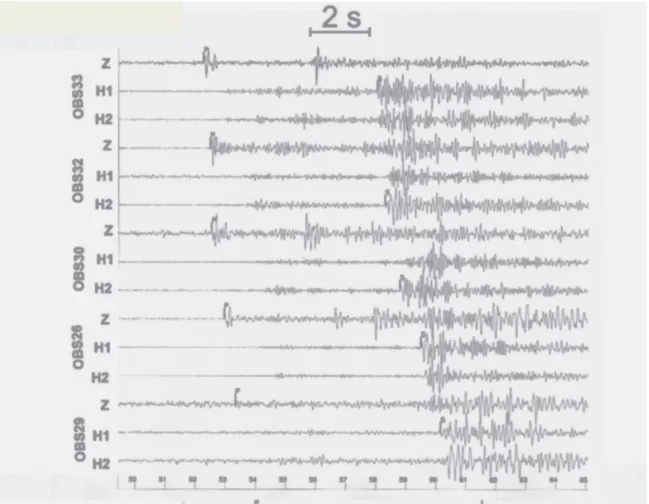
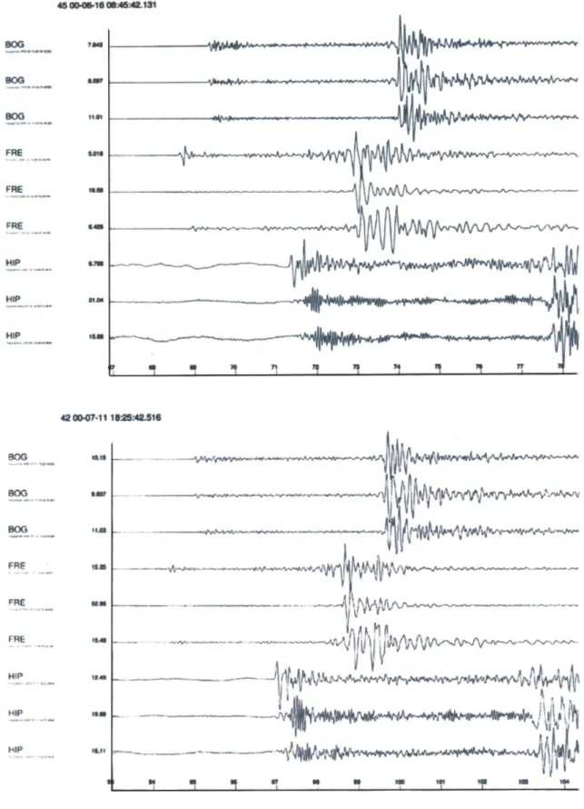
In this section we emphasize as the use of S-wave readings is very important to obtain good hypocentre locations. As figure 2.6 shows, the S-wave readings are often not possible if we dispose of only one-component seismic stations, like in the case of the OVSG permanent network.
Since the sensors of seismic arrays are currently placed at or near the topographical surface, if the horizontal aperture of the array is chosen, its vertical extension is restrained. From simple geometrical considerations, the array resolution power for source location is better for the horizontal coordinates and that on the vertical one decreases with increasing depth. However if two waves emitted simultaneously from the source propagate with different velocities, each sensor resolves the range and hypocentral depth receives an additional constraint (Hirn et al., 1991).
Figure 2.6: Typical records of an event obtained by five OBS. High quality of S-waves readings obtained thanks to the horizontal components of OBS. These events have been located at more than 40 km depth. In the absence of the horizontal components, the S waves would have been picked on the vertical sensor with an error of about 2 seconds due to the strong P to S converted waves.
An example is provided by the two earthquakes of figure 2.5 occurred to the east of Dominique Island. If only P arrivals are used we note very little differences in horizontal location but a big shift, from 10 to 35 km, of the hypocenter depth (figure 2.7). That these hypocenters are incorrect are not evident from formal errors of the VELEST output file on the hypocenter locations (Kissling, 1995), rms values in fact increase from less than 0.3 s to 0.6-0.7 s by the addition of S-wave observations. Another example is provided by a multiplet of seven events occurred between Guadeloupe and Antigua Island. A multiplet is a group of seismic events with very similar waveforms, despite different origin times (figure 2.8). Many studies assert that waves generated by similar sources, propagating along similar paths, will generate similar waveforms and likely a multiplet is the expression of stress release on the same structure (Fremont et Malone, 1987).
Figure 2.7: E-W cross section of two hypocenters computed with P- and S-wave observations (black) and with only first arrivals (red). These events are located by using the programme VELEST and the 1-D velocity model proposed by Dorel et al. (1974).
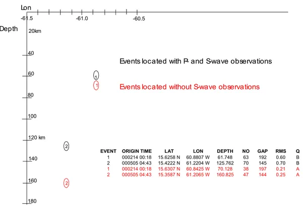
In figure 2.8 we can note a constant interval between P and S arrivals and also similar wave shapes which constrain the sources to be at a same depth and very tightly clustered. If only P arrivals are used, the events spread over a volume that is elongated by more than 10 km in depth (figure 2.9). Depth 20km 40 60 80 100 120 km 140 160 180 Lon -61.5 -61.0 -60.5 1 2 1 2
EVENT ORIGIN TIME LAT LON DEPTH NO GAP RMS Q
1 000214 00:18 15.6258 N 60.8807 W 61.748 63 192 0.60 B 2 000505 04:43 15.4222 N 61.2204 W 125.762 70 145 0.70 B
1 000214 00:18 15.6307 N 60.8425 W 70.128 38 197 0.21 A 2 000505 04:43 15.3587 N 61.2065 W 160.825 47 144 0.25 A
Events located with P- and S-wave observations Events located without S-wave observations
Figure 2.8: Two seismograms from the multiplet of seven events occurred on July 2000 between Antigua and Guadeloupe Island. Note constant interval between P and S arrivals and also similar wave shapes.
Also in this example, that the hypocenters located without –S readings are incorrect are not evident from formal errors of the output file on the hypocenter locations, rms values in fact
increase from less 0.3 s to 0.3-0.6 s by the addition of S-wave observations. Therefore we may have a more precise location only by adding good S readings.
Figure 2.9: Map location and E-W cross section of a multiplet computed with P- and S-wave observations (black) and with only first arrivals (red). These events are located by using the programme VELEST and the 1-D velocity model proposed by Dorel et al. (1974).
2.5 The earthquake selection for the 1-D inversion
Our SISMANTILLES I data base comprises almost 1,000 earthquakes with an average number of observations for event equal to 15.7. In this step, we obtain the a-priori location by using VELEST (Kissling, 1995) in single-event mode. Successively, in the second step of LET, we read, by using the same software but in simultaneous mode, the input files with the selected best events. In this step of inversion process, to assess the unknown parameters, the norm of the misfit function is minimized in a least squares sense. This means that, although this method is robust, large residuals are overweighs and are likely to bias the process. This Depth 10km 20 30 40 50 60 km 70 80 90 Lon -62.0
Events located with P- and S-wave observations
Events located without S-wave observations DATE ORIGIN LAT LON DEPTH NO GAP RMS Q
1 000305 08:00 16.8493 N 61.6576 W 26.821 19 142 0.24 A 1 000305 08:00 16.8238 N 61.6492 W 15.861 28 142 0.61 C 2 000306 21:47 16.8456 N 61.6691 W 25.005 13 141 0.08 A 2 000306 21:47 16.8202 N 61.6909 W 15.050 18 131 0.35 B 3 000317 05:44 16.8332 N 61.6503 W 30.017 7 145 0.10 A 3 000317 05:44 16.8006 N 61.6878 W 15.929 14 140 0.27 B 4 000404 11:39 16.8482 N 61.6742 W 25.801 18 174 0.15 B 4 000404 11:39 16.8161 N 61.6931 W 15.095 29 164 0.41 C 5 000616 08:46 16.8384 N 61.6817 W 24.138 17 154 0.19 A 5 000616 08:46 16.8162 N 61.7010 W 14.863 29 145 0.41 B 6 000711 18:26 16.8297 N 61.6534 W 15.085 20 141 0.33 B 6 000711 18:26 16.8286 N 61.6601 W 14.880 32 138 0.42 B 7 000726 23:29 16.8475 N 61.6656 W 26.489 18 139 0.19 A 7 000726 23:29 16.8201 N 61.6847 W 15.158 31 135 0.44 B -61.0 -60.0 -61.5 -60.5 1 1 2 2 3 3 4 4 5 5 7 7 6 6
Multiplet
norm insures robustness but, in exchange, it overweighs large residuals that will bias the final results.
For our purpose, we selected only well located events matching minimum requests with respect to location quality:
◊
the events located with less than 14 observations, of which at least 2 S-wave readings, are discarded;◊
the maximum rms for an event is 0.5 s, if the number of observations is inferior to 40, and 1.0, if the observations are superior to 40;◊
the maximum GAP, the largest angular distance between two neighboring stations as seen from the epicenter, is 220° if the number of observations is superior to 30 and with at least 6 S-wave readings; 180° if the number of observations is inferior to 30;◊
if two or more events are located in the same area, we select the earthquakes with a good number of observations and the best values of gap and rms. This criterion improves the overall quality of the data set and, at the same time, limits undesired effects of redundancy, which may artificially overrate zone a great number of earthquakes with respect those where the distribution of hypocenters is dispersed over wider area.We obtained, for the successive 1-D inversion, a data-set of 155 well located events with a total of 4,054 P- observations and 2,617 S- observations.
0 10 20 30 40 50 60 70
14 < obs ≤20 20< obs ≤40 40 < obs ≤60 60< obs ≤80 80< obs ≤100 obs>100
Number of observations per event
Number of events
Figure 2.10: Number of observations per event with regards the 155 well located earthquakes. Note that about 50% of the seismic events have more than 40 observations.
Number of events
0 5 10 15 20 25 30 35 40 45 50 RMS≤0.2 0.2 <RMS≤0.4 0.4<RMS≤0.6 0.6 <RMS≤0.8 0.8<RMS≤ 1.0 Rms value Number of events
Figure 2.12: Rms distribution. This previous distribution should be improved soon after the 1-D minimum model is constrained, because this one explains part of P- and S- wave residuals.
0 5 10 15 20 25 30 35 40 45
GAP≤120 120 <GAP≤140 140<GAP≤160 160 <GAP≤180 180<GAP≤ 200 200<GAP≤ 220
Gap range
Number of events
2.6 Magnitudes of the selected events
There are different scales to assess the magnitude of an earthquake. For Charles Richter, which developed the first magnitude scale in 1935, earthquake magnitude (ML) is the
logarithm to the base 10 of the maximum seismic-wave amplitude, in thousandths of a millimeter, recorded on a special type of seismograph (Wood-anderson seismograph) at a distance of 100 km from the earthquake epicenter. The extension of Richter’s formula on observations of distant earthquakes led to the definition of new magnitude scales. One such scale, the surface-wave magnitude or Ms scale, is obtained by measuring the largest amplitude
in a surface-wave-wave train with a period close to 20 seconds: Ms = log10 (A/T) + 1.66 * log10 (D) + 3.3
where A is the amplitude displacement in microns, T the period in seconds and Q an attenuation factor linked to the distance in degrees (D) of the earthquake. Another is the body-wave magnitude or mb, which is based on the maximum amplitude of teleseismic P waves
with a period of about 1 second:
mb =log10(A/T) + Q (D,h)
where Q is an attenuation factor linked to the distance in degrees (D) and to the depth in kms (h) of the earthquake.
In our work, magnitude values are obtained from OSVG data-base and derived from Lee’s formula by using the programme HYPO71 (Lee et Lahr, 1975):
Md = -0.87 + log10(D) + 0.0035δ
where D is the seismic signal duration in seconds and δ is the epicentral distance in kms. The Md value is based on the determination of the signal duration and is generally estimated on
several stations of reference (Clément, 2001). The correlation with mb is given by the
following formula:
Md = 0.8 + 0.74 mb
Figure 2.14 displays the magnitude distribution for 155 events processed in this work. Magnitudes range from 0.5 to 4.4 with an average of 2.3.
Figure 2.14: Magnitude of the 155 events processed in this work as determined by the OVSG network.
2.7 Hypocentral locations from SISMANTILLES I data
Figures 2.15, 2.16, 2.17 and 2.18 show the earthquake locations of the 155 selected events by using respectively the model 1 and model 2. This earthquake distribution outlines the subduction of the Atlantic seafloor beneath the Caribbean plate and allows us to try to draw the boundary of the plates and the shape of the slab. In particular we present vertical cross-sections (100 km wide) for three profiles perpendicular to the arc. They reveal that the seismicity associated with the subduction slab is clearly observed from 20 to 180 km of depth. We observe, from these profiles, a relatively well-defined Benioff zone that gives an angle of about 45° for the plunge of the slab. We note also that slab position at a depth of 40 km is far more than 70 km from the nearest land station. Indeed, referring to Tohoku subduction zone land stations lie directly above the slab of 40 km depth (Uchida et al., 2010).
On the contrary according to Bengoubou-Valerius et al. (2008), there is no clear dip variation from north to south as a 50° dipping line globally fits the seismic clusters. At a more detailed scale, we clearly see the high seismicity of Marie-Galante graben, which is a major active tectonic structure southeast of Guadeloupe island (Feuillet et al., 2004). Another dense cluster
is visible between Antigua and Guadeloupe islands (see also figures 2.8 and 2.9). Should also be remark that the choice of velocity model is important to constrain hypocentral parameters and especially focal depth. Indeed we note that earthquake locations obtained by using the model 2, faster than model 1, are shallower of a few kilometers. All these results of SISMANTILLES I experiment remain preliminary, because they should be improved by 1-D and 3-D inversions.
Figure 2.15: Epicentral map of the 155 selected events located with the model 1 (black diamonds). Blue triangles: seismic stations of OVSG; red triangles: temporary seismic stations; red squares: off-shore network. Three seismicity cross sections are taken and presented in figure 2.16. The oceanic trench is represented by dashed line with triangles.
Figure 2.17: Epicentral map of the 155 selected events located with the model 2 (green diamonds). Blue triangles: seismic stations of OVSG; red triangles: temporary seismic stations; red squares off-shore network. Three seismicity cross sections are taken and presented in figure 2.18. The oceanic trench is represented by dashed line with triangles.