3. COMBINED MOBILITY MODEL
3.1. OVERVIEWThe purpose of a mobility model is to mimic the movement of mobile nodes in real life. In order to obtain consistent results, the simulator requires a model that imitates the real movement as much as possible. The models described in the previous chapter suffer several problems. In most of them (sections 2.2.1-2.2.5) the nodes roam in a completely free space without any constrain; in others (section 2.2.7 and 2.2.8) they move following stringent pathways. In the first case the models do not consider the presence of obstacles that can interfere with the movement of the nodes. In the second case the models imitate the effect of obstacles creating a graph which the nodes must move on, but not allowing them to roam around freely. In both cases the behaviour of the nodes does not reflect the reality.
The main aim of this thesis is to create a new entity mobility model suitable for indoor environments. In real life, the behaviour of a mobile node roaming in indoor can be summarized into two phases:
• the node moves around remaining inside a room. This behaviour can be schematized as random movement in the free space inside the room.
• The node moves from one room to another. In this case the movement is typically not random, but it follows a pre-defined path (usually the shortest) to reach the destination room.
The nodes generally switch from one phase to the other; so, for creating a more realistic model for indoor environments, a combination of two different sub-models is necessary.
3.2. ORIGINAL MODEL
The model proposed in [4] allows emulating the movement of nodes in the simulation area in presence of obstacles. The original project of this model is divided in two different sub-models.
In the first one, called Constrained Mobility (CM), the obstacles affect only the propagation, not the movement. The model reads the map of the obstacles from an image file, in which every colour correspond to a different material, with different properties. The relations between colour and properties are written in a second file. Then it reads a graph
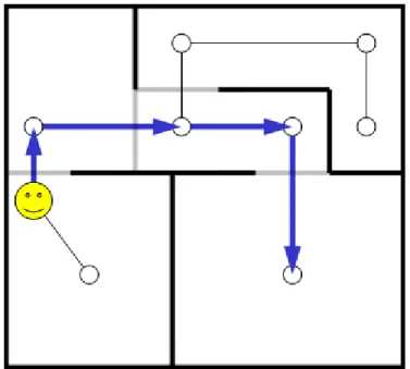
(given by the user) from another file. The nodes will move along this graph, selecting as destination a random vertex of the graph and moving there choosing the path with the minimum number of hops. It is possible to select which vertices of the graph are possible destination vertices, using the other ones just to link the paths between them. An example of the use of the CM model is shown in Figure 3.1, where black lines represent walls and grey lines represent doors.
Fig. 3.1 – Moving pattern of a node using the Constrained Mobility Model
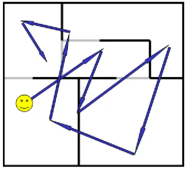
In the second sub-model, called the Shell Model, the nodes move following the rules of the Random Waypoint Model (Section 2.2.2), just avoiding crossing the external perimeter of the area and, then, completely ignoring the internal obstacles of the map, which affect just the propagation (see Fig. 3.2). In this sub-model the graph file is not read.
Fig. 3.2 – Moving pattern of a node using the Shell Model
The structure of this original model allows creating a very complex and detailed map of the obstacles, but it can barely
represent a realistic movement in an indoor environment. The nodes can or just move in a prefixed path, or move in a completely random way. It is not realistic that a node entering into a room then remains steady at one point (CM Model). On the other side, moving randomly, the internal obstacles are completely ignored and, at every step, the movement is not correlated with the previous ones (Shell Model).
In the CM Model there is also another problem. The path calculated for reaching the destination vertex is calculated minimizing the number of hops. The result can be, depending on the graph, not the shortest (usually the one most used in the real world).
3.3. IMPROVEMENTS
All the problems presented in the previous paragraph have been fixed in the new model introduced in this thesis.
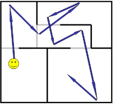
First, the Shell Model has been improved enabling the effects of the internal obstacles even for the nodes movement and not only for the signal propagation. To do this, a definition of “crossable obstacles” has been necessary. Crossable obstacles are areas of the map (e.g. doors) that do not stop the movement of the nodes, but attenuate the propagation. In Figure 3.3 the
Fig. 3.3 – Moving pattern of a node using the Modified Shell Model
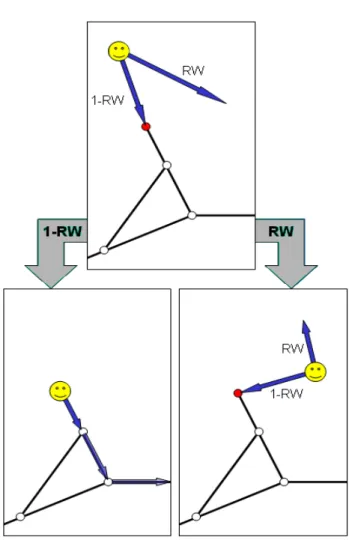
Despite this enhancement, the new model is not realistic yet. In fact, moving randomly inside an indoor scenario, the probability of leaving a room is low, so the chance of reaching rooms far from the initial one is very small. The idea is then to use both the CM and the new Shell models together, creating a new combined model. The nodes can switch from one sub-model to another, creating a more realistic moving pattern. At every step they can move in RWP model with a probability rw,
or they can jump into the graph and move to a destination vertex following the shortest pathway (calculated by the Dijkstra’s algorithm [12]) with a probability 1-rw (see Fig. 3.4).
Note that for rw=1 and rw=0 the new model returns to the original one. In practice rw is the parameter that measures the distance of the new model from the two sub-models. For a generic rw, the nodes usually move randomly in a room and use the graph to go into another room. Leaving the room is also possible during the RWP movement. In fact the node chooses a random destination in line of sight, and it can be a point belonging to another room.
Besides, it is also possible to assign different values to the parameter rw for different sub-areas of the simulation. It allows, for example, distinguishing the behaviour of the nodes in rooms (where the RWP model fits better) and in corridors (where the use of the graph is more suitable). A random speed uniformly distributed between [Vmin, Vmax] is chosen for every RWP movement and at every vertex of the path reached. It is possible to choose the use or not of the pause. With the pause, the node stops for a random time uniformly distributed between [0,T] at the end of every RWP movement and every time it reaches the destination vertex (when it uses the graph). In order to fix the problems of the original version of the model, and to provide these new features, the new model has been designed as follows. The image that contains the map of
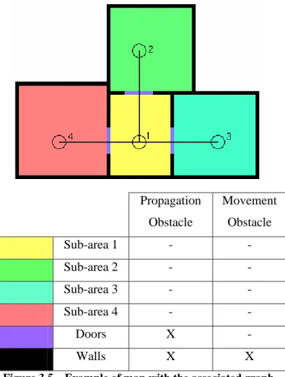
the obstacles becomes more elaborated, since every sub-area has to be painted with a different colour. In Figure 3.5 there is a simple example of a floor plan divided in sub-areas and the associated graph overlaid.
Note that the colour of the entrances is different from the one of the walls. There are two reasons: the door has different material properties from the walls. Also the door is not a real movement obstacle, it just affects the propagation. Note also that the graph must ensure that every sub-area has a destination vertex inside, in order to be used by the nodes as a reference point for jumping into the graph. When a node decides to use the graph, it first checks whether it is in line of sight with the destination vertex associated to the sub-area it is in. If it is not, the node continues moving in RWP.
The C++ Source Code of the Combined Mobility Model can be found in Appendix A.
Propagation Obstacle Movement Obstacle Sub-area 1 - - Sub-area 2 - - Sub-area 3 - - Sub-area 4 - - Doors X - Walls X X