Giovanni Fasano
A framework of conjugate
direction methods for
symmetric linear systems in
optimization
Working Paper n. 31/2013
December 2013
This Working Paper is published under the auspices of the Department of
Management at Università Ca’ Foscari Venezia. Opinions expressed herein are those
of the authors and not those of the Department or the University. The Working Paper
series is designed to divulge preliminary or incomplete work, circulated to favour
discussion and comments. Citation of this paper should consider its provisional
A Framework of Conjugate Direction Methods for
Symmetric Linear Systems in Optimization
∗Giovanni Fasano
Dept. of Management University of Venice
(December 2013)
Abstract. In this paper we introduce a parameter dependent class of Krylov-based meth-ods, namely 𝐶𝐷, for the solution of symmetric linear systems. We give evidence that in our proposal we generate sequences of conjugate directions, extending some properties of the standard Conjugate Gradient (CG) method, in order to preserve the conjugacy. For specific values of the parameters in our framework we obtain schemes equivalent to both the CG and the scaled-CG. We also prove the finite convergence of the algorithms in 𝐶𝐷, and we provide some error analysis. Finally, preconditioning is introduced for 𝐶𝐷, and we show that standard error bounds for the preconditioned CG also hold for the preconditioned 𝐶𝐷. Keywords: Krylov-based Methods, Conjugate Direction Methods, Conjugacy Loss and Error Analysis, Preconditioning.
JEL Classification Numbers: C61, C63.
MathSci Classification Numbers: 90C30, 90C06, 65K05, 49M15.
Correspondence to:
Giovanni Fasano Dept. of Management, University of Venice S.Giobbe, Cannaregio 873 30121 Venice, ITALY Phone: [++39] (041)-234-6922 Fax: [++39] (041)-234-7444 E-mail: [email protected] ∗
This author thanks the Italian national research program ‘RITMARE’, by CNR-INSEAN, National Research Council-Maritime Research Centre, for the support received.
1
Introduction
The solution of symmetric linear systems arises in a wide range of real applications [1, 2, 3], and has been carefully issued in the last 50 years, due to the increasing demand of fast and reliable solvers. Illconditioning and large number of unknowns are among the most challenging issues which may harmfully affect the solution of linear systems, in several frameworks where either structured or unstructured coefficient matrices are considered [1, 4, 5].
The latter facts have required the introduction of a considerable number of techniques, specifically aimed at tackling classes of linear systems with appointed pathologies [5, 6]. We remark that the structure of the coefficient matrix may be essential for the success of the solution methods, both in numerical analysis and optimization contexts. As an example, PDEs and PDE-constrained optimization provide two specific frameworks, where sequences of linear systems often claim for specialized and robust methods, in order to give reliable solutions.
In this paper we focus on iterative Krylov-based methods for the solution of symmetric linear systems, arising in both numerical analysis and optimization contexts. The theory detailed in the paper is not limited to consider large scale linear systems; however, since Krylov-based methods have proved their efficiency when the scale is large, without loss of generality we will implicitly assume the latter fact.
The accurate study and assessment of methods for the solution of linear systems is natu-rally expected from the community of people working on numerical analysis. That is due to their expertise and great sensibility to theoretical issues, rather than to practical algorithms implementation or software developments. This has raised a consistent literature, including manuals and textbooks, where the analysis of solution techniques for linear systems has become a keynote subject, and where essential achievements have given strong guidelines to theoreticians and practitioners from optimization [4].
We address here a parameter dependent class of CG-based methods, which can equiva-lently reduce to the CG for a suitable choice of the parameters. We firmly claim that our proposal is not primarily intended to provide an efficient alternative to the CG. On the contrary, we mainly detail a general framework of iterative methods, inspired by polarity for quadratic hypersurfaces, and based on the generation of conjugate directions. The al-gorithms in our class, thanks to the parameters in the scheme, may possibly keep under control the conjugacy loss among directions, which is often caused by finite precision in the computation. The paper is not intended to report also a significant numerical experience. Indeed, we think that there are not yet clear rules on the parameters of our proposal, for assessing efficient algorithms. Similarly, we have not currently indications that methods in our proposal can outperform the CG. On this guideline, in a separate paper we will carry on selective numerical tests, considering both symmetric linear systems from numerical analy-sis and optimization. We further prove that preconditioning can be introduced for the class of methods we propose, as a natural extension of the preconditioned CG (see also [2]).
As regards the symbols used in this paper, we indicate with 𝜆𝑚(𝐴) and 𝜆𝑀(𝐴) the
smallest/largest eigenvalue of the positive definite matrix 𝐴; moreover∥𝑣∥2
𝐴= 𝑣𝑇𝐴𝑣, where
Moore-Table 1: The CG algorithm for solving (1).
The Conjugate Gradient (CG) method Step 0: Set 𝑘 = 0, 𝑦0 ∈ ℝ, 𝑟0 := 𝑏− 𝐴𝑦0.
If 𝑟0 = 0, then STOP. Else, set 𝑝0 := 𝑟0; 𝑘 = 𝑘 + 1.
Set 𝑝−1= 0 and 𝛽−1 = 0.
Step 𝑘: Compute 𝛼𝑘−1:= 𝑟𝑘−1𝑇 𝑝𝑘−1/𝑝𝑇𝑘−1𝐴𝑝𝑘−1,
𝑦𝑘:= 𝑦𝑘−1+ 𝛼𝑘−1𝑝𝑘−1, 𝑟𝑘:= 𝑟𝑘−1− 𝛼𝑘−1𝐴𝑝𝑘−1.
If 𝑟𝑘= 0, then STOP. Else, set
– 𝛽𝑘−1 :=∥𝑟𝑘∥2/∥𝑟𝑘−1∥2, 𝑝𝑘:= 𝑟𝑘+ 𝛽𝑘−1𝑝𝑘−1
– (or equivalently set 𝑝𝑘 :=−𝛼𝑘−1𝐴𝑝𝑘−1+ (1 + 𝛽𝑘−1)𝑝𝑘−1− 𝛽𝑘−2𝑝𝑘−2)
Set 𝑘 = 𝑘 + 1, go to Step 𝑘.
Penrose pseudoinverse of matrix 𝐴. With 𝑃 𝑟𝐶(𝑣) we represent the orthogonal projection of
vector 𝑣∈ ℝ onto the convex set 𝐶 ⊆ ℝ. Finally, the symbol 𝒦𝑖(𝑏, 𝐴) indicates the Krylov
subspace span{𝑏, 𝐴𝑏, 𝐴2𝑏, . . . , 𝐴𝑖𝑏} of dimension 𝑖 + 1. All the other symbols in the paper
follow a standard notation.
Sect. 2 briefly reviews both the CG and the Lanczos process, as Krylov-subspace meth-ods, in order to highlight promising aspects to investigate in our proposal. Sect. 3 details some relevant applications of conjugate directions in optimization frameworks, motivating our interest for possible extensions of the CG. In Sects. 4 and 5 we describe our class of methods and some related properties. In Sects. 6 and 7 we show that the CG and the scaled-CG may be equivalently obtained as particular members of our class. Then, Sects. 8 and 9 contain further properties of the class of methods we propose. Finally, Sect. 10 an-alyzes the preconditioned version of our proposal, and a section of Conclusions completes the paper, including some numerical results.
2
The CG Method and the Lanczos Process
In this section we comment the method in Table 1, and we focus on the relation between the CG and the Lanczos process, as Krylov-subspace methods. In particular, the Lanczos process namely does not generate conjugate directions; however, though our proposal relies on generalizing the CG, it shares some aspects with the Lanczos iteration, too.
As we said, the CG is commonly used to iteratively solving the linear system
𝐴𝑦 = 𝑏, (1)
where 𝐴∈ ℝ𝑛×𝑛 is symmetric positive definite and 𝑏∈ ℝ𝑛. Observe that the CG is quite
often applied to a preconditioned version of the linear system (1), i.e. ℳ𝐴𝑦 = ℳ𝑏, where ℳ ≻ 0 is the preconditioner [7]. Though the theory for the CG requires 𝐴 to be positive
definite, in several practical applications it is successfully used when 𝐴 is indefinite, too [8, 9]. At Step 𝑘 the CG generates the pair of vectors 𝑟𝑘(residual) and 𝑝𝑘(search direction)
such that [2]
orthogonality property : 𝑟𝑇𝑖 𝑟𝑗 = 0, 0≤ 𝑖 ∕= 𝑗 ≤ 𝑘, (2)
conjugacy property : 𝑝𝑇𝑖 𝐴𝑝𝑗 = 0, 0≤ 𝑖 ∕= 𝑗 ≤ 𝑘. (3)
Moreover, finite convergence holds, i.e. 𝐴𝑦ℎ = 𝑏 for some ℎ ≤ 𝑛. Relations (2) yield the
Ritz-Galerkin condition 𝑟𝑘⊥ 𝒦𝑘−1(𝑟0, 𝐴), where
𝒦𝑘−1(𝑟0, 𝐴) := span{𝑏, 𝐴𝑏, 𝐴2𝑏, . . . , 𝐴𝑘−1𝑏} ≡ span{𝑟0, . . . , 𝑟𝑘−1}.
Furthermore, the direction 𝑝𝑘 is computed at Step 𝑘 imposing the conjugacy condition
𝑝𝑇𝑘𝐴𝑝𝑘−1 = 0. It can be easily proved that the latter equality implicitly satisfies relations
(3), with 𝑝0, . . . , 𝑝𝑘 linearly independent. We remark that on practical problems, due to
finite precision and roundoff in the computation of the sequences{𝑝𝑘} and {𝑟𝑘}, when ∣𝑖−𝑗∣
is large relations (2)-(3) may fail. Thus, in the practical implementation of the CG some theoretical properties may not be satisfied, and in particular when ∣𝑖 − 𝑗∣ increases the conjugacy properties (3) may progressively be lost. As detailed in [10, 11, 12, 13] the latter fact may have dramatic consequences also in optimization frameworks (see also Sect. 3 for details). To our purposes we note that in Table 1, at Step 𝑘 of the CG, the direction 𝑝𝑘 is
usually computed as
𝑝𝑘 := 𝑟𝑘+ 𝛽𝑘−1𝑝𝑘−1, (4)
but an equivalent expression is (see also Theorem 5.4 in [14])
𝑝𝑘:=−𝛼𝑘−1𝐴𝑝𝑘−1+ (1 + 𝛽𝑘−1)𝑝𝑘−1− 𝛽𝑘−2𝑝𝑘−2, (5)
which we would like to generalize in our proposal. Note also that in exact arithmetics the property (3) is iteratively fulfilled by both (4) and (5).
The Lanczos process (and its preconditioned version) is another Krylov-based method, widely used to tridiagonalize the matrix 𝐴 in (1). Unlike the CG method, here the matrix 𝐴 may be possibly indefinite, and the overall method is slightly more expensive than the CG, since further computation is necessary to solve the resulting tridiagonal system. Similarly to the CG, the Lanczos process generates at Step 𝑘 the sequence {𝑢𝑘} (Lanczos vectors)
which satisfies
orthogonality property : 𝑢𝑇𝑖 𝑢𝑗 = 0, 0≤ 𝑖 ∕= 𝑗 ≤ 𝑘,
and yields finite convergence in at most 𝑛 steps. However, unlike the CG the Lanczos process is not explicitly inspired by polarity, in order to generate the orthogonal vectors. We recall that the CG and the Lanczos process are 3-term recurrence methods, in other words, for 𝑘≥ 1
𝑝𝑘+1∈ span{𝐴𝑝𝑘, 𝑝𝑘, 𝑝𝑘−1}, for the CG
When 𝐴 is positive definite, a full theoretical correspondence between the sequence{𝑟𝑘} of
the CG and the sequence{𝑢𝑘} of the Lanczos process may be fruitfully used in optimization
problems (see also [10, 15, 16]), being 𝑢𝑘 = 𝑠𝑘
𝑟𝑘
∥𝑟𝑘∥
, 𝑠𝑘∈ {−1, +1}.
The class 𝐶𝐷 proposed in this paper provides a framework, which encompasses the CG and to some extent resembles the Lanczos iteration, since a 3-term recurrence is exploited. In particular, the 𝐶𝐷 generates both conjugate directions (as the CG) and orthogonal residuals (as the CG and the Lanczos process). Moreover, similarly to the CG, the 𝐶𝐷 yields a 3-term recurrence with respect to conjugate directions. As we remarked, our proposal draws its inspiration from the idea of possibly attenuating the conjugacy loss of the CG, which may occur in (3) when ∣𝑖 − 𝑗∣ is large.
3
Conjugate Directions for Optimization Frameworks
Optimization frameworks offer plenty of symmetric linear systems where CG-based meth-ods are often specifically preferable with respect to other solvers. Here we justify this statement by briefly describing the potential use of conjugate directions within truncated Newton schemes. The latter methods strongly prove their efficiency when applied to large scale problems, where they rely on the proper computation of search directions, as well as truncation rules (see [17]).
As regards the computation of search directions, suppose at the outer iteration ℎ of the truncated scheme we perform 𝑚 steps of the CG, in order to compute the approximate solution 𝑑𝑚
ℎ to the linear system (Newton’s equation)
∇2𝑓 (𝑧ℎ)𝑑 =−∇𝑓(𝑧ℎ).
When 𝑧ℎ is close enough to the solution 𝑧∗ (minimum point) then possibly ∇2𝑓 (𝑧ℎ) ≻ 0.
Thus, the conjugate directions 𝑝1, . . . , 𝑝𝑚 and the coefficients 𝛼1, . . . , 𝛼𝑚 are generated as
in Table 1, so that the following vectors can be formed 𝑑𝑚ℎ = 𝑚 ∑ 𝑖=1 𝛼𝑖𝑝𝑖, 𝑑𝑃ℎ = ∑ 𝑖∈𝐼𝑃 ℎ 𝛼𝑖𝑝𝑖, 𝐼ℎ𝑃 ={𝑖 ∈ {1, . . . , 𝑚} : 𝑝𝑇𝑖 ∇2𝑓 (𝑧ℎ)𝑝𝑖 > 0} , 𝑑𝑁ℎ = ∑ 𝑖∈𝐼𝑁 ℎ 𝛼𝑖𝑝𝑖, 𝐼ℎ𝑁 ={𝑖 ∈ {1, . . . , 𝑚} : 𝑝𝑇𝑖 ∇2𝑓 (𝑧ℎ)𝑝𝑖< 0} , 𝑠ℎ = 𝑝ℓ ∥𝑟ℓ∥ , ℓ = arg min𝑖∈{1,...,𝑚}{ 𝑝 𝑇 𝑖 ∇2𝑓 (𝑧ℎ)𝑝𝑖 ∥𝑟𝑖∥2 : 𝑝𝑇𝑖 ∇2𝑓 (𝑧ℎ)𝑝𝑖< 0 } . (6)
Observe that 𝑑𝑚ℎ approximates in some sense Newton’s direction at the outer iteration ℎ, and as described in [11, 12, 18, 19] the vectors 𝑑𝑚
ℎ, 𝑑𝑃ℎ and 𝑑𝑁ℎ can be used/combined to
provide fruitful search directions to the optimization framework. Moreover, 𝑑𝑁
suitably used/combined to compute a so called negative curvature direction ‘𝑠𝑚
ℎ’, which can
possibly force second order convergence for the overall truncated optimization scheme (see [18] for details). The conjugacy property is essential for computing the vectors (6). i.e. to design efficient truncated Newton methods. Thus, introducing CG-based schemes which deflate conjugacy loss might be of great importance.
On the other hand, at the outer iteration ℎ effective truncation rules typically attempt to assess the parameter 𝑚 in (6), as described in [17, 20, 21]. I.e., they monitor the decrease of the quadratic local model
𝑄ℎ(𝑑𝑚ℎ) := 𝑓 (𝑧ℎ) +∇𝑓(𝑧ℎ)𝑇(𝑑𝑚ℎ) +
1 2(𝑑
𝑚
ℎ)𝑇∇2𝑓 (𝑧ℎ)(𝑑𝑚ℎ)
when∇2𝑓 (𝑧ℎ)≻ 0, so that the parameter 𝑚 is chosen to satisfy some conditions, including
𝑄ℎ(𝑑𝑚ℎ)− 𝑄ℎ(𝑑𝑚−1ℎ )
𝑄ℎ(𝑑𝑚ℎ)/𝑚 ≤ 𝛼,
for some 𝛼∈ ]0, 1[.
Thus, again the correctness of conjugacy properties among the directions 𝑝1, . . . , 𝑝𝑚,
gen-erated while solving Newton’s equation, may be essential both for an accurate solution of Newton’s equation (which is a linear system) and to the overall efficiency of the truncated optimization method.
4
Our Proposal: the 𝐶𝐷 Class
Before introducing our proposal for a new general framework of CG-based algorithms, we consider here some additional motivations for using the CG. The careful use of the latter theory is in our opinion a launching pad for possible extensions of the CG. On this guideline, recalling the contents in Sect. 3, now we summarize some critical aspects of the CG:
1. the CG works iteratively and at any iteration the overall computational effort is only 𝑂(𝑛2) (since the CG is a Krylov-subspace method);
2. the conjugate directions generated by the CG are linearly independent, so that at most 𝑛 iterations are necessary to address the solution;
3. the current conjugate direction 𝑝𝑘+1 is computed by simply imposing the conjugacy
with respect to the direction 𝑝𝑘 (computed) in the previous iteration. This
automat-ically yields that 𝑝𝑇
𝑘+1𝐴𝑝𝑖 = 0, for any 𝑖≤ 𝑘, too.
As a matter of fact, for the design of possible general frameworks including CG-based methods, the items 1. and 2. are essential in order to respectively control the computational effort and ensure the finite convergence.
On the other hand, altering the item 3. might be harmless for the overall iterative process, and might possibly yield some fruitful generalizations. That is indeed the case of our proposal, where the item 3. is modified with respect to the CG. The latter modification depends on a parameter which is user/problem-dependent, and may be set in order to
Table 2: The parameter dependent class 𝐶𝐷 of CG-based algorithms for solving (1).
The 𝐶𝐷 class
Step 0: Set 𝑘 = 0, 𝑦0 ∈ ℝ𝑛, 𝑟0 := 𝑏− 𝐴𝑦0, 𝛾0 ∈ ℝ ∖ {0}.
If 𝑟0= 0, then STOP. Else, set 𝑝0:= 𝑟0, 𝑘 = 𝑘 + 1.
Compute 𝑎0 := 𝑟0𝑇𝑝0/𝑝𝑇0𝐴𝑝0,
𝑦1 := 𝑦0+ 𝑎0𝑝0, 𝑟1:= 𝑟0− 𝑎0𝐴𝑝0.
If 𝑟1= 0, then STOP. Else, set 𝜎0:= 𝛾0∥𝐴𝑝0∥2/𝑝𝑇0𝐴𝑝0,
𝑝1 := 𝛾0𝐴𝑝0− 𝜎0𝑝0, 𝑘 = 𝑘 + 1.
Step 𝑘: Compute 𝑎𝑘−1:= 𝑟𝑘−1𝑇 𝑝𝑘−1/𝑝𝑇𝑘−1𝐴𝑝𝑘−1,
𝑦𝑘:= 𝑦𝑘−1+ 𝑎𝑘−1𝑝𝑘−1, 𝑟𝑘:= 𝑟𝑘−1− 𝑎𝑘−1𝐴𝑝𝑘−1.
If 𝑟𝑘= 0, then STOP. Else, set 𝜎𝑘−1 := 𝛾𝑘−1 ∥𝐴𝑝𝑘−1∥
2 𝑝𝑇 𝑘−1𝐴𝑝𝑘−1, 𝜔𝑘−1 := 𝛾𝑘−1(𝐴𝑝𝑘−1) 𝑇𝐴𝑝 𝑘−2 𝑝𝑇 𝑘−2𝐴𝑝𝑘−2 = 𝛾𝑘−1 𝛾𝑘−2 𝑝𝑇 𝑘−1𝐴𝑝𝑘−1 𝑝𝑇 𝑘−2𝐴𝑝𝑘−2, 𝛾𝑘−1∈ ℝ ∖ {0} 𝑝𝑘:= 𝛾𝑘−1𝐴𝑝𝑘−1− 𝜎𝑘−1𝑝𝑘−1− 𝜔𝑘−1𝑝𝑘−2, 𝑘 = 𝑘 + 1. Go to Step 𝑘.
further compensate or correct the conjugacy loss among directions, due to roundoff and finite precision.
We sketch in Table 2 our new CG-based class of algorithms, namely 𝐶𝐷. The compu-tation of the direction 𝑝𝑘 at Step 𝑘 reveals the main difference between the CG and 𝐶𝐷. In
particular, in Table 2 the pair of coefficients 𝜎𝑘−1 and 𝜔𝑘−1 is computed so that explicitly1
𝑝𝑇
𝑘𝐴𝑝𝑘−1 = 0
𝑝𝑇
𝑘𝐴𝑝𝑘−2 = 0,
(8)
i.e. in Cartesian coordinates the conjugacy between the direction 𝑝𝑘and both the directions
𝑝𝑘−1 and 𝑝𝑘−2 is directly imposed, as specified by (3). As detailed in Sect. 2, imposing the
double condition (8) allows to possibly recover the conjugacy loss in the sequence{𝑝𝑖}.
On the other hand, the residual 𝑟𝑘 at Step 𝑘 of Table 2 is computed by imposing
the orthogonality condition 𝑟𝑘𝑇𝑝𝑘−1 = 0, as in the standard CG. The resulting method is
evidently a bit more expensive than the CG, requiring one additional inner product per step, as long as an additional scalar to compute and an additional 𝑛-vector to store. From Table
1
A further generalization might be obtained computing 𝜎𝑘−1 and 𝜔𝑘−1 so that
⎧ ⎨ ⎩ 𝑝𝑇𝑘𝐴(𝛾𝑘−1𝐴𝑝𝑘−1− 𝜎𝑘−1𝑝𝑘−1) = 0 𝑝𝑇 𝑘𝐴𝑝𝑘−2 = 0. (7)
2 it is also evident that 𝐶𝐷 provides a 3-term recurrence with respect to the conjugate directions.
In addition, observe that the residual 𝑟𝑘 is computed at Step 𝑘 of 𝐶𝐷 only to check for
the stopping condition, and is not directly involved in the computation of 𝑝𝑘. Hereafter in
this section we briefly summarize the basic properties of the class 𝐶𝐷.
Assumption 4.1 The matrix 𝐴 in (1) is symmetric positive definite. Moreover, the se-quence {𝛾𝑘} in Table 2 is such that 𝛾𝑘∕= 0, for any 𝑘 ≥ 0.
Note that as for the CG, the Assumption 4.1 is required for theoretical reasons. However, the 𝐶𝐷 class may in principle be used also in several cases when 𝐴 is indefinite, provided that 𝑝𝑇
𝑘𝐴𝑝𝑘∕= 0, for any 𝑘 ≥ 0.
Lemma 4.1 Let Assumption 4.1 hold. At Step 𝑘 of the 𝐶𝐷 class, with 𝑘≥ 0, we have 𝐴𝑝𝑗 ∈ span{𝑝𝑗+1, 𝑝𝑗, 𝑝max{0,𝑗−1}} , 𝑗 ≤ 𝑘. (9)
Proof
From the Step 0 relation (9) holds for 𝑗 = 0. Then, for 𝑗 = 1, . . . , 𝑘− 1 the Step 𝑗 + 1 of
𝐶𝐷 directly yields (9). □
Theorem 4.2 [Conjugacy] Let Assumption 4.1 hold. At Step 𝑘 of the 𝐶𝐷 class, with 𝑘 ≥ 0, the directions 𝑝0, 𝑝1, . . . , 𝑝𝑘 are mutually conjugate, i.e. 𝑝𝑇𝑖 𝐴𝑝𝑗 = 0, with 0≤ 𝑖 ∕=
𝑗≤ 𝑘. Proof
The statement holds for Step 0, as a consequence of the choice of the coefficient 𝜎0. Suppose
it holds for 𝑘− 1; then, we have for 𝑗 ≤ 𝑘 − 1
𝑝𝑇𝑘𝐴𝑝𝑗 = (𝛾𝑘−1𝐴𝑝𝑘−1− 𝜎𝑘−1𝑝𝑘−1− 𝜔𝑘−1𝑝𝑘−2)𝑇 𝐴𝑝𝑗
= (𝛾𝑘−1𝐴𝑝𝑘−1)𝑇𝐴𝑝𝑗− 𝜎𝑘−1𝑝𝑇𝑘−1𝐴𝑝𝑗− 𝜔𝑘−1𝑝𝑇𝑘−2𝐴𝑝𝑗 = 0.
In particular, for 𝑗 = 𝑘− 1 and 𝑗 = 𝑘 − 2 the choice of the coefficients 𝜎𝑘−1 and 𝜔𝑘−1,
and the inductive hypothesis, yield directly 𝑝𝑇
𝑘𝐴𝑝𝑘−1 = 𝑝𝑇𝑘𝐴𝑝𝑘−2 = 0. For 𝑗 < 𝑘− 2, the
inductive hypothesis and Lemma 4.1 again yield the conjugacy property. □ Lemma 4.3 Let Assumption 4.1 hold. Given the 𝐶𝐷 class, we have for 𝑘≥ 2
(𝐴𝑝𝑘)𝑇(𝐴𝑝𝑖) = ⎧ ⎨ ⎩ ∥𝐴𝑝𝑘∥2, if 𝑖 = 𝑘, 1 𝛾𝑘−1𝑝 𝑇 𝑘𝐴𝑝𝑘, if 𝑖 = 𝑘− 1, ∅, if 𝑖≤ 𝑘 − 2. Proof
The statement is a trivial consequence of Step 𝑘 of the 𝐶𝐷, Lemma 4.1 and Theorem 4.2. □
Observe that from the previous lemma, a simplified expression for the coefficient 𝜔𝑘−1,
at Step 𝑘 of 𝐶𝐷 is available, inasmuch as 𝜔𝑘−1 = 𝛾𝑘−1 𝛾𝑘−2 ⋅ 𝑝𝑇 𝑘−1𝐴𝑝𝑘−1 𝑝𝑇 𝑘−2𝐴𝑝𝑘−2 . (10)
Relation (10) has a remarkable importance: it avoids the storage of the vector 𝐴𝑝𝑘−2 at
Step 𝑘, requiring only the storage of the quantity 𝑝𝑇𝑘−2𝐴𝑝𝑘−2. Also observe that unlike the
CG, the sequence {𝑝𝑘} in 𝐶𝐷 is computed independently of the sequence {𝑟𝑘}. Moreover,
as we said the residual 𝑟𝑘 is simply computed at Step 𝑘 in order to check the stopping
condition for the algorithm.
The following result proves that the 𝐶𝐷 class recovers the main theoretical properties of the standard CG.
Theorem 4.4 [Orthogonality] Let Assumption 4.1 hold. Let 𝑟𝑘+1∕= 0 at Step 𝑘+1 of the
𝐶𝐷 class, with 𝑘≥ 0. Then, the directions 𝑝0, 𝑝1, . . . , 𝑝𝑘 and the residuals 𝑟0, 𝑟1, . . . , 𝑟𝑘+1
satisfy
𝑟𝑇𝑘+1𝑝𝑗 = 0, 𝑗≤ 𝑘, (11)
𝑟𝑇𝑘+1𝑟𝑗 = 0, 𝑗≤ 𝑘. (12)
Proof
From Step 𝑘 + 1 of 𝐶𝐷 we have 𝑟𝑘+1= 𝑟𝑘− 𝑎𝑘𝐴𝑝𝑘= 𝑟𝑗−∑𝑘𝑖=𝑗𝑎𝑖𝐴𝑝𝑖, for any 𝑗≤ 𝑘. Then,
from Theorem 4.2 and the choice of coefficient 𝛼𝑗 we obtain
𝑟𝑘+1𝑇 𝑝𝑗 = ⎛ ⎝𝑟𝑗− 𝑘 ∑ 𝑖=𝑗 𝑎𝑖𝐴𝑝𝑖 ⎞ ⎠ 𝑇 𝑝𝑗 = 𝑟𝑗𝑇𝑝𝑗− 𝑘 ∑ 𝑖=𝑗 𝑎𝑖𝑝𝑇𝑖 𝐴𝑝𝑗 = 0, 𝑗≤ 𝑘,
which proves (11). As regards relation (12), for 𝑘 = 0 we obtain from the choice of 𝑎0
𝑟𝑇
1𝑟0 = 𝑟1𝑇𝑝0 = 0.
Then, assuming by induction that (12) holds for 𝑘− 1, we have 𝑟𝑇𝑘+1𝑟𝑗 = (𝑟𝑘− 𝑎𝑘𝐴𝑝𝑘)𝑇 𝑟𝑗 = (𝑟𝑘− 𝑎𝑘𝐴𝑝𝑘)𝑇 ( 𝑟0− 𝑗−1 ∑ 𝑖=0 𝑎𝑖𝐴𝑝𝑖 ) = 𝑟𝑇𝑘𝑟0− 𝑗−1 ∑ 𝑖=0 𝑎𝑖𝑟𝑇𝑘𝐴𝑝𝑖− 𝑎𝑘𝑝𝑇𝑘𝐴𝑟0+ 𝑗−1 ∑ 𝑖=0 𝑎𝑖𝑎𝑘(𝐴𝑝𝑘)𝑇𝐴𝑝𝑖, 𝑗≤ 𝑘.
The inductive hypothesis and Theorem 4.2 yield for 𝑗≤ 𝑘 (in the next relation when 𝑖 = 0 then 𝑝𝑖−1≡ 0) 𝑟𝑘+1𝑇 𝑟𝑗 = − 𝑗−1 ∑ 𝑖=0 𝑎𝑖𝑟𝑇𝑘 𝛾𝑖 (𝑝𝑖+1+ 𝜎𝑖𝑝𝑖+ 𝜔𝑖𝑝𝑖−1) + 𝑗−1 ∑ 𝑖=0 𝑎𝑖𝑎𝑘(𝐴𝑝𝑘)𝑇𝐴𝑝𝑖. (13)
Therefore, if 𝑗 = 𝑘 the relation (11) along with Lemma 4.3 and the choice of 𝑎𝑘 yield 𝑟𝑘+1𝑇 𝑟𝑘 = − 𝑎𝑘−1 𝛾𝑘−1 𝑟𝑘𝑇𝑝𝑘+ 𝑎𝑘−1𝑎𝑘 𝛾𝑘−1 𝑝𝑇𝑘𝐴𝑝𝑘 = 0.
On the other hand, if 𝑗 < 𝑘 in (13), the inductive hypothesis, relation (11) and Lemma 4.3
yield (12). □
Finally, we prove that likewise the CG, in at most 𝑛 iterations 𝐶𝐷 determines the solution of the linear system (1), so that finite convergence holds.
Lemma 4.5 [Finite convergence] Let Assumption 4.1 hold. At Step 𝑘 of the 𝐶𝐷 class, with 𝑘≥ 0, the vectors 𝑝0, . . . , 𝑝𝑘are linearly independent. Moreover, in at most 𝑛 iterations
the 𝐶𝐷 class computes the solution of the linear system (1), i.e. 𝐴𝑦ℎ = 𝑏, for some ℎ≤ 𝑛.
Proof
The proof follows very standard guidelines (the reader may also refer to [22]). Thus, by (11) an integer 𝑚≤ 𝑛 exists such that 𝑟𝑚 = 𝑏− 𝐴𝑦𝑚= 0. Then, if 𝑦∗ is the solution of (1),
we have 0 = 𝑏− 𝐴𝑦𝑚= 𝐴𝑦∗− 𝐴 [ 𝑦0+ 𝑚−1 ∑ 𝑖=0 𝑎𝑖𝑝𝑖 ] ⇐⇒ 𝑦∗ = 𝑦0+ 𝑚−1 ∑ 𝑖=0 𝑎𝑖𝑝𝑖. □ Remark 1 Observe that there is the additional chance to replace the Step 0 in Table 2, with the following CG-like Step 0𝑏
Step 0𝑏: Set 𝑘 = 0, 𝑦0∈ ℝ𝑛, 𝑟0 := 𝑏− 𝐴𝑦0.
If 𝑟0 = 0, then STOP. Else, set 𝑝0 := 𝑟0, 𝑘 = 𝑘 + 1.
Compute 𝑎0 := 𝑟0𝑇𝑝0/𝑝𝑇0𝐴𝑝0,
𝑦1:= 𝑦0+ 𝑎0𝑝0, 𝑟1 := 𝑟0− 𝑎0𝐴𝑝0.
If 𝑟1 = 0, then STOP. Else, set 𝜎0 :=−∥𝑟1∥2/∥𝑟0∥2,
𝑝1 := 𝑟1+ 𝜎0𝑝0, 𝑘 = 𝑘 + 1.
5
Further Properties for 𝐶𝐷
In this section we consider some properties of 𝐶𝐷 which represent a natural extension of analogous properties of the CG. To this purpose we introduce the error function
𝑓 (𝑦) := 1 2(𝑦− 𝑦
∗)𝑇𝐴(𝑦
− 𝑦∗), with 𝐴𝑦∗= 𝑏, (14)
and the quadratic functional 𝑔(𝑦) := 1
2(𝑦− 𝑦𝑖)
𝑇𝐴(𝑦
− 𝑦𝑖), with 𝑖∈ {1, . . . , 𝑚}, (15)
which satisfy 𝑓 (𝑦) ≥ 0, 𝑔(𝑦) ≥ 0, for any 𝑦 ∈ ℝ𝑛, when 𝐴 ર 0. Then, we have the
following result, where we prove minimization properties of the error function 𝑓 (𝑦) (see also Theorem 6.1 in [14]) and 𝑔(𝑦) (see also [23]), along with the fact that 𝐶𝐷 provides a suitable approximation of the inverse matrix 𝐴−1, too.
Theorem 5.1 [Further Properties] Consider the linear system (1) with 𝐴ર 0, and the functions 𝑓 (𝑦) and 𝑔(𝑦) in (14)-(15). Assume that the 𝐶𝐷 has performed 𝑚 + 1 iterations, with 𝑚 + 1≤ 𝑛 and 𝐴𝑦𝑚+1= 𝑏. Let 𝛾𝑖−1 ∕= 0 with 𝑖 ≥ 1. Then,
∙ 𝜎0 minimizes 𝑔(𝑦) on the manifold (𝑦1+ 𝛾0𝐴𝑝0) + span{𝑝0},
∙ 𝜎𝑖−1 and 𝜔𝑖−1, 𝑖 = 2, . . . , 𝑚, minimize 𝑔(𝑦) on the two dimensional manifold (𝑦𝑖+
𝛾𝑖−1𝐴𝑝𝑖−1) + span{𝑝𝑖−1, 𝑝𝑖−2}. Moreover, 𝑓 (𝑦𝑖+ 𝑎𝑖𝑝𝑖) = 𝑓 (𝑦𝑖)− ( 𝛾𝑖−1 𝑎𝑖−1 )2 ∥𝑟𝑖∥4 𝑝𝑇 𝑖 𝐴𝑝𝑖 , 𝑖 = 1, . . . , 𝑚, (16) and we have [ 𝐴+− 𝑚 ∑ 𝑖=0 𝑝𝑖𝑝𝑇𝑖 𝑝𝑇 𝑖 𝐴𝑝𝑖 ] 𝑟0= 0, for any 𝑦0∈ ℝ𝑛. (17) Proof
Observe that for 𝑖 = 1, indicating in Table 2 𝑝1= 𝛾0𝐴𝑝0+ 𝑎𝑝0, with 𝑎∈ ℝ, by (15)
𝑔(𝑦2) = 𝑔(𝑦1+ 𝑎1𝑝1) =𝑎 2 1 2 (𝛾0𝐴𝑝0+ 𝑎𝑝0) 𝑇𝐴(𝛾 0𝐴𝑝0+ 𝑎𝑝0) and we have 0 = ∂𝑔(𝑦2) ∂𝑎 𝑎=𝑎∗ = 𝑎21𝑝𝑇0𝐴(𝛾0𝐴𝑝0+ 𝑎∗𝑝0) ⇐⇒ 𝑎∗ =−𝛾0∥𝐴𝑝0∥ 2 𝑝𝑇 0𝑎𝑝0 =−𝜎0.
For 𝑖≥ 2, if we indicate in Table 2 𝑝𝑖 = 𝛾𝑖−1𝐴𝑝𝑖−1+ 𝑏𝑝𝑖−1+ 𝑐𝑝𝑖−2, with 𝑏, 𝑐∈ ℝ, then by
(15) 𝑔(𝑦𝑖+ 𝑎𝑖𝑝𝑖) = 𝑎 2 𝑖 2 (𝛾𝑖−1𝐴𝑝𝑖−1+ 𝑏𝑝𝑖−1+ 𝑐𝑝𝑖−2) 𝑇𝐴(𝛾 𝑖−1𝐴𝑝𝑖−1+ 𝑏𝑝𝑖−1+ 𝑐𝑝𝑖−2)
and by Assumption 4.1, after some computation, the equalities ⎧ ⎨ ⎩ ∂𝑔(𝑦𝑖+1) ∂𝑏 𝑏=𝑏∗, 𝑐=𝑐∗ = ∂𝑔(𝑦𝑖+ 𝑎𝑖𝑝𝑖) ∂𝑏 𝑏=𝑏∗, 𝑐=𝑐∗ = 0 ∂𝑔(𝑦𝑖+1) ∂𝑐 𝑏=𝑏∗, 𝑐=𝑐∗ = ∂𝑔(𝑦𝑖+ 𝑎𝑖𝑝𝑖) ∂𝑐 𝑏=𝑏∗, 𝑐=𝑐∗ = 0 imply the unique solution
⎧ ⎨ ⎩ 𝑏∗ =−𝛾𝑖−1 ∥𝐴𝑝𝑖−1∥ 2 𝑝𝑇 𝑖−1𝐴𝑝𝑖−1 =−𝜎𝑖−1 𝑐∗ =−𝛾𝑖−1 (𝐴𝑝𝑖−1)𝑇(𝐴𝑝𝑖−2) 𝑝𝑇 𝑖−2𝐴𝑝𝑖−2 =−𝛾𝑖−1 𝛾𝑖−2 𝑝𝑇 𝑖−1𝐴𝑝𝑖−1 𝑝𝑇 𝑖−2𝐴𝑝𝑖−2 =−𝜔𝑖−1. (18)
As regards (16), from Table 2 we have that for any 𝑖≥ 1 𝑓 (𝑦𝑖+ 𝑎𝑖𝑝𝑖) = 𝑓 (𝑦𝑖) + 𝑎𝑖(𝑦𝑖− 𝑦∗)𝑇𝐴𝑝𝑖+ 1 2𝑎 2 𝑖𝑝𝑇𝑖 𝐴𝑝𝑖 = 𝑓 (𝑦𝑖)− 𝑎𝑖𝑟𝑖𝑇𝑝𝑖+ 1 2𝑎 2 𝑖𝑝𝑇𝑖 𝐴𝑝𝑖 = 𝑓 (𝑦𝑖)− 1 2 (𝑟𝑇 𝑖 𝑝𝑖)2 𝑝𝑇 𝑖𝐴𝑝𝑖 . (19)
Now, since 𝑟𝑖 = 𝑟𝑖−1− 𝑎𝑖−1𝐴𝑝𝑖−1 we have
𝑝𝑖 = 𝛾𝑖−1 ( 𝑟𝑖−1− 𝑟𝑖 𝑎𝑖−1 ) − 𝜎𝑖−1𝑝𝑖−1, 𝑖 = 1, 𝑝𝑖 = 𝛾𝑖−1 ( 𝑟𝑖−1− 𝑟𝑖 𝑎𝑖−1 ) − 𝜎𝑖−1𝑝𝑖−1− 𝜔𝑖−1𝑝𝑖−2, 𝑖≥ 2,
so that from Theorem 4.4
𝑟𝑖𝑇𝑝𝑖 =−
𝛾𝑖−1
𝑎𝑖−1∥𝑟𝑖∥ 2.
The latter relation and (19) yield (16).
As regards (17), since 𝐴𝑦𝑚+1= 𝑏 then 𝑏∈ 𝑅(𝐴), and from Table 2 then 𝑟𝑖∈ 𝒦𝑖(𝑏, 𝐴)⊆
𝑅(𝐴), 𝑖 = 0, . . . , 𝑚, where 𝒦𝑖+1(𝑏, 𝐴) ⊇ 𝒦𝑖(𝑏, 𝐴). In addition, by the definition of
Moore-Penrose pseudoinverse matrix (see [24]), and since 𝑦𝑚+1 is a solution of (1) we have
𝑃 𝑟𝑅(𝐴)(𝑦𝑚+1) = 𝐴+𝑏 = 𝐴+(𝑟0+ 𝐴𝑦0)
= 𝐴+𝑟0+ 𝑃 𝑟𝑅(𝐴)(𝑦0). (20)
Moreover, 𝑦𝑚+1= 𝑦0+∑𝑚𝑖=0𝑎𝑖𝑝𝑖 and by induction 𝑝𝑖∈ 𝒦𝑖(𝑏, 𝐴)⊆ 𝑅(𝐴), thus
𝑃 𝑟𝑅(𝐴)(𝑦𝑚+1) = 𝑃 𝑟𝑅(𝐴)(𝑦0) + 𝑃 𝑟𝑅(𝐴) ( 𝑚 ∑ 𝑖=0 𝑎𝑖𝑝𝑖 ) = 𝑃 𝑟𝑅(𝐴)(𝑦0) + 𝑚 ∑ 𝑖=0 𝑎𝑖𝑝𝑖. (21)
By (20), (21) and recalling that for 𝐶𝐷 we have 𝑝𝑇
𝑖 𝑟𝑖 = 𝑝𝑇𝑖(𝑟𝑖−1− 𝑎𝑖−1𝐴𝑝𝑖−1) = 𝑝𝑇𝑖 𝑟𝑖−1 = ⋅ ⋅ ⋅ = 𝑝𝑇 𝑖 𝑟0, we obtain 𝐴+𝑟0 = 𝑚 ∑ 𝑖=0 𝑎𝑖𝑝𝑖 = 𝑚 ∑ 𝑖=0 𝑝𝑇 𝑖 𝑟𝑖 𝑝𝑇 𝑖 𝐴𝑝𝑖 𝑝𝑖 = 𝑚 ∑ 𝑖=0 𝑝𝑖𝑝𝑇𝑖 𝑝𝑇 𝑖 𝐴𝑝𝑖 𝑟0, which yields (17). □
Observe that the result in (18) may be seen as a consequence of the Theorem 3.6 in [8], which holds for a general quadratic functional 𝑔(𝑥).
Theorem 5.1 [Inverse Approximation] Let Assumption 4.1 hold and suppose that 𝐴𝑦𝑚+1 = 𝑏, where 𝑦𝑚+1 is computed by 𝐶𝐷 and 𝑚 = 𝑛− 1. Then, we have
𝐴−1 = 𝑛−1 ∑ 𝑖=0 𝑝𝑖𝑝𝑇𝑖 𝑝𝑇 𝑖 𝐴𝑝𝑖 . Proof
The proof follows from (17), recalling that the directions 𝑝0, . . . , 𝑝𝑛−1 are linearly
indepen-dent and when 𝐴 is nonsingular 𝐴−1≡ 𝐴+. □
6
Basic Relation Between the CG and 𝐶𝐷
Observe that the geometry of vectors{𝑝𝑘} and {𝑟𝑘} in 𝐶𝐷 might be substantially different
with respect to the CG. Indeed, in the latter scheme the relation 𝑝𝑘 = 𝑟𝑘 + 𝛽𝑘−1𝑝𝑘−1
implies 𝑟𝑇
𝑘𝑝𝑘 = ∥𝑟𝑘∥2 > 0, for any 𝑘. On the contrary, for the 𝐶𝐷, using relation 𝑟𝑘 =
𝑟𝑘−1− 𝑎𝑘−1𝐴𝑝𝑘−1 and Theorem 4.4 we have that possibly 𝑟𝑘𝑇𝑝𝑘∕= ∥𝑟𝑘∥2 and
𝑝𝑇 𝑘𝐴𝑝𝑘 𝑝𝑇 𝑘−1𝐴𝑝𝑘−1 = 𝛾𝑘−1 (𝐴𝑝𝑘−1)𝑇𝐴𝑝𝑘 𝑝𝑇 𝑘−1𝐴𝑝𝑘−1 = − 𝛾𝑘−1∥𝑟𝑘∥ 2 𝑎𝑘𝑎𝑘−1𝑝𝑇𝑘−1𝐴𝑝𝑘−1 = −𝛾𝑘−1 ∥𝑟𝑘∥ 2𝑝𝑇 𝑘𝐴𝑝𝑘 (𝑟𝑇 𝑘𝑝𝑘)(𝑟𝑘−1𝑇 𝑝𝑘−1) , so that when 𝐴≻ 0 we obtain
𝛾𝑘−1(𝑟𝑘𝑇𝑝𝑘)(𝑟𝑘−1𝑇 𝑝𝑘−1) < 0. (22)
The latter result is a consequence of the fact that in the 𝐶𝐷 class, the direction 𝑝𝑘 is not
generated directly using the vector 𝑟𝑘. In addition, a similar conclusion also holds if we
compute the quantity 𝑝𝑇
𝑘𝑝𝑗 > 0, 𝑘∕= 𝑗, for both the CG and the 𝐶𝐷 (see also Theorem 5.3
in [14]).
As another difference between the CG and 𝐶𝐷, we have that in the first algorithm the coefficient 𝛽𝑘−1, at Step 𝑘 in Table 1, is always positive. On the other hand, the coefficients
𝛾𝑘−1, 𝜎𝑘−1 and 𝜔𝑘−1 at Step 𝑘 of Table 2 might be possibly negative.
We also observe that the CG in Table 1 simply stores at Step 𝑘 the vectors 𝑟𝑘−1 and
𝑝𝑘−1, in order to compute respectively 𝑟𝑘 and 𝑝𝑘. On the other hand, at Step 𝑘 the 𝐶𝐷
requires the storage of one additional vector, which contains some information from iteration 𝑘− 2. The idea of storing at Step 𝑘 some information from iterations preceding Step 𝑘 − 1 is not new for Krylov-based methods. Some examples, which differ from our approach, may be found in [7], for unsymmetric linear systems.
In any case, it is not difficult to verify that the CG may be equivalently obtained from 𝐶𝐷, setting 𝛾𝑘−1=−𝛼𝑘−1, for 𝑘 = 1, 2, . . ., in Table 2. Indeed, though in Table 1 the
coeffi-cient 𝛽𝑘−1 explicitly imposes the conjugacy only between 𝑝𝑘 and 𝑝𝑘−1, the pair (𝛼𝑘−1, 𝛽𝑘−1)
Step 𝑘 of Table 2, we want to show that setting 𝛾𝑘−1=−𝛼𝑘−1 in Table 2 we obtain ⎧ ⎨ ⎩ 𝜎𝑘−1 =−(1 + 𝛽𝑘−1), 𝑘≥ 1, 𝜔𝑘−1 = 𝛽𝑘−2, 𝑘≥ 2, (23)
which implies that 𝐶𝐷 reduces equivalently to the CG. For the CG 𝑟𝑇
𝑖 𝑟𝑗 = 0, for 𝑖∕= 𝑗, and 𝑝𝑇𝑖 𝑟𝑖=∥𝑟𝑖∥2, so that
𝛽𝑘−1:= ∥𝑟𝑘∥ 2 ∥𝑟𝑘−1∥2 =−𝑟 𝑇 𝑘(𝛼𝑘−1𝐴𝑝𝑘−1) ∥𝑟𝑘−1∥2 =− 𝑟 𝑇 𝑘𝐴𝑝𝑘−1 𝑝𝑇 𝑘−1𝐴𝑝𝑘−1 .
Thus, recalling that 𝑟𝑘−1 = 𝑟𝑘−2− 𝛼𝑘−2𝐴𝑝𝑘−2 and 𝑝𝑘−1= 𝑟𝑘−1+ 𝛽𝑘−2𝑝𝑘−2, we obtain for
𝛾𝑘−1 =−𝛼𝑘−1, with 𝑘≥ 2, −(1 + 𝛽𝑘−1) = − 𝑝𝑇 𝑘−1𝐴𝑝𝑘−1− 𝑟𝑘𝑇𝐴𝑝𝑘−1 𝑝𝑇 𝑘−1𝐴𝑝𝑘−1 = −(𝑝𝑘−1− 𝑟𝑘−1+ 𝛼𝑘−1𝐴𝑝𝑘−1) 𝑇𝐴𝑝 𝑘−1 𝑝𝑇 𝑘−1𝐴𝑝𝑘−1 = −𝛼𝑘−1 ∥𝐴𝑝𝑘−1∥ 2 𝑝𝑇 𝑘−1𝐴𝑝𝑘−1 = 𝜎𝑘−1 (24) and 𝛽𝑘−2 = − 𝑟𝑇 𝑘−1𝐴𝑝𝑘−2 𝑝𝑇 𝑘−2𝐴𝑝𝑘−2 = ∥𝑟𝑘−1∥ 2 𝛼𝑘−2 1 𝑝𝑇 𝑘−2𝐴𝑝𝑘−2 = 𝛼𝑘−1 𝛼𝑘−2 𝑝𝑇 𝑘−1𝐴𝑝𝑘−1 𝑝𝑇 𝑘−2𝐴𝑝𝑘−2 = 𝜔𝑘−1. (25)
Finally, it is worth noticing that for 𝐶𝐷 the following two properties hold, for any 𝑘 ≥ 2 ((i)-(ii) also hold for 𝑘 = 1, with obvious modifications to (i)):
(i) 𝑟𝑘𝑇𝑝𝑘= 𝑟𝑇𝑘 [ 𝛾𝑘−1( 𝑟𝑘−1− 𝑟𝑘 𝑎𝑘−1 ) − 𝜎𝑘−1𝑝𝑘−1− 𝜔𝑘−1𝑝𝑘−2 ] =−𝛾𝑘−1 𝑎𝑘−1∥𝑟𝑘∥ 2 (ii) 𝑟𝑘𝑇𝐴𝑝𝑘 = 𝑟𝑘𝑇 ( 𝑟𝑘− 𝑟𝑘+1 𝑎𝑘 ) = 1 𝑎𝑘∥𝑟𝑘∥ 2 = ∥𝑟𝑘∥2 𝑟𝑇 𝑘𝑝𝑘 𝑝𝑇𝑘𝐴𝑝𝑘,
which indicate explicitly a difference with respect to the CG. Indeed, for any 𝛾𝑘−1∕= −𝑎𝑘−1
we have respectively from (i) and (ii) 𝑟𝑇
𝑘𝑝𝑘∕= ∥𝑟𝑘∥2
𝑟𝑇
𝑘𝐴𝑝𝑘∕= 𝑝𝑇𝑘𝐴𝑝𝑘.
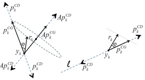
Figure 1: At the 𝑘th iteration of the CG and 𝐶𝐷, the directions 𝑝𝐶𝐺
𝑘 and 𝑝𝐶𝐷𝑘 are
respec-tively generated, along the line ℓ. Applying the CG, the vectors 𝑝𝐶𝐺𝑘 and 𝑟𝑘 have the same
orthogonal projection on 𝐴𝑝𝐶𝐺
𝑘 , since (𝑝𝐶𝐺𝑘 )𝑇𝐴𝑝𝐶𝐺𝑘 = 𝑟𝑘𝑇𝐴𝑝𝐶𝐺𝑘 . Applying 𝐶𝐷, the latter
equality with 𝑝𝐶𝐷
Table 3: The new 𝐶𝐷-red class for solving (1), obtained by setting at Step 𝑘 of 𝐶𝐷 the parameter 𝛾𝑘 as in relation (28).
The 𝐶𝐷-red class Step 0: Set 𝑘 = 0, 𝑦0 ∈ ℝ𝑛, 𝑟0 := 𝑏− 𝐴𝑦0.
If 𝑟0= 0, then STOP. Else, set 𝑝0:= 𝑟0, 𝑘 = 𝑘 + 1.
Compute 𝑎0 := 𝑟0𝑇𝑝0/𝑝0𝑇𝐴𝑝0, 𝛾0:=−𝑎0,
𝑦1 := 𝑦0+ 𝑎0𝑝0, 𝑟1 := 𝑟0− 𝑎0𝐴𝑝0.
If 𝑟1= 0, then STOP. Else, set 𝜎0:= 𝛾0∥𝐴𝑝0∥2/𝑝𝑇0𝐴𝑝0, 𝛽0 =−(1 + 𝜎0)
𝑝1 := 𝑟1+ 𝛽0𝑝0, 𝑘 = 𝑘 + 1.
Step 𝑘: Compute 𝑎𝑘−1 := 𝑟𝑘−1𝑇 𝑝𝑘−1/𝑝𝑇𝑘−1𝐴𝑝𝑘−1,
𝑦𝑘:= 𝑦𝑘−1+ 𝑎𝑘−1𝑝𝑘−1, 𝑟𝑘 := 𝑟𝑘−1− 𝑎𝑘−1𝐴𝑝𝑘−1.
If 𝑟𝑘= 0, then STOP. Else, use (28) to compute 𝛾𝑘−1.
Set 𝜎𝑘−1 := 𝛾𝑘−1 ∥𝐴𝑝𝑘−1∥ 2 𝑝𝑇 𝑘−1𝐴𝑝𝑘−1, 𝛽𝑘−1:=−(1 + 𝜎𝑘−1) 𝑝𝑘:= 𝑟𝑘+ 𝛽𝑘−1𝑝𝑘−1, 𝑘 = 𝑘 + 1. Go to Step 𝑘.
Relations (24)-(25) suggest that the sequence{𝛾𝑘} must satisfy specific conditions in order
to reduce 𝐶𝐷 equivalently to the CG. For a possible generalization of the latter conclusion, consider that equalities (23) are by (5) sufficient conditions in order to reduce 𝐶𝐷 equiv-alently to the CG. Thus, now we want to study general conditions on the sequence {𝛾𝑘},
such that (23) are satisfied. By (23) we have
−(1 + 𝜔𝑘) = 𝜎𝑘−1,
which is equivalent from Table 2 to
−(𝛾𝑘−1∥𝐴𝑝𝑘−1∥2+ 𝑝𝑇𝑘−1𝐴𝑝𝑘−1) = 𝛾𝑘 𝛾𝑘−1 𝑝𝑇𝑘𝐴𝑝𝑘 (26) or −𝛾2𝑘−1∥𝐴𝑝𝑘−1∥2− 𝛾𝑘−1𝑝𝑘−1𝑇 𝐴𝑝𝑘−1− 𝛾𝑘𝑝𝑇𝑘𝐴𝑝𝑘= 0. (27)
The latter equality, for 𝑘≥ 1, and the choice of 𝜎0in Table 2 yield the following conclusions.
Lemma 6.1 [Reduction of 𝐶𝐷] The scheme 𝐶𝐷 in Table 2 can be rewritten as in Table 3 (i.e. with the CG-like structure of Table 1), provided that the sequence {𝛾𝑘} satisfies
𝛾0 :=−𝑎0 and 𝛾𝑘:=− 𝛾𝑘−12 ∥𝐴𝑝𝑘−1∥2+ 𝛾𝑘−1𝑝𝑇𝑘−1𝐴𝑝𝑘−1 𝑝𝑇 𝑘𝐴𝑝𝑘 , 𝑘≥ 1. (28)
Proof
By the considerations which led to (26)-(27), relation (28) yields (23), so that the scheme 𝐶𝐷-red in Table 3 follows from 𝐶𝐷 with the position (28), and setting 𝛾0=−𝑎0.
Furthermore, replacing in (28) the conditions 𝛾𝑖 = −𝑎𝑖, 𝑖 ≥ 1, and recalling (i)-(ii), we
obtain the condition 𝑎2𝑘−1∥𝐴𝑝𝑘−1∥2=∥𝑟𝑘−1∥2+∥𝑟𝑘∥2, which is immediately fulfilled using
condition 𝑟𝑘= 𝑟𝑘−1− 𝑎𝑘−1𝐴𝑝𝑘−1. □
Note that the 𝐶𝐷-red scheme substantially is more similar to the CG than to 𝐶𝐷. Indeed the conditions (8), explicitly imposed at Step 𝑘 of 𝐶𝐷, reduce to the unique condition 𝑝𝑇
𝑘𝐴𝑝𝑘−1 = 0 in 𝐶𝐷-red.
The following result is a trivial consequence of Lemma 4.5, where the alternate use of CG and 𝐶𝐷 steps is analyzed.
Lemma 6.2 [Combined Finite Convergence] Let Assumption 4.1 hold. Let 𝑦1, . . . , 𝑦ℎ
be the iterates generated by 𝐶𝐷, with ℎ ≤ 𝑛 and 𝐴𝑦ℎ = 𝑏. Then, finite convergence is
preserved (i.e. 𝐴𝑦ℎ = 𝑏) if the Step ˆ𝑘 of 𝐶𝐷, with ˆ𝑘∈ {𝑘1, . . . , 𝑘ℎ} ⊆ {1, . . . , ℎ}, is replaced
by the Step ˆ𝑘 of the CG. Proof
First observe that both in Table 1 and Table 2, for any 𝑘 ≤ ℎ, the quantity ∥𝑟𝑘∥ > 0 is
computed. Thus, in Table 1 the coefficient 𝛽𝑘−1 is well defined for any 𝑛 > 𝑘 ≥ 1. Now, by
Table 2, setting at Step ˆ𝑘∈ {𝑘1, . . . , 𝑘ℎ} ⊆ {1, . . . , ℎ} the following
⎧ ⎨ ⎩ 𝛾ˆ𝑘−1=−𝑎ˆ𝑘−1 if ˆ𝑘≥ 1 𝜎ˆ𝑘−1 =−(1 + 𝛽ˆ𝑘−1) if ˆ𝑘≥ 1 𝜔𝑘−1ˆ = 𝛽𝑘−2ˆ if ˆ𝑘≥ 2,
the Step ˆ𝑘 of 𝐶𝐷 coincides formally with the Step ˆ𝑘 of CG. Thus, finite convergence with 𝐴𝑦ℎ = 𝑏 is proved recalling that Lemma 4.5 holds for any choice of the sequence{𝛾𝑘}, with
𝛾𝑘∕= 0. □
7
Relation Between the Scaled-CG and 𝐶𝐷
Similarly to the previous section, here we aim at determining the relation between our proposal in Table 2 and the scheme of the scaled-CG in Table 4 (see also [8], page 125). In [8] a motivated choice for the coefficients {𝜌𝑘} in the scaled-CG is also given. Here,
following the guidelines of the previous section, we first rewrite the relation 𝑝𝑘+1:= 𝜌𝑘+1(𝑟𝑘+1+ 𝛽𝑘𝑝𝑘),
at Step 𝑘 + 1 of the scaled-CG, as follows
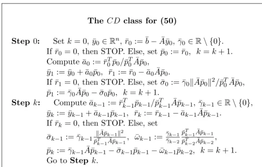
Table 4: The scaled-CG algorithm for solving (1).
The Scaled-CG method Step 0: Set 𝑘 = 0, 𝑦0∈ ℝ, 𝑟0 := 𝑏− 𝐴𝑦0.
If 𝑟0= 0, then STOP. Else, set 𝑝0:= 𝜌0𝑟0, 𝜌0 > 0, 𝑘 = 𝑘 + 1.
Step 𝑘: Compute 𝛼𝑘−1 := 𝜌𝑘−1∥𝑟𝑘−1∥2/𝑝𝑇𝑘−1𝐴𝑝𝑘−1, 𝜌𝑘−1 > 0,
𝑦𝑘:= 𝑦𝑘−1+ 𝛼𝑘−1𝑝𝑘−1, 𝑟𝑘:= 𝑟𝑘−1− 𝛼𝑘−1𝐴𝑝𝑘−1.
If 𝑟𝑘= 0, then STOP. Else, set 𝛽𝑘−1 :=−𝑝𝑇𝑘−1𝐴𝑟𝑘/𝑝𝑇𝑘−1𝐴𝑝𝑘−1 or
𝛽𝑘−1 :=∥𝑟𝑘∥2/(𝜌𝑘−1∥𝑟𝑘−1∥2) 𝑝𝑘:= 𝜌𝑘(𝑟𝑘+ 𝛽𝑘−1𝑝𝑘−1), 𝜌𝑘 > 0, 𝑘 = 𝑘 + 1, Go to Step 𝑘. = 𝜌𝑘+1[ 𝑝𝑘 𝜌𝑘 − 𝛽𝑘−1 𝑝𝑘−1− 𝛼𝑘𝐴𝑝𝑘 ] + 𝜌𝑘+1𝛽𝑘𝑝𝑘 = −𝜌𝑘+1𝛼𝑘𝐴𝑝𝑘+ 𝜌𝑘+1 ( 𝛽𝑘+ 1 𝜌𝑘 ) 𝑝𝑘− 𝜌𝑘+1𝛽𝑘−1𝑝𝑘−1. (29)
We want to show that for a suitable choice of the parameters {𝛾𝑘}, the 𝐶𝐷 yields the
recursion (29) of the scaled-CG, i.e. for a proper choice of {𝛾𝑘} we obtain from CD a
scheme equivalent to the scaled-CG. On this purpose let us set in 𝐶𝐷
𝛾𝑘=−𝜌𝑘+1𝛼𝑘, 𝑘≥ 0, (30)
where 𝛼𝑘 is given at Step 𝑘 of Table 4. Thus, by Table 2
𝜎𝑘 = 𝛾𝑘∥𝐴𝑝𝑘∥ 2 𝑝𝑇 𝑘𝐴𝑝𝑘 = −𝜌𝑘+1𝛼𝑘∥𝐴𝑝𝑘∥ 2 𝑝𝑇 𝑘𝐴𝑝𝑘 , 𝑘≥ 0, (31) and for 𝑘≥ 1 𝜔𝑘 = 𝛾𝑘 𝛾𝑘−1 𝑝𝑇 𝑘𝐴𝑝𝑘 𝑝𝑇 𝑘−1𝐴𝑝𝑘−1 = 𝜌𝑘+1𝛼𝑘 𝜌𝑘𝛼𝑘−1 𝑝𝑇 𝑘𝐴𝑝𝑘 𝑝𝑇 𝑘−1𝐴𝑝𝑘−1 . (32)
Now, comparing the coefficients in (29) with (30), (31) and (32), we want to prove that the choice (30) implies 𝜎𝑘 = −𝜌𝑘+1 ( 𝛽𝑘+ 1 𝜌𝑘 ) , 𝑘≥ 0, (33) 𝜔𝑘 = 𝜌𝑘+1𝛽𝑘−1, 𝑘≥ 1, (34)
As regards (33), from Table 4 we have for 𝑘 ≥ 0 𝛽𝑘+ 1 𝜌𝑘 = 1 𝜌𝑘𝑝 𝑇 𝑘𝐴𝑝𝑘− 𝑟𝑘+1𝑇 𝐴𝑝𝑘 𝑝𝑇 𝑘𝐴𝑝𝑘 = ( 1 𝜌𝑘𝑝𝑘− 𝑟𝑘+1 )𝑇 𝐴𝑝𝑘 𝑝𝑇 𝑘𝐴𝑝𝑘 = ( 1 𝜌𝑘𝑝𝑘− 𝑟𝑘+ 𝛼𝑘𝐴𝑝𝑘 )𝑇 𝐴𝑝𝑘 𝑝𝑇 𝑘𝐴𝑝𝑘 = (𝑟𝑘+ 𝛽𝑘−1𝑝𝑘−1− 𝑟𝑘+ 𝛼𝑘𝐴𝑝𝑘) 𝑇 𝐴𝑝𝑘 𝑝𝑇 𝑘𝐴𝑝𝑘 = 𝛼𝑘∥𝐴𝑝𝑘∥ 2 𝑝𝑇 𝑘𝐴𝑝𝑘 ,
so that from (31) the condition (33) holds, for any 𝑘 ≥ 0. As regards (34) from Step 𝑘 of Table 4 we know that 𝛽𝑘−1 = ∥𝑟𝑘∥2/(𝜌𝑘−1∥𝑟𝑘−1∥2) and, since 𝑟𝑇𝑘𝑝𝑘−1 = 0, we obtain
𝑟𝑇
𝑘𝑝𝑘= 𝜌𝑘∥𝑟𝑘∥2; thus, relation (30) yields
𝛽𝑘−1 = ∥𝑟𝑘∥ 2 𝜌𝑘−1∥𝑟𝑘−1∥2 = 𝛼𝑘 𝜌𝑘𝛼𝑘−1 𝑝𝑇𝑘𝐴𝑝𝑘 𝑝𝑇 𝑘−1𝐴𝑝𝑘−1 = 𝛾𝑘 𝜌𝑘+1𝛾𝑘−1 𝑝𝑇𝑘𝐴𝑝𝑘 𝑝𝑇 𝑘−1𝐴𝑝𝑘−1 , 𝑘≥ 1. Relation (34) is proved using the latter equality and (32).
8
Matrix Factorization Induced by 𝐶𝐷
We first recall that considering the CG in Table 1 and setting at Step ℎ 𝑃ℎ := ( 𝑝0 ∥𝑟0∥ ⋅ ⋅ ⋅ 𝑝ℎ ∥𝑟ℎ∥ ) 𝑅ℎ := ( 𝑟0 ∥𝑟0∥ ⋅ ⋅ ⋅ 𝑟ℎ ∥𝑟ℎ∥ ) , along with 𝐿ℎ:= ⎛ ⎜ ⎜ ⎜ ⎜ ⎜ ⎜ ⎜ ⎜ ⎜ ⎜ ⎜ ⎜ ⎜ ⎝ 1 −√𝛽0 1 −√𝛽1 1 . .. 1 −√𝛽ℎ−1 1 ⎞ ⎟ ⎟ ⎟ ⎟ ⎟ ⎟ ⎟ ⎟ ⎟ ⎟ ⎟ ⎟ ⎟ ⎠ ∈ ℝℎ×ℎ
and 𝐷ℎ := diag𝑖{1/𝛼𝑖}, we obtain the three matrix relations
𝑃ℎ𝐿𝑇ℎ = 𝑅ℎ (35) 𝐴𝑃ℎ = 𝑅ℎ𝐿ℎ𝐷ℎ− √ 𝛽ℎ 𝛼ℎ 𝑟ℎ+1 ∥𝑟ℎ+1∥ 𝑒𝑇ℎ (36) 𝑅𝑇ℎ𝐴𝑅ℎ = 𝑇ℎ = 𝐿ℎ𝐷ℎ𝐿𝑇ℎ. (37)
Then, in this section we are going to use the iteration in Table 2 in order to possibly recast relations (35)-(37) for 𝐶𝐷.
On this purpose, from Table 2 we can easily draw the following relation between the sequences{𝑝0, 𝑝1, . . .} and {𝑟0, 𝑟1, . . .} 𝑝0 = 𝑟0 𝑝1 = 𝛾0 𝑎0 (𝑟0− 𝑟1)− 𝜎0𝑝0 𝑝𝑖 = 𝛾𝑖−1 𝑎𝑖−1 (𝑟𝑖−1− 𝑟𝑖)− 𝜎𝑖−1𝑝𝑖−1− 𝜔𝑖−1𝑝𝑖−2, 𝑖 = 2, 3, . . . ,
and introducing the positions
𝑃ℎ := (𝑝0 𝑝1 ⋅ ⋅ ⋅ 𝑝ℎ) 𝑅ℎ := (𝑟0 𝑟1 ⋅ ⋅ ⋅ 𝑟ℎ) ¯ 𝑅ℎ := ( 𝑟0 ∥𝑟0∥ ⋅ ⋅ ⋅ 𝑟ℎ ∥𝑟ℎ∥ ) , along with the matrices
𝑈ℎ,1:= ⎛ ⎜ ⎜ ⎜ ⎜ ⎜ ⎜ ⎜ ⎜ ⎜ ⎜ ⎜ ⎜ ⎝ 1 𝜎0 𝜔1 0 ⋅ ⋅ ⋅ ⋅ ⋅ ⋅ 0 1 𝜎1 𝜔2 0 ⋅ ⋅ ⋅ 0 1 𝜎2 . .. 0 ... 1 . .. ... 0 . .. ... 𝜔ℎ−1 . .. 𝜎ℎ−1 1 ⎞ ⎟ ⎟ ⎟ ⎟ ⎟ ⎟ ⎟ ⎟ ⎟ ⎟ ⎟ ⎟ ⎠ ∈ ℝ(ℎ+1)×(ℎ+1), 𝑈ℎ,2 := ⎛ ⎜ ⎜ ⎜ ⎜ ⎜ ⎜ ⎜ ⎜ ⎜ ⎜ ⎜ ⎜ ⎜ ⎜ ⎜ ⎜ ⎜ ⎜ ⎝ ∥𝑟0∥ ∥𝑟0∥ 0 ⋅ ⋅ ⋅ ⋅ ⋅ ⋅ 0 −∥𝑟1∥ ∥𝑟1∥ 0 ⋅ ⋅ ⋅ 0 −∥𝑟2∥ ∥𝑟2∥ 0 ... . .. . .. 0 −∥𝑟ℎ−1∥ ∥𝑟ℎ−1∥ −∥𝑟ℎ∥ ⎞ ⎟ ⎟ ⎟ ⎟ ⎟ ⎟ ⎟ ⎟ ⎟ ⎟ ⎟ ⎟ ⎟ ⎟ ⎟ ⎟ ⎟ ⎟ ⎠ ∈ ℝ(ℎ+1)×(ℎ+1)
and 𝐷ℎ := diag { 1 , diag 𝑖=0,...,ℎ−1{𝛾𝑖/𝑎𝑖} } ∈ ℝ(ℎ+1)×(ℎ+1), we obtain after ℎ− 1 iterations of 𝐶𝐷
𝑃ℎ𝑈ℎ,1= ¯𝑅ℎ𝑈ℎ,2𝐷ℎ,
so that
𝑃ℎ = ¯𝑅ℎ𝑈ℎ,2𝐷ℎ𝑈ℎ,1−1 = ¯𝑅ℎ𝑈ℎ,
where 𝑈ℎ = 𝑈ℎ,2𝐷ℎ𝑈ℎ,1−1. Now, observe that 𝑈ℎ is upper triangular since 𝑈ℎ,2 is upper
bidiagonal, 𝐷ℎ is diagonal and 𝑈ℎ,1−1 may be easily seen to be upper triangular. As a
consequence, recalling that 𝑝0, . . . , 𝑝ℎ are mutually conjugate we have
¯
𝑅𝑇ℎ𝐴 ¯𝑅ℎ = 𝑈ℎ−𝑇diag𝑖{𝑝𝑇𝑖 𝐴𝑝𝑖}𝑈ℎ−1,
and in case ℎ = 𝑛− 1, again from the conjugacy of 𝑝0, . . . , 𝑝𝑛−1
𝑃𝑛−1𝑇 𝐴𝑃𝑛−1= 𝑈𝑛−1𝑇 𝑅¯𝑇𝑛−1𝐴 ¯𝑅𝑛−1𝑈𝑛−1= diag
𝑖=0,...,ℎ−1{𝑝
𝑇 𝑖 𝐴𝑝𝑖}.
From the orthogonality of ¯𝑅𝑛−1, along with relation
det(𝑈𝑛−1) =∥𝑟0∥ 𝑛−1 ∏ 𝑗=1 ( −∥𝑟𝑎𝑗∥𝛾𝑗−1 𝑗−1 ) = (𝑛−1 ∏ 𝑖=0 ∥𝑟𝑖∥ ) (𝑛−2 ∏ 𝑖=0 −𝛾𝑎𝑖 𝑖 ) , we have det(𝑈𝑇 𝑛−1𝑅¯𝑇𝑛−1𝐴 ¯𝑅𝑛−1𝑈𝑛−1) = 𝑛−1 ∏ 𝑖=0 𝑝𝑇𝑖 𝐴𝑝𝑖 ⇐⇒ det(𝐴) = 𝑛−1 ∏ 𝑖=0 𝑝𝑇𝑖 𝐴𝑝𝑖 det(𝑈𝑛−1)2 . Thus, in the end
det(𝐴) = [𝑛−1 ∏ 𝑖=0 𝑝𝑇 𝑖 𝐴𝑝𝑖 ∥𝑟𝑖∥2 ] ⋅ [𝑛−2 ∏ 𝑖=0 𝑎2𝑖 ] [𝑛−2 ∏ 𝑖=0 𝛾𝑖2 ] . (38)
Note that the following considerations hold:
∙ for 𝛾𝑖 = ±𝑎𝑖 (which includes the case 𝛾𝑖 = −𝑎𝑖, when by Lemma 6.1 𝐶𝐷 reduces
equivalently to the CG), by (i) of Section 6 ∣𝑝𝑇
𝑘𝑟𝑘∣ = ∥𝑟𝑘∥2, so that we obtain the
standard result (see also [14]) det(𝐴) = [𝑛−1 ∏ 𝑖=0 𝑝𝑇 𝑖𝐴𝑝𝑖 ∥𝑟𝑖∥2 ] = 𝑛−1 ∏ 𝑖=0 1 𝑎𝑖 ;
9
Issues on the Conjugacy Loss for 𝐶𝐷
Here we consider a simplified approach to describe the conjugacy loss for both the CG and 𝐶𝐷, under Assumption 4.1 (see also [14] for a similar approach). Suppose that both the CG and 𝐶𝐷 perform Step 𝑘 + 1, and for numerical reasons a nonzero conjugacy error 𝜀𝑘,𝑗
respectively occurs between directions 𝑝𝑘 and 𝑝𝑗, i.e.
𝜀𝑘,𝑗 := 𝑝𝑇𝑘𝐴𝑝𝑗 ∕= 0, 𝑗≤ 𝑘 − 1.
Then, we calculate the conjugacy error
𝜀𝑘+1,𝑗 = 𝑝𝑇𝑘+1𝐴𝑝𝑗, 𝑗≤ 𝑘,
for both the CG and 𝐶𝐷. First observe that at Step 𝑘 + 1 of Table 1 we have
𝜀𝑘+1,𝑗 = (𝑟𝑘+1+ 𝛽𝑘𝑝𝑘)𝑇𝐴𝑝𝑗 (39)
= (𝑝𝑘− 𝛽𝑘−1𝑝𝑘−1− 𝛼𝑘𝐴𝑝𝑘)𝑇 𝐴𝑝𝑗 + 𝛽𝑘𝜀𝑘,𝑗 (40)
= (1 + 𝛽𝑘)𝜀𝑘,𝑗− 𝛽𝑘−1𝜀𝑘−1,𝑗− 𝛼𝑘(𝐴𝑝𝑘)𝑇𝐴𝑝𝑗. (41)
Then, from relation 𝐴𝑝𝑗 = (𝑟𝑗 − 𝑟𝑗+1)/𝛼𝑗 and relations (2)-(3) we have for the CG
(𝐴𝑝𝑘)𝑇𝐴𝑝𝑗 = ⎧ ⎨ ⎩ −𝑝 𝑇 𝑘𝐴𝑝𝑘 𝛼𝑘−1 , 𝑗 = 𝑘− 1, ∅, 𝑗≤ 𝑘 − 2.
Thus, observing that for the CG we have 𝜀𝑖,𝑖−1 = 0 and 𝜀𝑖,𝑖 = 𝑝𝑇𝑖𝐴𝑝𝑖, 1≤ 𝑖 ≤ 𝑘 + 1, after
some computation we obtain from (2), (3) and (41)
𝜀𝑘+1,𝑗 = ⎧ ⎨ ⎩ ∅, 𝑗 = 𝑘, ∅, 𝑗 = 𝑘− 1, (1 + 𝛽𝑘)𝜀𝑘,𝑘−2, 𝑗 = 𝑘− 2, (1 + 𝛽𝑘)𝜀𝑘,𝑗− 𝛽𝑘−1𝜀𝑘−1,𝑗− Σ𝑘𝑗, 𝑗≤ 𝑘 − 3, (42)
where Σ𝑘𝑗 ∈ ℝ summarizes the contribution of the term 𝛼𝑘(𝐴𝑝𝑘)𝑇𝐴𝑝𝑗, due to a possible
conjugacy loss.
Let us consider now for 𝐶𝐷 a result similar to (42). We obtain the following relations for 𝑗≤ 𝑘
= 𝛾𝑘(𝐴𝑝𝑘)𝑇𝐴𝑝𝑗− 𝜎𝑘𝜀𝑘,𝑗− 𝜔𝑘𝜀𝑘−1,𝑗 = 𝛾𝑘 𝛾𝑗 (𝐴𝑝𝑘)𝑇 (𝑝𝑗+1+ 𝜎𝑗𝑝𝑗+ 𝜔𝑗𝑝𝑗−1)− 𝜎𝑘𝜀𝑘,𝑗− 𝜔𝑘𝜀𝑘−1,𝑗 = 𝛾𝑘 𝛾𝑗 𝜀𝑘,𝑗+1+( 𝛾𝑘 𝛾𝑗 𝜎𝑗− 𝜎𝑘 ) 𝜀𝑘,𝑗+ 𝛾𝑘 𝛾𝑗 𝜔𝑗𝜀𝑘,𝑗−1− 𝜔𝑘𝜀𝑘−1,𝑗,
and considering now relations (8), the conjugacy among directions 𝑝0, 𝑝1, . . . , 𝑝𝑘 satisfies
𝜀ℎ,𝑙 = 𝑝𝑇ℎ𝐴𝑝𝑙 = 0, for any ∣ ℎ − 𝑙 ∣ ∈ {1, 2}. (43)
Thus, relation (10) and the expression of the coefficients in 𝐶𝐷 yields for 𝜀𝑘+1,𝑗 the
expres-sion ⎧ ⎨ ⎩ ∅, 𝑗 = 𝑘, ∅, 𝑗 = 𝑘− 1, 𝛾𝑘 𝛾𝑘−2 𝜔𝑘−2𝜀𝑘,𝑘−3, 𝑗 = 𝑘− 2, ( 𝛾𝑘 𝛾𝑘−3 𝜎𝑘−3− 𝜎𝑘 ) 𝜀𝑘,𝑘−3+ 𝛾𝑘 𝛾𝑘−3 𝜔𝑘−3𝜀𝑘,𝑘−4, 𝑗 = 𝑘− 3, 𝛾𝑘 𝛾𝑗 𝜀𝑘,𝑗+1+( 𝛾𝑘 𝛾𝑗 𝜎𝑗− 𝜎𝑘 ) 𝜀𝑘,𝑗+ 𝛾𝑘 𝛾𝑗 𝜔𝑗𝜀𝑘,𝑗−1− 𝜔𝑘𝜀𝑘−1,𝑗, 𝑗≤ 𝑘 − 4. (44)
Finally, comparing relations (42) and (44) we have
∙ in case 𝑗 = 𝑘 − 2 the conjugacy error 𝜀𝑘+1,𝑘−2 is nonzero for both the CG and 𝐶𝐷,
as expected. However, for the CG
∣𝜀𝑘+1,𝑘−2∣ > ∣𝜀𝑘,𝑘−2∣
since (1 + 𝛽𝑘) > 1, which theoretically can lead to an harmful amplification of
con-jugacy errors. On the contrary, for 𝐶𝐷 the positive quantity ∣𝛾𝑘𝜔𝑘−2/𝛾𝑘−2∣ in the
expression of 𝜀𝑘+1,𝑘−2 can be possibly smaller than one.
∙ choosing the sequence {𝛾𝑘} such that
𝛾𝑘 𝛾𝑘−𝑖 ≪ 1 and/or 𝛾𝑘 𝛾𝑘−𝑖 𝜔𝑘−𝑖 ≪ 1, 𝑖 = 2, 3, . . . (45) from (44) the effects of conjugacy loss may be attenuated. Thus, a strategy to update the sequence{𝛾𝑘} so that (45) holds might be investigated.
9.1 Bounds for the Coefficients of 𝐶𝐷
We want to describe here the sensitivity of the coefficients 𝜎𝑘and 𝜔𝑘, at Step 𝑘 + 1 of 𝐶𝐷,
to the condition number 𝜅(𝐴). In particular, we want to provide a comparison with the CG, in order to identify possible advantages/disadvantages of our proposal. From Table 2 and Assumption 4.1 we have
∣𝜔𝑘∣ = 𝛾𝑘 𝛾𝑘−1 𝑝𝑇𝑘𝐴𝑝𝑘 𝑝𝑇 𝑘−1𝐴𝑝𝑘−1 , ∣𝜎𝑘∣ = 𝛾𝑘∥𝐴𝑝𝑘∥ 2 𝑝𝑇 𝑘𝐴𝑝𝑘 , so that ⎧ ⎨ ⎩ ∣𝜔𝑘∣ ≥ 𝛾𝑘 𝛾𝑘−1 𝜆𝑚(𝐴)∥𝑝𝑘∥2 𝜆𝑀(𝐴)∥𝑝𝑘−1∥2 = 𝛾𝑘 𝛾𝑘−1 1 𝜅(𝐴) ∥𝑝𝑘∥2 ∥𝑝𝑘−1∥2 ∣𝜔𝑘∣ ≤ 𝛾𝑘 𝛾𝑘−1 𝜆𝑀(𝐴)∥𝑝𝑘∥2 𝜆𝑚(𝐴)∥𝑝𝑘−1∥2 = 𝛾𝑘 𝛾𝑘−1 𝜅(𝐴) ∥𝑝𝑘∥ 2 ∥𝑝𝑘−1∥2 , (46) and ⎧ ⎨ ⎩ ∣𝜎𝑘∣ ≥ ∣𝛾𝑘∣ 𝜆2 𝑚(𝐴)∥𝑝𝑘∥2 𝜆𝑀(𝐴)∥𝑝𝑘∥2 =∣𝛾𝑘∣ 𝜆𝑚(𝐴) 𝜅(𝐴) ∣𝜎𝑘∣ ≤ ∣𝛾𝑘∣ 𝜆2𝑀(𝐴)∥𝑝𝑘∥2 𝜆𝑚(𝐴)∥𝑝𝑘∥2 =∣𝛾𝑘∣𝜆𝑀(𝐴)𝜅(𝐴). (47)
On the other hand, from Table 1 we obtain for the CG 𝛽𝑘 = − 𝑟𝑇 𝑘+1𝐴𝑝𝑘 𝑝𝑇 𝑘𝐴𝑝𝑘 = −1 + 𝛼𝑘∥𝐴𝑝𝑘∥ 2 𝑝𝑇 𝑘𝐴𝑝𝑘 = − 1 + ∥𝑟𝑘∥ 2 𝑝𝑇 𝑘𝐴𝑝𝑘 ∥𝐴𝑝𝑘∥2 𝑝𝑇 𝑘𝐴𝑝𝑘 ,
so that, since 𝛽𝑘 > 0 and using relation ∥𝑟𝑘∥ ≤ ∥𝑝𝑘∥, along with 𝑝𝑘𝑇𝐴𝑝𝑘 = 𝑟𝑘𝑇𝐴𝑟𝑘 − ∥𝑟𝑘∥4 ∥𝑟𝑘−1∥4𝑝 𝑇 𝑘−1𝐴𝑝𝑘−1> 0, we have ⎧ ⎨ ⎩ 𝛽𝑘 ≥ max { 0,−1 + ∥𝑟𝑘∥ 2 𝑟𝑇 𝑘𝐴𝑟𝑘 𝜆𝑚(𝐴) 𝜅(𝐴) } ≥ max { 0,−1 + 1 [𝜅(𝐴)]2 } = 0 𝛽𝑘 ≤ −1 + ∥𝑝𝑘∥ 2 𝑝𝑇 𝑘𝐴𝑝𝑘 𝜆𝑀(𝐴)𝜅(𝐴)≤ −1 + [𝜅(𝐴)]2. (48)
In particular, this seems to indicate that on those problems where the quantity∣𝛾𝑘∣𝜆𝑀(𝐴)
is reasonably small, 𝐶𝐷 might be competitive. However, as expected, high values for 𝜅(𝐴) may determine numerical instability for both the CG and 𝐶𝐷. In addition, observe that any conclusion on the comparison between the numerical performance of the CG and 𝐶𝐷, depends both on the sequence{𝛾𝑘} and on how tight are the bounds (47) and (48) for the
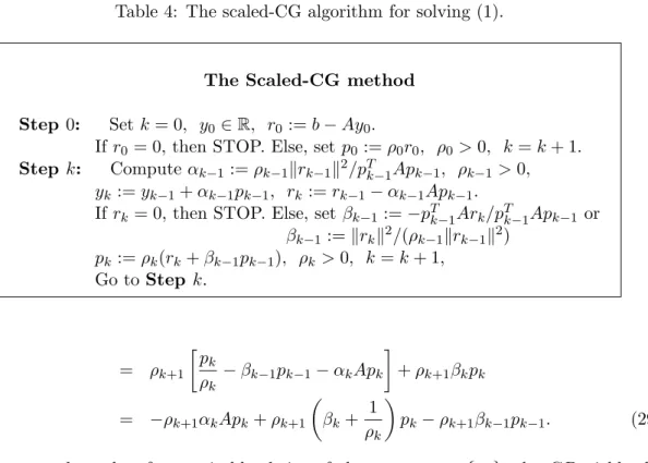
Table 5: The 𝐶𝐷 class for solving the linear system ¯𝐴¯𝑦 = ¯𝑏 in (50).
The 𝐶𝐷 class for (50)
Step 0: Set 𝑘 = 0, ¯𝑦0∈ ℝ𝑛, ¯𝑟0 := ¯𝑏− ¯𝐴¯𝑦0, ¯𝛾0∈ ℝ ∖ {0}.
If ¯𝑟0 = 0, then STOP. Else, set ¯𝑝0 := ¯𝑟0, 𝑘 = 𝑘 + 1.
Compute ¯𝑎0 := ¯𝑟𝑇0𝑝¯0/¯𝑝𝑇0𝐴¯¯𝑝0,
¯
𝑦1 := ¯𝑦0+ ¯𝑎0𝑝¯0, ¯𝑟1:= ¯𝑟0− ¯𝑎0𝐴¯¯𝑝0.
If ¯𝑟1 = 0, then STOP. Else, set ¯𝜎0 := ¯𝛾0∥ ¯𝐴¯𝑝0∥2/¯𝑝𝑇0𝐴¯¯𝑝0,
¯
𝑝1:= ¯𝛾0𝐴¯¯𝑝0− ¯𝜎0𝑝¯0, 𝑘 = 𝑘 + 1.
Step 𝑘: Compute ¯𝑎𝑘−1:= ¯𝑟𝑘−1𝑇 𝑝¯𝑘−1/¯𝑝𝑇𝑘−1𝐴¯¯𝑝𝑘−1, ¯𝛾𝑘−1∈ ℝ ∖ {0},
¯
𝑦𝑘:= ¯𝑦𝑘−1+ ¯𝑎𝑘−1𝑝¯𝑘−1, ¯𝑟𝑘:= ¯𝑟𝑘−1− ¯𝑎𝑘−1𝐴¯¯𝑝𝑘−1.
If ¯𝑟𝑘= 0, then STOP. Else, set
¯ 𝜎𝑘−1:= ¯𝛾𝑘−1 ∥ ¯𝐴¯𝑝𝑘−1∥ 2 ¯ 𝑝𝑇 𝑘−1𝐴¯¯𝑝𝑘−1, ¯𝜔𝑘−1:= ¯ 𝛾𝑘−1 ¯ 𝛾𝑘−2 ¯ 𝑝𝑇 𝑘−1𝐴¯¯𝑝𝑘−1 ¯ 𝑝𝑇 𝑘−2𝐴¯¯𝑝𝑘−2, ¯ 𝑝𝑘:= ¯𝛾𝑘−1𝐴¯¯𝑝𝑘−1− ¯𝜎𝑘−1𝑝¯𝑘−1− ¯𝜔𝑘−1𝑝¯𝑘−2, 𝑘 = 𝑘 + 1. Go to Step 𝑘.
Table 6: The preconditioned 𝐶𝐷, namely 𝐶𝐷ℳ, for solving (1).
The 𝐶𝐷ℳ class
Step 0: Set 𝑘 = 0, 𝑦0∈ ℝ𝑛, 𝑟0 := 𝑏− 𝐴𝑦0, ¯𝛾0∈ ℝ ∖ {0}, ℳ ≻ 0.
If 𝑟0 = 0, then STOP. Else, set 𝑝0 :=ℳ𝑟0, 𝑘 = 𝑘 + 1.
Compute 𝑎0:= 𝑟𝑇0𝑝0/𝑝𝑇0𝐴𝑝0,
𝑦1:= 𝑦0+ 𝑎0𝑝0, 𝑟1:= 𝑟0− 𝑎0𝐴𝑝0.
If 𝑟1 = 0, then STOP. Else, set 𝜎0 := ¯𝛾0∥𝐴𝑝0∥2ℳ/𝑝𝑇0𝐴𝑝0,
𝑝1:= ¯𝛾0ℳ(𝐴𝑝0)− 𝜎0𝑝0, 𝑘 = 𝑘 + 1.
Step 𝑘: Compute 𝑎𝑘−1:= 𝑟𝑘−1𝑇 𝑝𝑘−1/𝑝𝑇𝑘−1𝐴𝑝𝑘−1, ¯𝛾𝑘−1 ∈ ℝ ∖ {0},
𝑦𝑘:= 𝑦𝑘−1+ 𝑎𝑘−1𝑝𝑘−1, 𝑟𝑘:= 𝑟𝑘−1− 𝑎𝑘−1𝐴𝑝𝑘−1.
If 𝑟𝑘= 0, then STOP. Else, set
𝜎𝑘−1:= ¯𝛾𝑘−1∥𝐴𝑝𝑘−1∥ 2 ℳ 𝑝𝑇 𝑘−1𝐴𝑝𝑘−1 , 𝜔𝑘−1:= ¯𝛾¯𝛾𝑘−1𝑘−2 𝑝𝑇 𝑘−1𝐴𝑝𝑘−1 𝑝𝑇 𝑘−2𝐴𝑝𝑘−2 , 𝑝𝑘:= ¯𝛾𝑘−1ℳ(𝐴𝑝𝑘−1)− 𝜎𝑘−1𝑝𝑘−1− 𝜔𝑘−1𝑝𝑘−2, 𝑘 = 𝑘 + 1. Go to Step 𝑘.
10
The Preconditioned 𝐶𝐷 Class
In this section we introduce preconditioning for the class 𝐶𝐷, in order to better cope with possible illconditioning of the matrix 𝐴 in (1).
Let 𝑀 ∈ ℝ𝑛×𝑛 be nonsingular and consider the linear system (1). Since we have
𝐴𝑦 = 𝑏 ⇐⇒ (𝑀𝑇𝑀)−1 𝐴𝑦 =(𝑀𝑇𝑀)−1 𝑏 (49) ⇐⇒ (𝑀−𝑇𝐴𝑀−1) 𝑀𝑦 = 𝑀−𝑇𝑏 ⇐⇒ ¯𝐴¯𝑦 = ¯𝑏, (50) where ¯ 𝐴 := 𝑀−𝑇𝐴𝑀−1, 𝑦 := 𝑀 𝑦,¯ ¯𝑏 := 𝑀−𝑇𝑏, (51)
solving (1) is equivalent to solve (49) or (50). Moreover, any eigenvalue 𝜆𝑖, 𝑖 = 1, . . . , 𝑛,
of 𝑀−𝑇𝐴𝑀−1 is also an eigenvalue of (𝑀𝑇𝑀)−1 𝐴. Indeed, if (𝑀𝑇𝑀 )−1𝐴𝑧 𝑖 = 𝜆𝑖𝑧𝑖, 𝑖 = 1, . . . , 𝑛, then (𝑀−1𝑀−𝑇) 𝐴𝑀−1(𝑀 𝑧 𝑖) = 𝜆𝑖𝑧𝑖 so that 𝑀−𝑇𝐴𝑀−1(𝑀 𝑧𝑖) = 𝜆𝑖(𝑀 𝑧𝑖) .
Now, let us motivate the importance of selecting a promising matrix 𝑀 in (50), in order to reduce 𝜅( ¯𝐴) (or equivalently to reduce 𝜅[(𝑀𝑇𝑀 )−1𝐴]).
Observe that under the Assumption 4.1 and using standard Chebyshev polynomials analysis, we can prove that in exact algebra for both the CG and 𝐶𝐷 the following relation holds (see [2] for details, and a similar analysis holds for 𝐶𝐷)
∥𝑦𝑘− 𝑦∗∥𝐴 ∥𝑦0− 𝑦∗∥𝐴 ≤ 2 ( √ 𝜅(𝐴)− 1 √𝜅(𝐴) + 1 )𝑘 , (52)
where 𝐴𝑦∗ = 𝑏. Relation (52) reveals the strong dependency of the iterates generated by the CG and 𝐶𝐷, on 𝜅(𝐴). In addition, if the CG and 𝐶𝐷 are used to solve (50) in place of (1), then the bound (52) becomes
∥𝑦𝑘− 𝑦∗∥𝐴 ∥𝑦0− 𝑦∗∥𝐴 ≤ 2 ( √ 𝜅[(𝑀𝑇𝑀 )−1𝐴]− 1 √𝜅[(𝑀𝑇𝑀 )−1𝐴] + 1 )𝑘 , (53)
which encourages to use the preconditioner (𝑀𝑇𝑀 )−1 when 𝜅[(𝑀𝑇𝑀 )−1𝐴] < 𝜅(𝐴).
On this guideline we want to introduce preconditioning in our scheme 𝐶𝐷, for solving the linear system (50), where 𝑀 is non-singular. We do not expect that necessarily when 𝑀 = 𝐼 (i.e. no preconditioning is considered in (50)) 𝐶𝐷 outperforms the CG. Indeed, as stated in the previous section, 𝑀 = 𝐼 along with bounds (46), (47) and (48) do not suggest a specific preference for 𝐶𝐷 with respect to the CG. On the contrary, suppose a suitable preconditioner ℳ = (𝑀𝑇𝑀 )−1 is selected when 𝜅(𝐴) is large. Then, since the class 𝐶𝐷
respect to the CG, it may possibly better recover the conjugacy loss.
We will soon see that if the preconditioner ℳ is adopted in 𝐶𝐷, it is just used throughout the computation of the productℳ × 𝑣, 𝑣 ∈ ℝ𝑛, i.e. it is not necessary to store the possibly
dense matrix ℳ.
The algorithms in 𝐶𝐷 for (50) are described in Table 5, where each ‘bar’ quantity has a corresponding quantity in Table 2. Then, after substituting in Table 5 the positions
¯ 𝑦𝑘 := 𝑀 𝑦𝑘 ¯ 𝑝𝑘 := 𝑀 𝑝𝑘 ¯ 𝑟𝑘 := 𝑀−𝑇𝑟𝑘 ℳ := (𝑀𝑇𝑀)−1 , (54)
the vector ¯𝑝𝑘 becomes
¯ 𝑝𝑘 = 𝑀 𝑝𝑘= ¯𝛾𝑘−1𝑀−𝑇𝐴𝑀−1𝑀 𝑝𝑘−1− ¯𝜎𝑘−1𝑀 𝑝𝑘−1− ¯𝜔𝑘−1𝑀 𝑝𝑘−2, hence 𝑝𝑘= ¯𝛾𝑘−1ℳ𝐴𝑝𝑘−1− ¯𝜎𝑘−1𝑝𝑘−1− ¯𝜔𝑘−1𝑝𝑘−2 with ¯ 𝜎𝑘−1 = ¯𝛾𝑘−1∥𝑀 −𝑇𝐴𝑝 𝑘−1∥2 𝑝𝑇 𝑘−1𝐴𝑝𝑘−1 = ¯𝛾𝑘−1 (𝐴𝑝𝑘−1)𝑇ℳ𝐴𝑝𝑘−1 𝑝𝑇 𝑘−1𝐴𝑝𝑘−1 (55) ¯ 𝜔𝑘−1 = ¯ 𝛾𝑘−1 ¯ 𝛾𝑘−2 𝑝𝑇𝑘−1𝑀𝑇𝑀−𝑇𝐴𝑀−1𝑀 𝑝𝑘−1 𝑝𝑇 𝑘−2𝑀𝑇𝑀−𝑇𝐴𝑀−1𝑀 𝑝𝑘−2 = 𝛾¯𝑘−1 ¯ 𝛾𝑘−2 𝑝𝑇𝑘−1𝐴𝑝𝑘−1 𝑝𝑇 𝑘−2𝐴𝑝𝑘−2 . Moreover, relation ¯𝑟0= ¯𝑏− ¯𝐴¯𝑦0 becomes
𝑀−𝑇𝑟0 = 𝑀−𝑇𝑏− 𝑀−𝑇𝐴𝑀−1𝑀 𝑦0 ⇐⇒ 𝑟0 = 𝑏− 𝐴𝑦0,
and since ¯𝑝0 = 𝑀 𝑝0 = ¯𝑟0 = 𝑀−𝑇𝑟0 then 𝑝0 = ℳ𝑟0, so that the coefficients ¯𝜎0 and ¯𝑎0
become ¯ 𝜎0 = ¯𝛾0 𝑝𝑇0𝑀𝑇𝑀−𝑇𝐴𝑀−1𝑀−𝑇𝐴𝑀−1𝑀 𝑝0 𝑝𝑇 0𝐴𝑝0 = ¯𝛾0 (𝐴𝑝0)𝑇ℳ(𝐴𝑝0) 𝑝𝑇 0𝐴𝑝0 = ¯𝛾0∥𝐴𝑝0∥ 2 ℳ 𝑝𝑇 0𝐴𝑝0 (56) ¯ 𝑎0 = 𝑟𝑇 0𝑀−1𝑀 𝑝0 𝑝𝑇 0𝑀𝑇𝑀−𝑇𝐴𝑀−1𝑀 𝑝0 = 𝑟 𝑇 0𝑝0 𝑝𝑇 0𝐴𝑝0 . As regards relation ¯𝑝1= ¯𝛾0𝐴¯¯𝑝0− ¯𝜎0𝑝¯0 we have
𝑀 𝑝1 = ¯𝛾0𝑀−𝑇𝐴𝑀−1𝑀 𝑝0− ¯𝜎0𝑀 𝑝0,
hence
Finally, ¯𝑟𝑘= 𝑀−𝑇𝑟𝑘 so that ¯ 𝑟𝑘= 𝑀−𝑇𝑟𝑘= 𝑀−𝑇𝑟𝑘−1− ¯𝑎𝑘−1𝑀−𝑇𝐴𝑀−1𝑀 𝑝𝑘−1 and therefore 𝑟𝑘 = 𝑟𝑘−1− ¯𝑎𝑘−1𝐴𝑝𝑘−1, with ¯ 𝑎𝑘−1 = 𝑟𝑇 𝑘−1𝑀−1𝑀 𝑝𝑘−1 𝑝𝑇 𝑘−1𝑀𝑇𝑀−𝑇𝐴𝑀−1𝑀 𝑝𝑘−1 = 𝑟 𝑇 𝑘−1𝑝𝑘−1 𝑝𝑇 𝑘−1𝐴𝑝𝑘−1 .
The overall resulting preconditioned algorithm 𝐶𝐷ℳ is detailed in Table 6. Observe that
the coefficients 𝑎𝑘−1 and 𝜔𝑘−1 in Tables 2 and 6 are invariant under the introduction of the
preconditioner ℳ. Also note that from (55) and (56) now in 𝐶𝐷ℳ the coefficient 𝜎𝑘−1
depends on 𝐴ℳ𝐴 and not on 𝐴2 (as in Table 2).
Moreover, in Table 6 the introduction of the preconditioner simply requires at Step 𝑘 the additional cost of the productℳ × (𝐴𝑝𝑘−1) (similarly to the preconditioned CG, where at
iteration 𝑘 the additional cost of preconditioning is given byℳ × 𝑟𝑘−1).
Furthermore, in Table 6 at Step 0 the productsℳ𝑟0 and ℳ(𝐴𝑝0) are both required, in
order to compute 𝜎0 and 𝑎0. Considering that Step 0 of 𝐶𝐷 is equivalent to two iterations
of the CG, then the cost of preconditioning either CG or 𝐶𝐷 is the same. Finally, similar results hold if 𝐶𝐷ℳ is recast in view of Remark 1.
11
Conclusions
We have investigated a novel class of CG-based iterative methods. This allowed us to recast several properties of the CG within a broad framework of iterative methods, based on generating mutually conjugate directions. Both the analytical properties and the geometric insight where fruitfully exploited, showing that general CG-based methods, including the CG and the scaled-CG, may be introduced. Our resulting parameter dependent CG-based framework has the distinguishing feature of including conjugacy in a more general fashion, so that numerical results may strongly rely on the choice of a set of parameters. We urge to recall that in principle, since conjugacy can be generalized to the case of 𝐴 indefinite (see for instance [8, 11, 18, 25]) potentially further generalizations with respect to 𝐶𝐷 can be conceived (allowing the matrix 𝐴 in (1) to be possibly indefinite).
Our study and the present conclusions are not primarily inspired by the aim of possibly beating the performance of the CG on practical cases. On the contrary, we preferred to justify our proposal in the light of a general analysis, which in case (but not necessary) may suggest competitive new iterative algorithms, for solving positive definite linear systems. In a future work we are committed to consider the following couple of issues:
1. assessing clear rules for the choice of the sequence{𝛾𝑘} in 𝐶𝐷;
2. performing an extensive numerical experience, where different choices of the parame-ters {𝛾𝑘} in our framework are considered, and practical guidelines for new efficient
2 4 6 8 10 12 14 16 18 20 0 1 2 3 4 5 6 7 8 9 10x 10 145 k p TAp1 k CG CD a CD 1 CD −a
Figure 2: Conjugacy loss for an illconditioned problem described by the coefficient matrix 𝐴10 in [13], using the CG, 𝐶𝐷𝑎(the 𝐶𝐷 class setting 𝛾0 = 1 and 𝛾𝑘 = 𝑎𝑘, 𝑘≥ 1), 𝐶𝐷1 (the 𝐶𝐷 class setting 𝛾𝑘 = 1, 𝑘 ≥ 0) and 𝐶𝐷−𝑎 (the 𝐶𝐷 class setting 𝛾0 = 1 and 𝛾𝑘 =−𝑎𝑘,
𝑘≥ 1). The quantity 𝑝𝑇
1𝐴𝑝𝑘 is reported for 𝑘 ≥ 3. As evident, the choice 𝛾𝑘 = 1, 𝑘 ≥ 0,
2 4 6 8 10 12 14 16 18 20 0 0.01 0.02 0.03 0.04 0.05 0.06 0.07 0.08 0.09 k p T Ap1 k CG CD a CD −a
Figure 3: Conjugacy loss for an illconditioned problem described by the coefficient matrix 𝐴10 in [13], using only the CG, 𝐶𝐷𝑎(the 𝐶𝐷 class setting 𝛾0 = 1 and 𝛾𝑘= 𝑎𝑘, 𝑘≥ 1) and 𝐶𝐷−𝑎 (the 𝐶𝐷 class setting 𝛾0 = 1 and 𝛾𝑘=−𝑎𝑘, 𝑘≥ 1). The quantity 𝑝𝑇1𝐴𝑝𝑘 is reported
for 𝑘≥ 3. The choices 𝛾𝑘= 𝑎𝑘 and 𝛾𝑘=−𝑎𝑘 are definitely comparable, and are preferable