Chapter 2 Data acquisition and reduction

(1)

Chapter 2 Data acquisition and reduction

In the framework of my PhD I mainly investigated the asteroid targets of the Rosetta space mission (Steins and Lutetia) and the minor bodies of the outer Solar System (Centaurs and Trans-Neptunian Objects). I carried out several observing runs, with the New Technology Telescope (NTT) and the Very Large Telescope (VLT) of the European Southern Observatory (ESO), and with the Telescopio Nazionale Galileo (TNG). I reduced and analysed these and other data in order to characterize the observed objects.

In particular:

• I acquired, reduced and analysed visible photometric and spectroscopic data on (2867) Steins, the first asteroid target of the Rosetta space mission. The observations were carried out at the TNG on April 2008, using the DOLORES instrument. Further data from Ukrainian col-laborators have been combined in the analysis. All the details about the Steins observational campaign, as well as the obtained results, are given in section 3.1.

• I acquired, reduced and analysed visible spectroscopic data on (21) Lutetia, the second asteroid target of the Rosetta space mission. The observations were carried out at the Telescopio Nazionale Galileo (TNG) on November 2008, using the DOLORES instrument. This work is pre-sented in section 3.2.

• I have been (and still I am) deeply involved in a Large Programme at ESO on Centaurs and Trans-Neptunian Objects (ESO-LP hereafter), during which data on 50 Centaurs and TNOs have been obtained for a total of 500 hours of observation spanning the years 2006-2008. I car-ried out two observing runs at the VLT, with the instruments FORS2 and ISAAC, and two runs at the NTT using the EMMI instrument.

(2)

32 CHAPTER 2. DATA ACQUISITION AND REDUCTION

I reduced and analysed all of the EMMI data and most part of the ISAAC data obtained in the framework of the ESO-LP. I contributed to the interpretation of the spectroscopic data, and, in particular, I took in charge the analysis and interpretation of the visible and NIR photometric data. The obtained results are presented in chapter 4. Hereafter I will describe the procedures I adopted to acquire and reduce the data analysed in the framework of this thesis work.

2.1 Photometry

2.1.1 Visible

All of the visible photometric data presented in this thesis were reduced using the ESO-MIDAS software package. First of all CCD (charge-coupled

device) images were pre-reduced with subtraction of the bias from the raw

data and flat-field correction. A bias frame is an image obtained with zero exposure time and closed shutter. The image so obtained only contains noise due to the electronics that elaborate the sensor data, and not noise from charge accumulation within the sensor itself. Flat-field correction is used to remove artifacts that are caused by variations in the pixel-to-pixel sensitivity of the detector. A flat-field frame is obtained by observing a screen on the inside of the dome of the telescope, which is illuminated by dedicated lights (dome flat-fields), or by observing the sky during evening and/or morning twilight (twilight flat-fields), which better approximates uniform illumination than possible with dome flat-fields. Once a detector has been appropriately flat-fielded, a uniform signal will create a uniform output. Scientific frames are hence obtained from raw frames by subtracting the median bias image and dividing the result by the median (bias-subtracted, normalized) flat-field image.

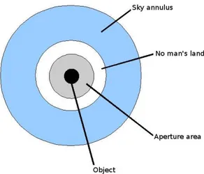
Instrumental magnitudes were then measured via aperture photometry, with an integrating radius determined by growth curves (typically about three times the average seeing) and sky subtraction performed using a 5-10 pixel wide annulus around each object (Fig. 2.1).

Hence:

mI = −2.5 log(N) (2.1)

where mI is the instrumental magnitude and N is the obtained count rate

(3)

2.1. PHOTOMETRY 33

Figure 2.1 – Schematic illustration of the aperture photometry measurement. For a few cases the aperture correction method was used to determine the object flux. Indeed, for faint objects (i.e., V >_{∼ 22) a small aperture} is needed to reduce the sky background contribution and the probability of contamination by a background source. The aperture correction also greatly helps when measuring the object flux in case of nearby stars. This method consists of measuring bright field stars with both a “small” aperture (∼ 1 FWHM) and a bigger aperture to get all the light from the sources. From the ratio of light in the small to large aperture, which is of course expressed as a magnitude difference, it is possible to determine the correction to apply to the object magnitude, measured through the “small” aperture.

In this case:

mI = −2.5 log(N) + ∆ (2.2)

where N is the count rate in the “small” aperture and ∆ is the computed aperture correction.

Atmospheric extinction is taken into account correcting the magnitudes as:

(4)

34 CHAPTER 2. DATA ACQUISITION AND REDUCTION

where m0 is the “zero airmass” magnitude (i.e., what it would be outside the

atmosphere), K(λ) is the wavelength dependent extinction coefficient and X is the airmass, defined as (in a plane-parallel atmosphere approximation):

X ∼ sec z = _{sin φ sin δ + cos φcosδ cos h}1 (2.4) where z is the zenith angle, φ is the latitude of the observatory, and δ and h are the declination and the hour angle of the observed object, respectively.

The atmospheric extinction depends by the wavelength because of several physical effects: Rayleigh scattering, ozone or H2O molecular absorption and

aerosol scattering. For example, the amount of Rayleigh scattering off of atoms and molecules, much smaller than the wavelength of light, goes as λ−4_{, so drops rapidly towards longer wavelength, while ozone has extinction}

that sharply rises blueward of about 0.32 µm, plus another small bump at about 0.6 µm. Hence, a color dependence was taken into account through a second order correction:

K(λ) = K′+ K′′_{× CI} (2.5) where K′ _{and K}′′ _{are the main (or first order) extinction coefficient and the}

color correction (or second order) extinction coefficient, respectively, and CI is a color index, defined as the difference between magnitudes in two different bands.

Finally, adding the zero point (ZP ), instrumental magnitudes were con-verted in standard system magnitudes:

M = m0 + ZP (2.6)

The above descripted calibration of the magnitudes was obtained by means of the observation of several Landolt (1992) standard fields, at different air-masses, throughout each observing night.

2.1.2 Near-infrared

At NIR wavelengths the brightness and rapid variability (∼ 5-10 minutes) of the sky requires total exposure times to be splitted in short exposures of 2-3 minutes at most (Detector Integration Time, DIT); being NDIT the number of DIT exposures averaged out within the same frame and NINT the number of frames, the total exposure time is therefore DIT × NDIT × NINT.

(5)

2.2. SPECTROSCOPY 35

Jitter imaging is used to take care of sky background issues: giving small

(i.e., no larger than a reasonably small fraction of the detector size) offsets between the different exposures, it is possible to deduce the sky background variations directly by filtering the images, and to separate the astronomical and the sky signals.

Also, unlike optical CCDs, the dark current correction is important for infrared arrays. Hence, an average of several (exposure time dependent) dark

frames have to be subtracted from subsequent images.

The data were pre-reduced (dark subtraction, flat-field correction, bad pixel cleaning, sky subtraction, recombination of the images) by using the ESO ISAAC pipeline (which runs through EsoRex, the “ESO Recipe Ex-ecution Tool”). Then, as for the visible images, target fluxes were mostly measured (with ESO-MIDAS) using classical photometry methods with aper-tures determined by the seeing and growth curves of the objects, reserving the aperture correction method to a few cases (faint target and/or nearby field stars).

To calibrate the instrumental magnitudes (using the same procedure de-scribed in the previous section for visible images), standard stars from dif-ferent catalogues (Persson et al. 1998; Hawarden et al. 2001) were observed.

2.2 Spectroscopy

2.2.1 Visible

All of the spectra were acquired through a slit oriented along the parallactic angle in order to minimize the effects of atmospheric differential refraction.

The data were reduced using ESO-MIDAS. The basic procedure for con-verting raw spectral flux measurements to reflectance spectra, as for photo-metric data, started with median bias subtraction and flat-field correction. After that, the 2-D spectra were transformed in monodimensional spectra in-tegrating the flux along the spatial axis (with aperture radius usually around 1.5 FWHM) and subtracting the sky contribution. Then, wavelength cali-bration was performed through spectral lines from different (He, Ar, Ne) calibration lamps and atmospheric extinction correction was taken into ac-count according to the extinction law for each observing site. At this point spectra were normalized usually at 0.55 µm and the reflectivity of the objects was obtained by dividing their spectra by the spectrum of a solar analog star which had been acquired close in time and airmass (to have the atmospheric conditions the most similar as possible). Finally, the spectra were smoothed with a median filter technique. This means that, using a box of about

(6)

30-36 CHAPTER 2. DATA ACQUISITION AND REDUCTION

Figure 2.2 – Illustration of the ISAACSW spec obs AutoNodOnSlit tem-plate, used in NIR spectroscopy with the ISAAC instrument at the VLT. The black dots represent the different positions of an object originally at the center of the slit. From the ISAAC user manual.

40 ˚A in the spectral direction for each point of the spectrum and a threshold around 10-15%, the original value has been replaced by the median value when this latter differed from the former by more than the threshold.

2.2.2 Near-infrared

Because of the high luminosity and variability of the sky in the NIR, the observations were carried out by moving (usually by 10 arcseconds) the object along the slit between two positions A and B (the classical nodding technique used in NIR spectroscopy). Cycles are repeated on ABBA sequences, until the total exposure time is reached. In addition to nodding, random offsets are added to the positions Ai and Bi. The random offsets, much smaller than

the “nod throw”, are generated inside a “jitter box” (Fig. 2.2). This way the sky contribution, including the random fluctuations, is effectively removed by subtracting one frame from the other.

(7)

2.2. SPECTROSCOPY 37 First steps of the reduction procedure were performed using the ISAAC pipeline: flat-fielding, wavelength calibration (through atmospheric OH lines or Xe-Ar lamp lines), A-B (or B-A) subtraction for each pair of frames (the subtracted frames hence contain positive and negative spectra), correction for spatial and spectral axes distortion, shifting and adding of the frames. The resulting combined spectrum of the object was then extracted using ESO-MIDAS. Because of the rapid changes of the absorption at NIR wavelengths, the atmospheric extinction correction cannot be done as in the visible: it is hence fundamental to get the reflectivity of the object by dividing its spectrum by that of a solar analog star observed just before or after the object, at airmass as similar as possible. As for visible data, the spectra were finally smoothed with a median filter technique (with a box of ∼ 10 ˚

(8)

(9)

Chapter 3 Rosetta asteroid targets

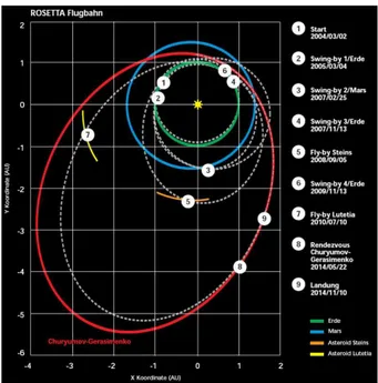
Rosetta is a space mission led by the European Space Agency (ESA) which takes its name from the Rosetta Stone, a stele of black basalt which pro-vided the key to deciphering Egyptian hieroglyphs. It was originally set to rendezvous with the comet 46P/Wirtanen in 2011, but the original launch date was postponed because of the failure of the Ariane V launcher (De-cember 2002). A new mission baseline was formed (Fig. 3.1), and Rosetta was successfully launched on March 2004 with the main objective to enter orbit around the comet 67P/Churyumov-Gerasimenko and to perform obser-vations of its nucleus and coma.

During its 10 years journey to the comet, the spacecraft performs also the fly-by of two main belt asteroids, (2867) Steins and (21) Lutetia. The fly-by with Steins took place on September 2008, while the one with Lutetia is scheduled on July 2010. An ESA Science Working Group selected these two bodies based on the results by Barucci et al. (2005c), which studied all the candidates of all the possible mission scenarios: Lutetia emerged as the most interesting target for both its large size (∼ 100 km), which makes radio science experiments feasible, and its puzzling nature with a possible prim-itive composition, which could provide insight into the early Solar System conditions; after the choice of the first target, Steins was the best candidate for a second fly-by, with its relatively unusual (E-type) spectral properties.

As already stated, the physical characterization of the asteroid targets of space missions is fundamental for both the optimization of the mission operations and the “calibration” of standard ground-based observations of asteroids (ground truth). Keeping this in mind, in the framework of my PhD I performed a ground-based investigation of asteroids (2867) Steins and (21) Lutetia, as described in sections 3.1 and 3.2 respectively.

(10)

40 CHAPTER 3. ROSETTA ASTEROID TARGETS

Figure 3.1 – Rosetta’s flight plan.

3.1 (2867) Steins

Steins is a small (few km) main belt asteroid and its ground-based investi-gation started only in early 2004, when it was included in the list of possible asteroid targets of Rosetta.

In March 2004 Steins was observed photometrically by both Warner (2004) and Hicks et al. (2004), who measured synodic periods of 6.05±0.01 hours and 6.06±0.05 hours, respectively. A full analysis of the latter set of observations was reported by Weissman et al. (2007), who obtained a revised synodic period of 6.048±0.007 hours. Imaging performed during the cruise phase of Rosetta by the Narrow Angle Camera (NAC) of the Optical Spec-troscopic and Infrared Remote Imaging System (OSIRIS), allowed K¨uppers et al. (2007) and Jorda et al. (2008) to derive Psyn=6.052±0.007 hours and

Psyn=6.054±0.003 hours, respectively. Moreover, by compiling a set of 26

visible light curves belonging to 6 data sets obtained by ground-based obser-vatories and one by the spacecraft, Lamy et al. (2008b) computed a sidereal period of 6.04681±0.00002 hours.

Visible and near-infrared spectroscopic observations of Steins obtained by Barucci et al. (2005c) revealed a spectral behavior similar to that of E-type asteroids (thought to be differentiated bodies which experienced significant heating). In particular, its spectrum resembles those of the E[II] subtype (or “Angelina-like”, from (64) Angelina) within the classification by Gaffey &

(11)

3.1. (2867) STEINS 41 Kelley (2004) and Clark et al. (2004), with the presence of a strong feature at about 0.5 µm, a weaker feature at about 0.96 µm, and a flat and feature-less behavior beyond 1 µm. These absorption features are characteristic of oldhamite, a calcium sulfide mineral which is present only in highly reduced assemblages such as aubrites (enstatite achondrite meteorites). The absorp-tion features probably arise from the presence of a trace of bivalent iron in the sulfide. Although the geochemical behavior of oldhamite in highly reduced igneous systems is not completely understood (oldhamite is an extremely un-stable element in terrestrial atmospheric conditions), it seems likely that it will be significantly enriched in early partial melts from enstatite chondrite source materials. Hence, the E[II] asteroids may be composed of basalt equiv-alents from E-chondrite-like parent bodies which underwent at least partial melting (e.g., Gaffey & Kelley 2004, and references therein). Burbine et al. (1998) proposed that the feature at 0.49 µm is due to troilite, but this is problematic because E-types are by definition very high albedo objects and troilite is naturally a very dark mineral component. It has been shown that even minute amounts of a spectrally dark component can nonlinearly darken a mineral mixture (Clark & Lucey 1984), making it very unlikely that troilite is a major component of the surfaces of these bright objects. Nevertheless, troilite is a component found in minor amounts in aubrite meteorites (Clark et al. 2004, and references therein).

Steins’ albedo was derived by Fornasier et al. (2006) on the basis of polari-metric observations carried out at ESO-VLT in 2005. Using the well-known (e.g., Cellino et al. 1999a, 2005) empirical relationship between the albedo and the slope of the polarimetric curve (polarization degree versus phase an-gle), the authors determined an albedo of 0.45±0.10, a high value consistent with the E-type classification suggested by the spectroscopic behavior. A new determination of the geometric albedo, obtained by thermal modeling of data from the Spitzer Space Telescope, inferred a value of pV=0.34±0.06

(Lamy et al. 2008a). This value appeared to be slightly low for an E-type object, although the Spitzer emissivity spectrum between 5.2 and 38 µm was consistent with that of aubrite meteorites and enstatite minerals (Barucci et al. 2008b), and confirmed the E-type classification.

3.1.1 Observational campaign

Until April 2008, neither photometric observations nor light curves of Steins were available for phase angles α < 7◦_{, while this region is particularly}

impor-tant for the determination of the asteroid absolute magnitude H and slope parameter G (see section 1.2.1).

(12)

Rosetta encounter, I participated to an observational campaign (Spring 2008) during which low phase angle visible spectroscopy and visible photometry of the asteroid were performed. These observations were important to complete the ground-based data set, and to compute the physical parameters of Steins that are fundamental for properly calibrating the imaging and spectroscopic data acquired by instruments onboard Rosetta.

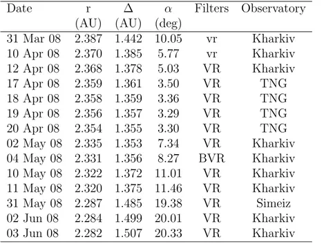
Photometric observations were carried out at the Institute of Astronomy of the Kharkiv Karazin National University (70 cm reflector), the Simeiz De-partment of the Crimean Astrophysical Observatory (1 m reflector), and the 3.6 m Telescopio Nazionale Galileo (TNG, La Palma, Spain). The observa-tional circumstances are reported in Table 3.1.

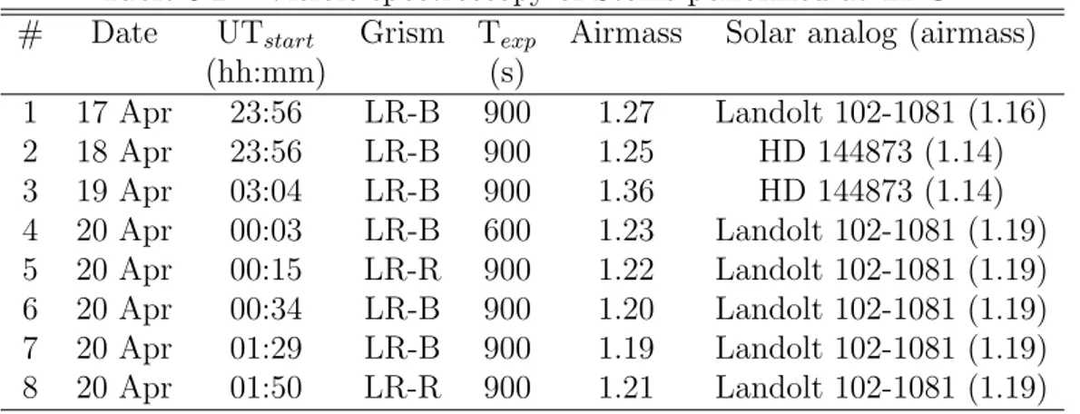
At TNG visible spectra were also acquired using the DOLORES (Device Optimized for the LOw RESolution) instrument with the low resolution blue (LR-B) and red (LR-R) grisms. Table 3.2 reports, for each spectrum, the starting time of acquisition, the used grism, the exposure length, the air-mass, and the solar analog star (with its airmass) used to obtain the Steins’ reflectivity.

Data reduction was performed as described in chapter 2 for both photom-etry and spectroscopy, and the calibrated data were corrected for light-time.

Table 3.1 – Observational circumstances for Steins (r, ∆, and α are the helio-centric distance, the topohelio-centric distance, and the phase angle, respectively).

Date r ∆ α Filters Observatory (AU) (AU) (deg)

31 Mar 08 2.387 1.442 10.05 vr Kharkiv 10 Apr 08 2.370 1.385 5.77 vr Kharkiv 12 Apr 08 2.368 1.378 5.03 VR Kharkiv 17 Apr 08 2.359 1.361 3.50 VR TNG 18 Apr 08 2.358 1.359 3.36 VR TNG 19 Apr 08 2.356 1.357 3.29 VR TNG 20 Apr 08 2.354 1.355 3.30 VR TNG 02 May 08 2.335 1.353 7.34 VR Kharkiv 04 May 08 2.331 1.356 8.27 BVR Kharkiv 10 May 08 2.322 1.372 11.01 VR Kharkiv 11 May 08 2.320 1.375 11.46 VR Kharkiv 31 May 08 2.287 1.485 19.38 VR Simeiz 02 Jun 08 2.284 1.499 20.01 VR Kharkiv 03 Jun 08 2.282 1.507 20.33 VR Kharkiv

(13)

3.1. (2867) STEINS 43 Table 3.2 – Visible spectroscopy of Steins performed at TNG.

# Date UTstart Grism Texp Airmass Solar analog (airmass)

(hh:mm) (s) 1 17 Apr 23:56 LR-B 900 1.27 Landolt 102-1081 (1.16) 2 18 Apr 23:56 LR-B 900 1.25 HD 144873 (1.14) 3 19 Apr 03:04 LR-B 900 1.36 HD 144873 (1.14) 4 20 Apr 00:03 LR-B 600 1.23 Landolt 102-1081 (1.19) 5 20 Apr 00:15 LR-R 900 1.22 Landolt 102-1081 (1.19) 6 20 Apr 00:34 LR-B 900 1.20 Landolt 102-1081 (1.19) 7 20 Apr 01:29 LR-B 900 1.19 Landolt 102-1081 (1.19) 8 20 Apr 01:50 LR-R 900 1.21 Landolt 102-1081 (1.19)

3.1.2 Light curves

Figure 3.2 shows the composite light curves derived for the V and R bands. They are consistent within the error bars and characterized by rather sym-metrical shape.

A rotational synodic period of Psyn = 6.057 ± 0.003 was computed by

applying the method developed by Harris et al. (1989a) based on Fourier analysis of light curves, as described in section 1.2.1. The light curve am-plitude is 0.20 ± 0.02 mag in both bands, which provides (from Eq. 1.10) a lower limit to the axis ratio, a/b ≥ 1.20 ± 0.02 assuming that Steins does not have considerable albedo variations and that the observed amplitude is only affected by the asteroid shape.

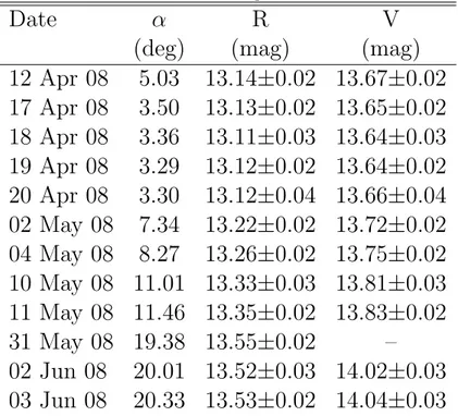
The composite light curves were used to convert all measured magnitudes into those corresponding to the light curve maximum, which is less affected by the asteroid shape. This was possible with a good accuracy, since most of the observations covered one or both maxima. Adding half of the light curve amplitude, mean R and V magnitudes for each night were derived. The obtained values are reported in Table 3.3, with a resulting color of V − R = 0.51 ± 0.03 mag.

3.1.3 Phase curve

Fig. 3.3 presents the magnitude-phase dependence of Steins in R band, where also previously published observations obtained in 2004 - 2008 by Hicks et al. (2004), Weissman et al. (2007), Jorda et al. (2008), and Lamy et al. (2008b) have been used. These measurements were corrected for the light curve am-plitude in the same way as described above. A good agreement between the data obtained at different oppositions emerges, confirming that the

(14)

ro-44 CHAPTER 3. ROSETTA ASTEROID TARGETS

Figure 3.2 – Composite R and V light curves of Steins. The coverage of the obtained spectra is shown on the top of the data. The light curve zero-point is at 0 UT on 19 April 2008. From Dotto et al. (2009).

Table 3.3 – V and R magnitudes of Steins.

Date

α

R

V

(deg)

(mag)

12 Apr 08

5.03 _{13.14±0.02 13.67±0.02}

17 Apr 08

3.50 _{13.13±0.02 13.65±0.02}

18 Apr 08

3.36 _{13.11±0.03 13.64±0.03}

19 Apr 08

3.29 _{13.12±0.02 13.64±0.02}

20 Apr 08

3.30 _{13.12±0.04 13.66±0.04}

02 May 08

7.34 _{13.22±0.02 13.72±0.02}

04 May 08

8.27 _{13.26±0.02 13.75±0.02}

10 May 08 11.01 13.33±0.03 13.81±0.03

11 May 08 11.46 13.35±0.02 13.83±0.02

31 May 08 19.38 13.55±0.02

–

02 Jun 08

_{20.01 13.52±0.03 14.02±0.03}

03 Jun 08

_{20.33 13.53±0.02 14.04±0.03}

(15)

3.1. (2867) STEINS 45

Figure 3.3 – Phase curve of Steins in the R band fitted by linear (dotted line) and H-G fit (dashed line). From Dotto et al. (2009).

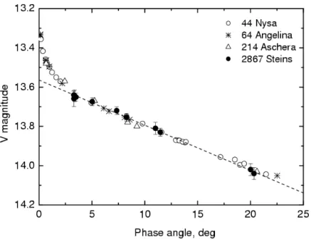
Figure 3.4 – Magnitude-phase dependence in the V band of Steins and other E-type asteroids. From Dotto et al. (2009).

(16)

tation axis of Steins is almost perpendicular to the ecliptic plane (Lamy et al. 2008b), thus that Steins is observed at almost the same aspect angle (ξ ∼ 86◦_{) in different apparitions. According to the Bowell et al. (1989)}

formalism (see section 1.2.1), all of these data were used to compute the R band absolute magnitude and slope parameter (V band phase parameters would be less accurate because of the smaller dataset), with resulting val-ues of HR = 12.86 ± 0.02 and GR = 0.42 ± 0.02. The GR here obtained

is higher than in previous works, but this discrepancy could be due to a lack of observations at phase angle lower than 7◦ _{in previously analyzed}

samples. The obtained “H-G fit” is consistent with a linear fit for the ob-served range of phase angles with slope βR = 0.026 ± 0.001 and y-intercept

R(0) = 13.04 ± 0.02 (see Fig. 3.3). The shallow slope observed for Steins is typical of E-type asteroids (e.g., Belskaya et al. 2003), and strongly supports its classification in this taxon.

A comparison of the magnitude-phase dependence of Steins and other E-types is shown in Fig. 3.4. All of these data (from Harris et al. 1989b; Belskaya et al. 2003) were obtained in the V-band and shifted in magnitude to match the Steins data. By assuming that the amplitude of the opposition effect of Steins is similar to that of the other E-type asteroids (0.23 ± 0.03, Belskaya & Shevchenko 2000), it is possible to calculate the Steins’ R absolute magnitude by adding the value of the opposition effect to R(0), obtaining a value of HR= 12.81 ± 0.03.

3.1.4 Spectral properties and modelling

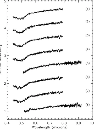
Eight spectra of Steins have been obtained during the observations at TNG (Fig. 3.5), exhibiting the typical behavior of E[II] asteroids: all of them are almost flat and featureless between 0.55 and 0.9 µm, and present the before discussed absorption signature at 0.49 µm. The spectral slopes, computed between 0.56 and 0.79 µm, are reported in Table 3.4.

The coverage of the Steins’ light curve by the eight spectra is shown in Fig. 3.2. Since the same spectral behavior is found for ∼ 30% of the rotational light curve, it is possible to argue that Steins has a quite homogeneous surface composition.

In Fig. 3.6, the spectrum #2 (LR-B grism) and the spectrum #5 (LR-R grism), which cover almost the same surface region, are plotted together. Using a radiative transfer model (based on the Hapke theory), that had al-ready been used to model the surface composition of Jupiter Trojans, Trans-Neptunian Objects, and Centaurs (e.g., Dotto et al. 2003, 2006), an attempt to reproduce the spectral behavior of Steins has been perfomed using ge-ographical mixtures of different components (i.e., distributed as different

(17)

3.1. (2867) STEINS 47

Figure 3.5 – Visible spectra of Steins normalized at 0.55 µm and shifted by 0.5 in reflectivity for clarity. From Dotto et al. (2009).

patches on the surface) selected from enstatite meteorites and correlated minerals included in the RELAB1 _{(KECK/NASA Reflectance Experiment}

Laboratory) catalog. The continuous line in Fig. 3.6 shows the synthetic spec-trum of a mixture consisting of 55% enstatite achondrite meteorite (aubrite) Mayo Belwa and 45% oldhamite (this mixture has an albedo of 0.35).

On the basis of these results the surface of Steins appears to be homo-geneous, and its composition, as already suggested by both Barucci et al. (2005c) and Fornasier et al. (2007, 2008), resembles the enstatite meteorites, in particular the aubrites, enriched in oldhamite.

1

(18)

Table 3.4 – Spectral slopes of Steins’ spectra. # Spectral slope (% / 103_˚_A) 1 _6.88±0.65 2 _7.09±0.65 3 _7.12±0.65 4 _7.48±0.65 5 _8.26±0.65 6 _7.75±0.65 7 _7.25±0.65 8 _6.48±0.65

Figure 3.6 – Spectra #2 and #5, normalized at 0.55 µm. The continuous line shows the tentative model of the Steins surface composition. From Dotto et al. (2009).

(19)

3.1. (2867) STEINS 49

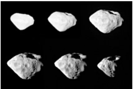
Figure 3.7 – Asteroid Steins taken by the OSIRIS instrument. The large crater at the southern (according to IAU rules, see text) pole can be seen. Images from ESA - OSIRIS Team.

3.1.5 Steins seen by Rosetta

On 5 September 2008 Rosetta successfully made a close (∼ 800 km) fly-by of Steins (Fig. 3.7). Altogether 14 instruments were switched on during the fly-by, providing spatially resolved multi-wavelength observations of the as-teroid and in-situ measurements of its dust, plasma, magnetic, and radiation environment.

Among the first obtained results, Steins resulted to be a diamond-shaped asteroid with dimensions of 4.0 × 5.9 km, dominated by a large (∼ 2 km) crater at the southern pole (Steins’s rotation is retrograde, therefore its north pole points toward the celestial south according to the rules of the Interna-tional Astronomical Union). From there a chain of 7 craters extends across the surface visible during the fly-by. More than 20 craters with diameters > 0.2 km can be counted (Keller et al. 2009). The geometric albedo resulted to be 0.40 ± 0.01 and the slope parameter G is 0.45, both typical values for E-type asteroids. The visible spectrum is slightly reddish, with a sharp drop-off in reflectance towards the near-ultraviolet region, in agreement with ground-based observations (K¨uppers et al. 2009).

The results presented in this thesis, deriving from the last ground-based dataset obtained before the Rosetta fly-by, are particularly important for the calibration and interpretation of the data acquired by the spacecraft. The analysis of the latter is still ongoing, but in general it seems that the Rosetta data are well comparable with those obtained from ground-based investigations, strengthening the ground truth.

(20)

3.2 (21) Lutetia

Although several observations of (21) Lutetia are available since a couple of decades, the nature of this asteroid is still controversial. Its rotational period was firstly measured by Zappala et al. (1984), who found P = 8.17 ± 0.01 hours, and later refined by Torppa et al. (2003), who found P = 8.165455 hours and also computed the pole coordinates obtaining a model with axis ratios a/b = 1.2 and b/c = 1.2. IRAS (InfraRed Astronomical Satellite) ob-servations of Lutetia gave a diameter of about 96 km and an albedo of 0.22. Because of the latter high value, later confirmed by Mueller et al. (2006) who found a value of 0.208 ± 0.025, Lutetia was classified as a M-type asteroid by Barucci et al. (1987) and Tholen (1989). Considering that M-types have spectral properties and albedo values consistent with Fe-Ni metal and are generally thought to be the metallic cores of differentiated asteroids exposed after catastrophic disruptions, Lutetia was supposed to be an evolved object which suffered a strong heating and alteration. Nevertheless, further obser-vations did not confirm the metallic nature of Lutetia, suggesting rather a primitive surface composition. Howell et al. (1994) and Burbine & Binzel (2002) showed that the infrared spectrum of Lutetia is unusually flat com-pared to other M-type asteroids. Moreover, observations obtained by Barucci et al. (2005c) and Birlan et al. (2004) suggested a similarity with carbona-ceous chondrite spectra which characterize the C-type asteroids. Lazzarin et al. (2004) obtained several visible spectra showing variations with the ro-tational phase, and the possible presence of features at 0.43 and 0.51 µm probably associated to hydrated silicates. In a single spectrum the authors also found two minor absorptions at ∼ 0.6 µm and 0.80-0.85 µm, which have been already detected in the spectra of aqueously altered meteorites and several hydrated asteroid classes. Lazzarin et al. (2009) presented a wide mineralogical assessment of Lutetia, found broad complex features be-tween 0.45 and 0.55 µm, and two narrower features around 0.47 and 0.52 µm. Some more, the polarimetric properties of Lutetia are better explained by a carbonaceous chondritic composition than by metallic composition (Bel-skaya & Lagerkvist 1996), its radar albedo would be the lowest measured for any M-class MBA (Magri et al. 1999), and recent ground-based infrared observations allowed Carvano et al. (2008) to obtain a geometric albedo of 0.129, significantly lower than all the previous estimations. The latter au-thors explained the wide range of computed albedo values as the evidence of inhomogeneities on the surface of Lutetia, suggesting the presence of one or more large craters on the northern hemisphere.

Rivkin et al. (2000) detected an absorption feature at 3 µm, diagnostic of water of hydratation and further evidence that Lutetia is largely

(21)

non-3.2. (21) LUTETIA 51 metallic. Birlan et al. (2006) confirmed the presence of the 3 µm band and defined an upper limit of 0.5% concerning a possible absorption band at about 3.1 µm. Spitzer observations carried out by Barucci et al. (2008b) between 5.2 and 38 µm revealed a clear analogy to carbonaceous chondrite meteorites, in particular the CO-CV types.

More recently, Vernazza et al. (2009) obtained spectra of Lutetia which seem to indicate that the surface composition of this object could have some genetic link with more evolved enstatite chondrite meteorites.

Hence, even if most of the authors agree about the primitive composition of Lutetia, on the basis of the observational evidence this asteroid appears to be an atypical puzzling object, whose nature is still far to be fully understood.

3.2.1 Observations

In order to enhance the view of Lutetia prior to the Rosetta fly-by, I con-tributed to a spectroscopic investigation of this intriguing object. Obser-vations have been carried out in November 2008 at the TNG, using the DOLORES instrument with the low resolution blue (LR-B) grism. Table 3.5 reports, for each obtained spectrum, the starting time of acquisition, the ex-posure length, the airmass, and the airmass of the spectrum of solar analog Hyades 64 used to obtain the Lutetia’s reflectivity.

Data reduction followed the procedures described in chapter 2 (acquisition times were corrected for light-time). The resulting spectra are cut at 0.45 µm, since at lower wavelengths their behavior is strongly affected by the spectra of the solar analogs.

3.2.2 Results and discussion

The obtained spectra are shown in Fig. 3.8. Table 3.6 reports the coverage of the rotational phase and the spectral slope (computed between 0.6 and 0.75 µm) for each of them.

The general spectral behaviour is similar in all the spectra, but some dif-ferences are evident. All of them exhibit two spectral features at about 0.47-0.48 µm and around 0.6 µm. Both these spectral features have been already seen on the spectra of (21) Lutetia (see above). The signature at ∼ 0.47-0.48 µm was already detected on spectra of Lutetia by Lazzarin et al. (2009), who interpreted them as due to spin-allowed crystal field transitions in Ti3+

in pyroxene Y sites (pyroxenes have the general formula XY(Si,Al)2O6),

al-though Hazen et al. (1978) suggested that in lunar pyroxenes such a band could be due to the superimposition of Ti3+ _{and Fe}2+ _effects.

(22)

Table 3.5 – Visible spectroscopy of Lutetia performed at TNG. # Date UTstart Texp Lutetia airm. Hyades 64 airm.

(hh:mm) (s) 1 27 Nov 23:39 8 1.07 1.04 2 27 Nov 23:53 30 1.05 1.04 3 28 Nov 00:49 40 1.01 1.04 4 28 Nov 01:33 40 1.02 1.04 5 28 Nov 02:23 40 1.07 1.04 6 28 Nov 03:05 40 1.14 1.04 7 28 Nov 03:54 40 1.30 1.04 8 28 Nov 04:32 40 1.50 1.04 9 29 Nov 22:18 40 1.23 1.02 10 29 Nov 23:12 40 1.09 1.02 11 29 Nov 23:13 30 1.09 1.02 12 30 Nov 00:07 30 1.03 1.02 13 30 Nov 00:57 40 1.01 1.02

Table 3.6 – Coverage of the rotational phase and slope of each obtained spectrum of Lutetia.

# Rotational phase Spectral slope

(% / 10

3

_˚

_A)

1

0.018 _1.5±0.5

2

0.046 _1.0±0.5

3

0.161 _1.4±0.5

4

0.251 _1.8±0.5

5

0.353 _2.2±0.5

6

0.438 _2.0±0.5

7

0.538 _2.1±0.5

8

0.616 _1.7±0.5

9

0.731 _0.7±0.5

10

0.841 _1.4±0.5

11

0.843 _1.6±0.5

12

0.953 _1.7±0.5

13

0.056 _1.7±0.5

(23)

3.2. (21) LUTETIA 53

Figure 3.8 – Visible spectra of Lutetia normalized at 0.55 µm and shifted of 0.1 in reflectivity for clarity. From Perna et al. (2010b).

(24)

The band at ∼ 0.6 µm was seen in one of the spectra published by Laz-zarin et al. (2004) and it is generally attributed to charge transfer transitions in minerals produced by aqueous alteration of anhydrous silicates (Vilas et al. 1994), but can be also present on pyroxenes (e.g., Burns et al. 1976). The depth of the spectral features, relative to the continuum reflectance, is of about 1% in all the spectra, not exhibiting any evident variation. Con-versely, as reported in Table 3.6 and shown in Fig. 3.9, the spectral slopes computed between 0.6 and 0.75 µm exhibit a periodic variation (in partic-ular, a clear inhomogeneity emerges in correspondence with the spectrum # 9). This variation of the spectral slope of Lutetia through the rotational phase, can be interpreted as due to the presence of inhomogeneities on the observed portion of the asteroid surface. These inhomogeneities could be re-lated to the chemical/mineralogical composition, as well as to the structure of the surface as the possible result of the presence of craters on the surface of Lutetia.

Considering the pole solution (λ = 39◦_{, β = 3}◦_{) found by Torppa et al.}

(2003) and the cartesian coordinates vector of Lutetia with respect to the TNG site (retrieved from the JPL/HORIZONS system2_{), the aspect angle}

(Fig. 3.10) during the observations was measured as:

ξ = arccos(|~V | • | ~C|) (3.1) where |~V | is the unit vector of the pole of Lutetia, | ~C| is the unit vector of its cartesian position, and the symbol • indicates the dot product operation. All the spectra were obtained at an aspect angle ξ ∼ 30◦_{, and are therefore}

referred to the same asteroid emisphere. On the basis of these results, it is possible to support the hypothesis formuled by Carvano et al. (2008) that one or more craters/inhomogeneities can be present on the surface of Lutetia (as shown in Fig. 3.9, these inhomogeneities could cover up to 20% of the surface of Lutetia).

These data are useful in the assessment of the physical nature of Lutetia, and will constitute a fundamental start up for the calibration, analysis and interpretation of the data acquired by the instruments onboard the Rosetta spacecraft.

2

(25)

3.2. (21) LUTETIA 55

Figure 3.9 – Spectral slope vs. rotational phase of Lutetia, computed consid-ering a rotational period of 8.165455 hours (Torppa et al. 2003). From Perna et al. (2010b).

Figure 3.10 – Schematic illustration of viewing geometry for a Solar System body.

(26)