Chapter 4
Active Yaw Control
4.1
ESP
As already mentioned in the introduction, nowadays many cars are provided with stability control systems. Now we describe when and how these kind of devices act, focusing on the ESP and on our innovative system.
4.1.1
ESP Working Principles
The ESP is an Active Yaw Control studied in order to increase vehicle safety, avoiding excessive oversteering or understeering behavior. This system receives information from several sensors installed on the vehicle (steering wheel angle, yaw-rate, yaw-acceleration, wheel speeds, etc.), and through these signals a software is able to estimate instant by instant the car motion. Comparing the “real” estimated motion with an ideal behavior provided by software it is possible to understand if the car is behaving in a stable, foresee-able and controllforesee-able way, or if the driver is probably loosing control.
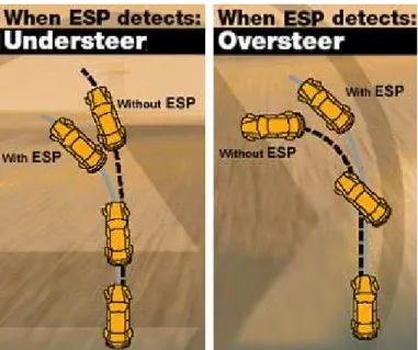
Considering for example a left-hand curve, if an excessive oversteer is detected the system activates the front-right brake, such a way to create a negative longitudinal force (Fx12),
and in the same time to decrease the lateral force (Fy21). Both these effects contribute to
decrease the yaw-acceleration (2.3), such a way to avoid that the car begins to spin around or anyhow to prevent an undesired behavior that, if not controlled by a professional driver, can be dangerous (fig.4.1).
By a similar principle if an excessive understeer was detected the ESP would activate the rear-left brake, to generate a pro-cornering yaw moment (fig.4.1).
Figure 4.1: Effects of the ESP on vehicle motion
4.1.2
ESP Simulink Model
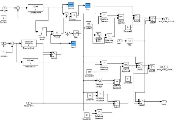
In our model we designed an ESP which is represented in fig.4.2. Our ESP receives as inputs: the instantaneous yaw rate, a reference yaw rate, the vehicle lateral acceleration, an estimated lateral acceleration, the front and rear drive torques, and the steer angle. Now we illustrate how these signals are obtained and afterwards we describe how our ESP processes them to recognize a dangerous situation.
4.1.3
“Reference Yaw Rate” Value
The “Reference Yaw Rate” value is one of the inputs used to decide whether to activate or not to activate the ESP. This input is worked out by the following expression
YR=
r− rref
|rref|
sign(r) (4.1)
The yaw rate (r) is a quantity that can be measured by a sensor, and rref is the reference
yaw rate.
To calculate the reference yaw rate our ESP needs, we built a “sub-model” of car. This is a “Single Track Model” ( [6], [11]) provided with linear tyres. In this case we are allowed to use this model because it is not affected by the ESP intervention1
. The
1Actually the brake action influences the wheel speeds then ,as explained further on, the estimated ve-hicle longitudinal speed. However we can neglect this phenomenon since it proved not to have a substantial effect.
Figure 4.2: ESP subsystem
internal “sub-system” in fact just provides the reference motion we want the “real” car to follow (if necessary by means of the Active Yaw Control), but we do not apply to this any brake torque. In addition the ideal motion is surely characterized by a longitudinal speed much higher than both the side velocity and the speeds produced by the yaw rate. These conditions assure that the “Single Track Model” represents correctly the “reference vehicle” behavior.
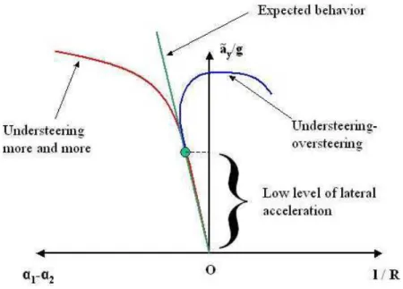
We modelled linear tyres because a non professional driver, if for example a car is understeering when the lateral acceleration is low (situation which occurs when the tyres are working in their linear zone), probably he expects a similar understeering behavior also when the lateral acceleration increases. It means that the driver is prepared for the motion that the vehicle would have if the whole tyre characteristic was linear. For these reasons he could be annoyed by a vehicle with highly non linear behavior, or for example he could be not able to control the car that suddenly becomes oversteering if the lateral acceleration exceeds a threshold value (fig.4.3). Our “sub-model” calculates the yaw-rate which the
Figure 4.3: Expected vehicle behavior in comparison with two possible real handling dia-grams
“reference car” would be going to reach in steady state conditions by the relation [6] rss= rref =
C1C2lu
C1C2l2 − mu2(C1a− C2b)
δ (4.2)
C1,2 are the cornering stiffnesses of the front and the rear axle. Whereas a linear tyre
is representative of low lateral forces, hence low lateral acceleration conditions, we are allowed not to take into account the lateral load transfer to estimate C1,2. To evaluate
them we calculate BCDy1,2 considering the static vertical load, then using the following
relation C1,2 = 2BCDy1,2, as explained in [6].
However we have to consider that the longitudinal speed is not a value provided by sensors on a real car, therefore to work out rref we had to find out a way to approximate it.
We observed that to estimate u we could measure just the wheel speeds, and to use the subsequent formula
uest=
re(ω11+ ω12+ ω21+ ω22)
4 (4.3)
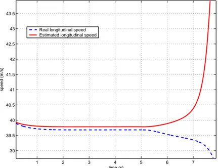
For example in fig.4.4 the real speed and the estimated speed are compared during a manoeuver that makes the car spin around because a wheel suddenly looses grip (after 5
s). We can notice that the speed value computed by (4.3) is rather similar to the real value during the first 7 seconds, during which β2
is quite little (indicatively smaller than 10 deg). Considering that to keep stability an ESP system must start acting within few instants after the loss of grip it is easy to understand that our estimated value can be an acceptable approximation of the longitudinal speed in order to detect a dangerous condition in time.
1 2 3 4 5 6 7 39 39.5 40 40.5 41 41.5 42 42.5 43 43.5 time (s) speed (m/s)
Real longitudinal speed Estimated longitudinal speed
Figure 4.4: Comparison between the real longitudinal speed and the estimated longitudinal speed
To estimate u some problems arise in case the ESP acts for a long time, but without succeeding in holding β in a small range. Further on we illustrate how we solved these problems.
Obviously we want to keep “YR” as close to zero as possible, in fact “YR” −→ 0 =⇒
r−→ rref. It means also to try to keep the estimated instantaneous “R” distance, defined
as the distance between the vehicle instantaneous center of velocity and the longitudinal symmetry axis of the car (fig.4.5), close to the “R” distance of the ideal trajectory. In fact, as mentioned in [6] we can obtain the simple kinematic relation R = u
r and, considering
u≈ uest, if r = rref also R ≈ Rest= Rref.
Unfortunately we found out that an ESP strategy based only on the “YR” value could
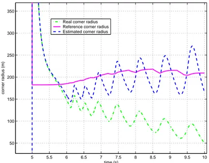
fail in particular cases, usually in oversteering conditions. In fact some simulations provided results like those shown in fig.4.6.
2β is the body slip angle, defined as β = arctanv
Figure 4.5: Definition of “R” distance
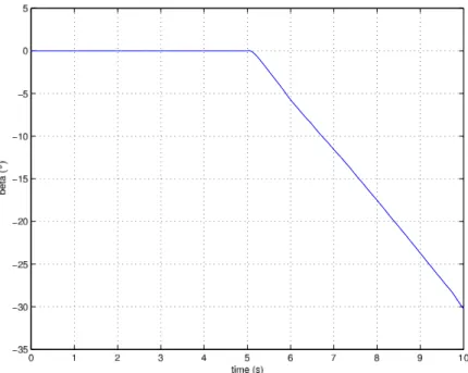
The estimated curve radius remains quite close to the reference radius during the whole simulation, but the real radius deviates from the reference input. We also noticed that this behavior matched with a β angle decreasing more and more (fig.4.7), and when the |β| angle was quite wide the uest began to overestimate u too much, in such a way that the
estimated car behavior differed notably from the real behavior. Clearly this fact causes an ESP action that is insufficient, and for this reason we needed to improve our system
5 5.5 6 6.5 7 7.5 8 8.5 9 9.5 10 50 100 150 200 250 300 350 time (s) corner radius (m)
Real corner radius Reference corner radius Estimated corner radius
Figure 4.6: Real, estimated and reference “R” distance in case of inefficacious ESP inter-vention
Figure 4.7: Body slip angle in case of inefficacious ESP intervention adding another parameter to control.
4.1.4
“Lateral Acceleration” Difference
The second parameter we decided to keep under control was the “AL” (Lateral
Accelera-tion) difference, defined as
AL = (˜ay − ay) sign(r) = (uestr− ( ˙v + ur)) sign(r) (4.4)
In steady state conditions ˙v is equal to zero, or in any case also during a transitory, apart from the first instants after a steering action, ˙v can be usually considered negligible with respect to ur. Thus to hold AL close to zero means to keep uest close to u. In this way
we managed to hold β within a small range. We also want to point out the fact that, neglecting ˙v, a dangerous oversteer matches with an AL > 0 but even if an oversteering
manoeuver is very violent, and ˙v cannot be ignored for example it is negative (considering a left-hand curve) and it contributes to increase AL without interfering negatively on the
ESP control strategy (we deal with the ESP strategy in the next paragraph). Moreover we found out that to control only AL could be sufficient to prevent oversteer, but we kept
4.1.5
ESP Strategy
The brake torque to apply to dominate the vehicle motion is provided by a PI controller which arranges it to keep the two inputs (YR and AL) close to zero, as schematically
illustrated in fig.4.8. If the controller output is positive (situation corresponding to a detected understeer) the brake torque is applied to a rear wheel, if it is negative (oversteer) it is applied to a front wheel (clearly with positive sign). We select to activate the left or right brake depending on “sign(r)”. For example, referring to the front axle, we brake the left wheel if r is positive, and we brake the right wheel if r is negative. The opposite occurs with regard to the rear axle.
eYR = YR,ref− YR eAL = AL,ref− AL Mb(t) = PYReYR+ IYR Z t 0 eYRdt | {z } P IYR + PALeAL+ IAL Z t 0 eALdt | {z } P IAL (4.5)
However a normal PI controller is not suitable to represent an ESP since the ESP acts only when a really dangerous condition arises, but the PI provides an output generally different from zero every instant, that is to say it would activate the brake system con-tinuously. Then, in order to make our system more realistic, we decided to activate the brake system only in case the output provided by the controller had exceeded an upper threshold, or a lower threshold. More exactly we do not activate a brake as soon as the controller output is bigger (or smaller) than a threshold but we check that the output exceeds the limit also some hundredths of second later, before deciding to act. We created this loop in order to avoid to activate a brake when the situation does not really require an ESP intervention but somehow the PI inputs present a peak, for example because the steer angle suddenly passes from zero to a different value, hence the PI output is great. Furthermore, in some critical manoeuvres, for example if in a rear-wheel drive car the steer angle is very wide (obviously it depends on the speed), it can occur that the two inputs would need opposite outputs to be brought closer to zero. This fact causes a system response which is unsatisfactory for both YR and AL. We decided that the most important
between the two inputs is AL. We prefer to obtain a β angle quite little, even if the car
takes the bend wider than the “reference curve”, rather than to have a car which follows a trajectory closer to the reference, but with an excessive body slip angle. This kind of motion in fact makes the driver perceive the situation as dangerous. In addition, as men-tioned above, to consider only YR can cause a car which actually drives along a trajectory
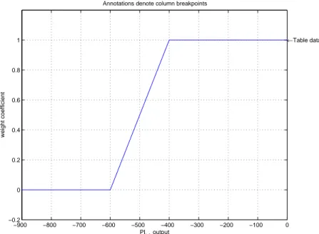
very different from the estimated trajectory, such a way to make inefficacious the Active Yaw Control. To avoid that the controller behaves in this wrong way we multiply the output of the PIYR controller by a coefficient between 1 and 0, which starts decreasing if
PIAL exceeds a lower threshold, following a curve like that shown in fig.4.9.
We want to point out the fact that until now we did not limit the maximum brake torque the ESP system can apply, and it is unrealistic (the ESP systems in production do not exploit the maximum longitudinal force a tyre can transfer) and it is dangerous because if the applied brake torque is excessive it causes the wheel lock. For these reasons we want to determine the maximum acceptable brake torque. Therefore the lateral load transfer is estimated using a simple linear relation (mentioned in [6]).
∆Fz1 = b ld1+ kφ1 kφ(h − d) t Y (4.6)
−900 −800 −700 −600 −500 −400 −300 −200 −100 0 −0.2 0 0.2 0.4 0.6 0.8 1 ←Table data PILA output weight coefficient
Annotations denote column breakpoints
Figure 4.9: Weight coefficient the PIYR output is multiplied by
∆Fz2= a ld2+ kφ2 kφ(h − d) t Y (4.7)
The total side force (Y ) is calculated multiplying the lateral acceleration ay (measured
through sensors) by the vehicle mass (m). Then, we have all the elements to calculate an approximation of Dx (2.23) (it is the peak force in pure longitudinal slip conditions) and
we multiply this value by the distance between the ground and the slip wheel axis (H) and by a safety factor (in general close to 0.5). This is the maximum brake torque applicable at a non driven wheel. Obviously an eventual drive torque affects the forces a tyre transfers to the street. To consider this fact we sum the drive torque applied to the wheel we want to brake to the brake torque previously calculated. In this way we obtain the maximum brake torque we really wish to apply. Clearly on our car we need a model of “Haldex” coupling to take into account the effects of the redistribution of torque, to estimate the drive torque.
Moreover, in order to build an ESP model as realistic as possible we created a system that checks the controller output ten times per second (in fact a real system does not receive signals from sensors continuously, and the CPU needs time to process the inputs), and it keeps the output constant during the time between two subsequent checks (obviously it may be zero).
In the end, in order to have a more realistic performance with reference to the brake torque, and to limit unrealistic peaks, for example in the vehicle speeds, due to the fact that the software calculates a numerical solution of the equations and it is negatively affected by discontinuities in the inputs, we do not use in the balance equation (2.4) the brake torque calculated as mentioned above, but we filter it by means of a simple first order filter, which equation is
Kd˜x
dt + ˜x= x (4.8)