Stage 0: Initial setup

1 Scope: This is a preliminary step to create the root folder that will contain the

sub-folders of the different calculations. In addition, all the variables assigned to relevant

information (e.g., input/output files names, folder names, number of states, torsional

angle of photo-isomerization) are storage as a dictionary in a pickle_features_rlx_scan

file, in pickle format. This file serves for parsing the stored variables as arguments to

the different routines of the module, and it is updated each time that a new variable

is defined. Indeed, it is the only argument that routines R1.RS-R4.RS receive/return

to then unpack the specific variables needed to operate.

1 Routine R0.RS: step_initial_setup_rs()

1 Root folder: <<Relaxed_Scan_n-roots_project_name>>

Stage 1: Identification of the chromophore configuration and selection of

the photo-isomerization coordinate

1 Scope: In this step, the configuration of the retinal chromophore at the S

min

structure is automatically identified (i.e., all-trans, 13-cis, 11-cis, 9-cis) by using the

low-level function arm_get_ret_configuration(). Based on such information, the

photo-isomerization coordinate (e.g., C

-C

=C

-C

for all-trans and 13-cis

config-urations) is defined, and the corresponding dihedral angles to be constrained during

the geometry optimizations are characterized (

∠

[a,b,c]).

Then, the input geometry for the first point of the RS is setup by using the

low-level function arm_get_ret_dihedrals() to get the relevant dihedrals of the S

min

structure (

∠

[a,b,c]).

1 Routine R1.RS: step_arm_initial_casscf_opt_rs(pickle_features_rlx_scan)

1 Working folder: <<initial_setup_rlx_scan_n-roots_project_name>>

1 Scope: This step consists on the computation of the relaxed scan (RS) by performing

a series of subsequent constrained optimizations, to explore the photo-isomerization

characteristic of the given r PSB. The RS is computed for the change in torsional angle

from the S

min structure to a value of |90| degrees. The magnitude and sign of the

main torsional dihedral that defines the photo-isomerization coordinate (i.e.,

∠

[a]),

is used to determine if the chromophore follows a clockwise or counter-clockwise motion

during the photo-isomerization. This information is crucial to decide if the magnitude

of

∠

[a] should be either increased or decreased in a given step_size. In this

regard, the following criteria is employed to define each of the successive points:

∠

[x{a, b, c}] =



























∠

constr

[x] + step_size,

if 90 >

∠

[x] > 0

∠

constr

[x] + step_size,

if − 90 >

∠

[x] < 0

∠

constr

[x] − step_size,

if 90 <

∠

[x] > 0

∠

constr

[x] − step_size,

if − 90 <

∠

[x] < 0

(A.2.1)

Once the new torsional angle is defined, a constrained geometry optimization is

per-formed at the n-roots SAn-CASSCF(12,12)/AMBER/6-31G(d) level, following the

gradient of the S

state. (see Section A.2.2.1). Each time that one geometry

opti-mization finishes, the convergence of such a calculation is evaluated. If it converges,

its output files are used as an input for the next constrained geometry optimization.

1 High-level function:

arm_casscf_scan_point -xyz [A

∠

] -key [B1] -jobiph [C

∠

] -espf

[D

∠

] -nr n -const

∠

[a,b,c] -o project_name

1 Routine R2.RS: step_arm_casscf_scan_point(pickle_features_rlx_scan)

1 [Open]Molcas/Tinker template:

constrained_casscf_opt.j2 {{n_roots}} = n,

{{rlxroot}}= 2

1 Working folder: <<casscf_scan_point_n-roots_project_name>>

1 input/outputs: <project_name_casscf_scan_point_n-roots_angle.*>

1 Communicator file: <project_name_casscf_scan_point_n-roots_angle.finished>

[-] Module: a_arm_rs

[-] Pickle file: project_name_RS_n-roots.pickle

1 Scope: The energy of the each of the N structures produced during the RS in R2.RS

is re-evaluated via single point m-roots single-state CASPT2(12,12)/6-31G(d)

calcu-lation.

1 High-level function: arm_caspt2_sp -xyz [AN] -key [B2] -jobiph [CN] -mr

m -o project_name

1 Routine R3.1.RS: step_arm_caspt2_sp_rs(pickle_features_rlx_scan)

1 [Open]Molcas/Tinker template: sp_caspt2.j2

{{m_roots}} = m

1 Working folder: <<sp_caspt2_n-roots_project_name_N_RS>>

1 input/outputs: <project_name_N_RS_sp_caspt2_m-roots.*>

1 Communicator file: <project_name_sp_caspt2_RS_m-roots_N.finished>

[-] Module: a_arm_rs

[-] Pickle file: project_name_RS_n-roots.pickle

[-] Current stage of the module: step_arm_caspt2_sp_rs

This file is not required for the execution of successive routines.

Stage 3.2: Energy evaluation of the RET in vacuum at the n-roots CASPT2

level for each of the structures of the RS

1 Scope: The energy of the retinal chromophore (RET) in vacuum, extracted from

each of the N structures produced during the RS, is evaluated via single point

m-roots single-state CASPT2(12,12)/6-31G(d) calculation.

1 High-level function: arm_caspt2_sp_ret -xyz [EN] -mr m -o project_name

1 Routine R3.2.RS: step_arm_caspt2_sp_ret_vacuum_rs(pickle_features_rlx_scan)

1 [Open]Molcas/Tinker template: sp_caspt2_ret51.j2

1 Working folder: <<sp_caspt2_ret51_n-roots_project_name_N_RS>>

1 input/outputs: <project_name_sp_caspt2_ret51_RS_m-roots_N.*>

1 Communicator file: <project_name_sp_caspt2_ret51_RS_m-roots_N.finished>

[-] Module: a_arm_rs

[-] Pickle file: project_name_RS_n-roots.pickle

a‑ARM: Automatic Rhodopsin Modeling with Chromophore Cavity

Generation, Ionization State Selection, and External Counterion

Placement

Laura Pedraza-González,

Luca De Vico,

Marı ́a del Carmen Marı ́n,

Francesca Fanelli,

and Massimo Olivucci

*

†_{Department of Biotechnologies, Chemistry and Pharmacy, Università degli Studi di Siena, via A. Moro 2, I-53100 Siena, Italy} ‡_{Department of Life Sciences, Center for Neuroscience and Neurotechnology, Università degli Studi di Modena e Reggio Emilia,}

I-41125 Modena, Italy

¶_{Department of Chemistry, Bowling Green State University, Bowling Green, Ohio 43403, United States}

*

ABSTRACT: The Automatic Rhodopsin Modeling (ARM) protocol has recently been proposed as a tool for the fast and parallel generation of basic hybrid quantum mechanics/ molecular mechanics (QM/MM) models of wild type and mutant rhodopsins. However, in its present version, input preparation requires a few hours long user’s manipulation of the template protein structure, which also impairs the reproducibility of the generated models. This limitation, which makes model building semiautomatic rather than fully automatic, comprises four tasks: definition of the retinal

chromophore cavity, assignment of protonation states of the ionizable residues, neutralization of the protein with external counterions, andfinally congruous generation of single or multiple mutations. In this work, we show that the automation of the original ARM protocol can be extended to a level suitable for performing the above tasks without user’s manipulation and with an input preparation time of minutes. The new protocol, called a-ARM, delivers fully reproducible (i.e., user independent) rhodopsin QM/MM models as well as an improved model quality. More specifically, we show that the trend in vertical excitation energies observed for a set of 25 wild type and 14 mutant rhodopsins is predicted by the new protocol better than when using the original. Such an agreement is reflected by an estimated (relative to the probed set) trend deviation of 0.7 ± 0.5 kcal mol−1(0.03± 0.02 eV) and mean absolute error of 1.0 kcal mol−1(0.04 eV).

1. INTRODUCTION

Vertebrate, invertebrate, and microbial rhodopsins constitute an ecologically widespread class of membrane photoresponsive proteins driving fundamental biological functions such as vision, photoentrainment, chromatic adaptation, gating, and ion-pumping.1−3 The recent discovery of a new family of light-sensing microbial rhodopsins4−7indicates that we do not still fully comprehend the vast distribution and functional diversity of these systems, which are likely to exploit, globally, an amount of sun-light energy larger than that harnessed by photosynthetic systems.

In spite of their functional diversity, rhodopsins display a remarkably common protein architecture featuring seven α-helices forming a cavity hosting a retinal protonated Schiff base (rPSB) chromophore covalently bound to a lysine located in the middle of helix VII (helix G for microbial rhodopsins).2 Furthermore, the protein functions are invariably initiated by the photoisomerization of the chromophore triggered by the absorption of light of a specific wavelength.8−12

The molecular-level understanding of how variations in the amino acid sequence can modify the functionality of the rhodopsin

molecular architecture appears to be not only central to photobiology13−20but of importance for the rational design of synthetic mimics21−23and artificial molecular devices.24−26

In the past, the investigation of how rhodopsin sequence variations modify the residue−chromophore interaction, and in turn, the protein light-response has been limited to a relatively, small number of cases.27−32For instance, the comprehension of how such variation determines a change in the wavelength of absorption maximum (λmaxa ) in tens of rhodopsins or rhodopsin

mutants, was studied as thefirst stage in the understanding of functional variation.20 However, it is apparent that a solid comprehension of how different functions emerged would require the comparative investigation of entire arrays of rhodopsins, thus actively searching for common molecular-level (e.g., residue type, placement, and conformation) traits associated with an observed property.

There is another reason for moving from the investigation of few rhodopsins to the investigation of larger rhodopsin arrays.

Received: January 23, 2019 Published: March 27, 2019

Article

pubs.acs.org/JCTC Cite This:J. Chem. Theory Comput. 2019, 15, 3134−3152

© 2019 American Chemical Society 3134 DOI:10.1021/acs.jctc.9b00061 J. Chem. Theory Comput. 2019, 15, 3134−3152

Downloaded via UNIV DEGLI STUDI DI SIENA on November 12, 2020 at 11:25:46 (UTC).

Rhodopsins are of central importance in the field of optogenetics.3,11,33−37 In optogenetics, specific microbial rhodopsins and/or their mutants are expressed in neurons, with the aim of activating, inhibiting, or visualizing neuronal activity through their interaction with light of a specific wavelength. In this context, the search for novel or better optogenetics tools (e.g., rhodopsins with specific λmaxa values)

requires the construction and screening of several sets of mutants of one or more rhodopsins.3,11,37−40_{Indeed, red-shifted} mutants, which minimize light scattering and absorption by biological tissues, are presently a target of great impor-tance.39,41−46As discussed above, both the understanding of function variability and the search for mutants with desired properties call for a comparative investigation of large arrays (e.g., hundreds, if not thousands) of rhodopsins with different amino acid sequences. In principle, this type of investigation could be carried out experimentally via expression and purification of rhodopsins from many organisms or, in the case of mutant screening, using directed evolution methods based on random mutagenesis. However, this appears to be an expensive and unpractical research effort to be carried out systematically. As we will now discuss, these issues can, in principle, be pursued through computational means, provided that novel and specialized protocols become available.

Arguably, a computational protocol suitable for the investigation of large arrays of photoresponsive proteins must be based on the construction of hybrid quantum mechanical/ molecular mechanical (QM/MM) models.47−51_{In fact, QM/} MM models decrease the computational cost by limiting the size of the protein moiety treated at the expensive QM level. For instance, in the rhodopsin models considered here, the rPSB chromophore is treated at the QM level using a multicon figura-tional quantum chemical method, whereas the protein itself is treated at the inexpensive MM level using a suitable forcefield. However, even though the application of such technology had, and still has, an important impact for rhodopsin studies, conventional QM/MM models are, almost regularly, computa-tionally complex models which are built manually and feature different QM methods and MM force fields when designed by different research groups. For this reason, they are often (i) time-consuming to construct, (ii) noncongruous (e.g., not com-parable), and (iii) error prone. Features i−iii impair the production of such models for extended rhodopsin arrays.

The recently proposed Automatic Rhodopsin Modeling protocol (from now on called ARM)52represents afirst attempt toward the automated and fast generation of congruous QM/ MM models of rhodopsins. As illustrated inFigure 1, ARM models are specialized QM/MM models and, in general, would not be applicable to other (e.g., cytoplasmic) photoresponsive proteins. ARM is not designed to produce the most accurate QM/MM models possible (see, for instance, the models of refs

50and53targeting accurate spectroscopic studies), but basic, gas-phase, and computationally fast models aimed at the rationalization and prediction of trends between sequence variability and function. Therefore, ARM aims to satisfy the following desirable features suitable for the generation of arrays of models: automation, so as to reduce building errors and avoid biased QM/MM modeling; speed, so as to deal with large sets of rhodopsins and/or rhodopsin mutants; documented accuracy, so as to be able to translate results into an experimentally assessable hypothesis; transferability, so as to treat rhodopsins with large differences in sequence (i.e., organism belonging to different life domains and kingdoms).

The current version of ARM has been tested for the prediction of trends inλmaxa of a limited set of wild type and mutant

vertebrate, invertebrate, and microbial rhodopsins,10,20,52,54,55 showing good agreement with experimental data. The required input includes (A) an X-ray crystallographic structure or comparative model of the protein in PDB (Protein Data Bank) format,56,57 (B) a list of residues forming the chromophore cavity, (C) the protonation states of ionizable side chains, and (D) the position of extracellular (OS) and intracellular (IS) counterions. As we will detail below, the main drawback of ARM is that it is, substantially, only a semiautomatic (i.e., not fully automated) protocol, as the generation of its input is achieved through a manual manipulation of the template structure necessary to provide the information on points A−D.52 Furthermore, due to possible different user choices (e.g., during the placement of IS and OS counterions), the reproducibility of the results cannot be guaranteed. The latter is a worrisome aspect, since the produced ARM model and, consequently, the calculated properties may be user-dependent. Such limitations, added to the human error factor, represent a serious issue when the target is the generation of hundreds of rhodopsin models (see for instance ref58for an example where this would be the case).

In order to overcome the above-described limitations, here we report a novel version of ARM named a-ARM. We will show that, when adopting certain default choices/parameters, a-ARM is capable of performing automatically (i.e., avoiding user manipulation) the following four key steps: (A) definition of the chromophore cavity, (B) assignment of protonation states of

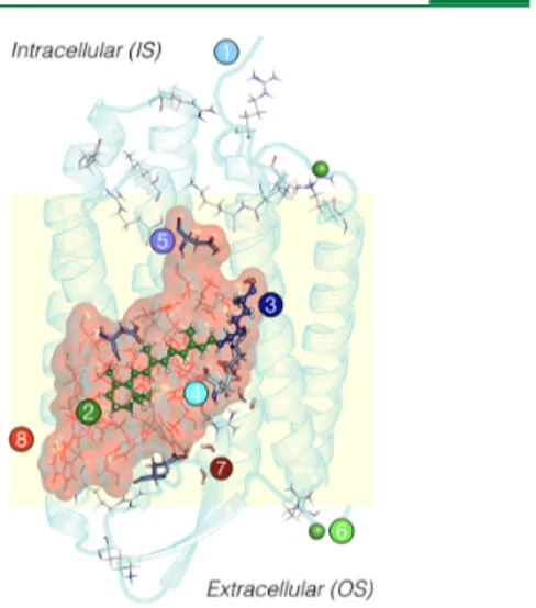
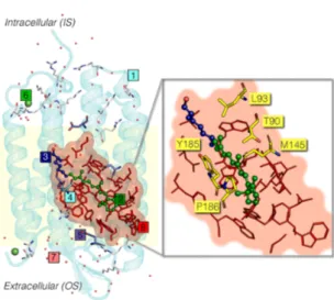
Figure 1.General scheme of a QM/MM ARM and a-ARM model, composed by (1) main chain (cyan cartoon), (2) chromophore rPSB (green ball-and-sticks), (3) Lys side chain covalently linked to the chromophore (blue ball-and-sticks), (4) main counterion MC (cyan tubes), (5) protonated residues GLH and ASH (violet tubes), (6) external Cl−(green balls) counterions, (7) water molecules (tubes), and the (8) residues of the chromophore cavity subsystem (red frames). Parts 1 and 6 form the environment subsystem. Parts 2 and 3 form the Lys-QM subsystem, which includes the H-link atom located along the only bond connecting blue and green atoms. Parts 4 and 8 form the cavity subsystem. Water molecules (Part 7) may be part of the environment or cavity subsystems. The external OS and IS charged residues are shown in frame representation. Thisfigure, and all other protein structures presented in this work, were produced using PyMOL, version 1.2.59

DOI:10.1021/acs.jctc.9b00061 J. Chem. Theory Comput. 2019, 15, 3134−3152 3135

ionizable residues side chain, (C) placement of OS and IS counterions, and (D) congruous generation of single or multiple point mutations, allowing in principle for a faster and parallel model building. Such an automated approach, called a-ARMdefault, adopts a set of default values for the choices

determining how the QM/MM model is built. These are chain A, if different chains are present in the crystallographic data; chromophore cavity generation based on Voronoi tessellation and alpha spheres theory and including the lysine residue covalently linked to the rPSB, plus the main (MC) and secondary (SC) chromophore counterion residues; protonation states of the ionizable residues based on partial charges calculated at the crystallographic pH and using neutral His residues with theδ-nitrogen of the imidazole protonated (HID tautomer); OS and IS counterion (Na+_/Cl−_{) positions}

optimized with respect to an electrostatic potential grid constructed around each charged OS and IS residue.

Based on a benchmark set of 25 wild type rhodopsins (including vertebrate, invertebrate, and microbial) and 14 mutants and providing 39 observedλmaxa values, below we report

that a-ARMdefaulthas a 32/39 success ratio in reproducing the

observedλmaxa trend. In the cases for which the fully automated

protocol fails (i.e., produces ΔES1−S0 values far from the

observed ones), we show that a semiautomatic approach called a-ARMcustomizedcan be employed, allowing for the construction

of customized models, which display consistency with the observed trend.

Both a-ARMdefaultand a-ARMcustomizednot only have a high

level of automation with respect to the original ARM, but also greatly reduced input preparation time, higher accuracy even when considering distant rhodopsins, andfinally full reprodu-cibility of thefinal results.

2. THEORY AND IMPLEMENTATION OFa-ARM

a-ARM is an improved version of the original ARM based on a Python subroutine, which allows for an automated production of QM/MM models of the type described inFigure 1. a-ARM is designed to generate the ARM input therefore avoiding, as much as possible, human manipulations. In a sense, a-ARM incorporates the original protocol but provides automatically (but also semiautomatically) all required input information. In order to facilitate the description of how a-ARM works, in

section 2.1we revise the main feature of the original input. The followingsections 2.2and2.3deal with the a-ARM structure and

section 2.4deals with a-ARM benchmarking.

2.1. ARM Input: Assets and Limitations. The original ARM is, substantially, a Bash shell script that links a series of publicly available computational packages, by automatically managing and passing information between them. The input (herein called ARM input) is constituted by twofiles containing the information described in points A−D ofsection 1. The PDBARM_{inputfile contains the protein structure in PDB format}

(from either crystallographic or comparative modeling data) with the assigned residue protonation states and positions of Na+_/Cl− _{external counterions. Instead, the cavity input file}

contains a list of residues constituting the cavity where the chromophore resides.

In the workflow of the protocol shown inFigure S1of the Supporting Information, the ARM input is treated sequentially to perform the following actions by a series of software packages: mutation and rotamer selection, using SCWRL4;60addition of waters and hydrogens, employing DOWSER;61 MM energy minimization and simulated annealing (SA)/molecular

dynam-ics (MD) relaxation, with GROMACS;62 geometry optimiza-tion and energy reevaluaoptimiza-tion at the CASSCF(12,12)/AMBER and CASPT2(12,12) levels, respectively,48using a combination of the quantum chemical package MOLCAS63and molecular mechanics package TINKER.64 The SA/MD procedure is performed starting with N = 10 different seeds that provide 10 independent sets of initial velocities for generating 10 independent QM/MM models. Therefore, the resulting output files include 10 replicas of the final equilibrated ARM model as well as the average vertical excitation energy, from now on called simply vertical excitation energy (ΔES1−S0), between ground

state (S0) and thefirst singlet excited state (S1) computed at the

CASPT2 level. From these 10 models, the output structure characterized byΔE_S1−S0values closest to the average (N = 10) is selected. As anticipated above, such models correspond to gas-phase and globally uncharged models of a rhodopsin monomer, composed of three subsystems, i.e., environment, cavity, and Lys-QM (seeFigure 1). The QM part of the Lys-QM subsystem is treated at the CASSCF level and corresponds to the rPSB chromophore, while the Lys part of the same subsystem as well as the environment and cavity subsystems correspond to the MM part of the model and are described at the AMBER level. The entire model construction and 3-root state-average CASPT2(12,12) vertical excitation energy calculation takes, after the inputfile preparation, ∼36 h CPU time when running the 10 replicas in parallel on a modern workstation.

In spite of their elementary structure, ARM models have been shown to be able to reproduce trends inλmaxa variation in a set of

diverse rhodopsins.52 In addition, further studies have demonstrated that the same models are able to successfully simulate, thanks to CASSCF gradients, properties associated with rhodopsinfluorescence,20,55and photoisomerization.65−67 However, as mentioned insection 1, a critical automation limit of ARM is related to the manual preparation of its inputfiles. Such preparation takes time (seesection S1in the Supporting Information). In our experience, we found that a skilled user can complete the preparation of an ARM input for a new rhodopsin protein in not less than 3 h.

Thefirst step in the manual preparation of an ARM input is the manipulation of the PDB file containing the original rhodopsin crystallographic structure (see point A ofsection 1), aimed at removing unnecessary information such as unwanted protein chains and subsequently adjusting atoms and residue numbering. This step will also deal with the possible presence of two alternate locations of selected side chains in the same PDB file, for which there is no established selection procedure. Related to this issue, also selection of the residue containing the retinal chromophore (i.e., the residue that will define the Lys-QM subsystem) has to be performed manually. The selected protein chain, side-chain rotamers, and chromophore residue are ultimately written in the PDBARM_file.

ARM models are sensitive to the correct choice of protonation state of the protein ionizable residues52(see point C ofsection 1). To perform such an assignment, one may use experimental data and/or execute the external program PROPKA68(see also

section 2.2.3) and analyze its output. In this way, residues with uncommon protonation states are identified and their three-letter code manually written in the PDBARM_file.

The location of the residues belonging to the cavity surrounding the retinal chromophore (see point B ofsection 1) is also performed manually through an external Web-based tool (CASTp,69 see section 2.2.2). The user has then to manually prepare the cavityfile containing the list of the selected

DOI:10.1021/acs.jctc.9b00061 J. Chem. Theory Comput. 2019, 15, 3134−3152 3136

cavity residues. Finally, the last step of the ARM input preparation is the neutralization of the protein environment, through the distribution of OS and IS counterions (see point D ofsection 1). This step is the most time-demanding and does not follow a well-defined procedure, since it requires the visual inspection of the protein structure and, therefore, has an impact on the reproducibility of the generated model. Again, thefinal type and coordinates of the selected counterions are added to the PDBARM_{file. For a more detailed description of the above}

steps seesection S1in the Supporting Information.

2.2.a-ARM. As already mentioned above, a-ARM has the ability to operate either as a fully automated tool or as an

interactive system for the semiautomatic generation of the ARM input presented above. More specifically, in a-ARM the information required for generating complete PDBARM _and

cavityfiles may be provided via either default choices or by answering specific questions in the command line of terminal window. With such an input, the QM/MM model generated by the subsequent calculation is called a-ARM model.

According to the general workflow of a-ARM (seeFigure 2), the procedure starts with the selection of the rhodopsin structure of interest used to prepare the ARM input and ends with the generation of the QM/MM a-ARM model and the calculation of theΔES1−S0and correspondingλmaxa (throughout Figure 2.a-ARM workflow. After the selection of the protein chain, a-ARM generates the ARM input files with complete information on the chromophore cavity, protonation states, and counterion placement (seeFigure 1) corresponding to points B−D ofsection 1. The input is then used for the execution of the original ARM,52_{obtaining as output 10 a-ARM models along with the calculated average vertical excitation energy (ΔES1−S0). The} parallelograms represent input or output data, the continuous line squares refer to processes or actions, and the dashed lines mean software executions. The [A] mark symbolizes fully automation, whereas the [M] mark represent manual decision. Finally, the [M/A] mark indicates situation that may be either manual or automated (see text). Notice that the software execution labeled“QM/MM calculation” is the same as in the original ARM (see ref

52). In a-ARM the production of the PDBARM_{and cavity inputfiles takes only a few minutes.}

DOI:10.1021/acs.jctc.9b00061 J. Chem. Theory Comput. 2019, 15, 3134−3152 3137

this work, we assume that the vertical excitation energy provides a good approximation for the energy corresponding to theλmaxa at

the CASPT2 level of theory). The code behind the workflow reported in Figure 2 is driven by a modular, Python-based collection of routines and can be accessed upon request to the authors. In the following, we detail the four steps (seesections 2.2.1−2.2.4) of the a-ARM workflow. Insection 2.2.5, we will instead report on an automatic mutant generation method also currently incorporated in a-ARM.

2.2.1. Step 1. Automatic Identification of Protein Chain, rPSB, Chromophore Bounded Lys, MC, and SC. In Step 1 of

Figure 2(see alsoFigure S2in the Supporting Information) we display the workflow necessary to obtain the initial structure of the rhodopsin of interest. To begin with, the user has the option to provide a crystallographic structure or a comparative model in PDB format or type the PDB ID to download thefile directly from the RCSB PDB.57The program is then able to identify automatically the different protein chains, which may be present in the PDBfile and select chain A by default (i.e., automatically or [A]) or, alternatively, let the user select the chain (i.e., manually [M]). Thus, the program generates afile PDB(i)ARM,

which contains information on the selected chain, residue conformations, chromophore, and water molecules.

Due to their localflexibility, certain residues may have two alternate side chains locations (i.e., conformations) in the protein crystallographic structure. The strategy adopted to assign a single rotamer, without the need to visualize the structure, is to analyze the atom occupancy number in the coordinate section of thefile. This parameter, which takes values from 0 to 1, is used as a criteria to estimate the frequency of each conformation. Accordingly, a-ARM identifies the residues with atom occupancy different from 1.0, creates a list with residue name and sequential number, and the occupancy value of the alternate side chain locations and acts automatically [A] by selecting the rotamer with the largest occupancy or, alter-natively, asks the user to select the wanted rotamer by typing the corresponding number [M].

The rPSB chromophore is automatically recognized and selected. For this purpose, the program identifies all residues which are not standard amino acids, waters, and membrane lipids and generates a list of possible chromophores. Once again, the chromophore can be selected automatically by default, which corresponds to the ordinary rPSB chromophore [A], or the user may select the correct option manually by typing the corresponding residue number [M]. Here, we should stress that, while this step is instrumental for a future generalization of a-ARM (e.g., for considering multiple chromophores), there is only a single rPSB chromophore in rhodopsins and therefore the user intervention is not needed. Moreover, although in the majority of rhodopsin coordinatefiles in the RCSB PDB,57the retinal and the covalently linked lysine are two distinct residues (i.e., RET and LYS, respectively) in a minority of cases (e.g., 6EID70and 6EIG70) retinal and lysine constitute a single residue (LYR). In principle, this LYR formatting is not compatible with ARM52algorithms, which are designed to recognize the RET and linker LYS as distinct residues. To deal with that, a-ARM is now able to automatically recognize the LYR residue and subsequently split it into RET and LYS, respecting the standard format of residue and atom names (see section S4 in the Supporting Information).

Another important feature of the program is that, based on the geometrical parameters of the selected chromophore, the chromophore-linked Lys side chain and the potential MC and

SC counterions are automatically identified. This is achieved by first locating the linked Lys as the residue geometrically closest to the chromophore, by computing the Euclidean distance between each atom in the chromophore and the coordinates of the nitrogen“NZ” of all the Lys residues present in the structure. Then, the MC and SC are identified as the two Asp and/or Glu and/or crystallographic Cl−residues geometrically closest to the chromophore-linked Lys side chain, by computing the distance between the coordinates of its nitrogen “NZ” and the coordinates of the oxygen “O” of each of the carboxylate-bearing residues (or the chlorine atom). However, this selection is only preparatory to the ionization state assignment (see

section 2.2.3) that determines if the SC and MC are indeed acting as negatively charged Schiff base counterions. The inclusion of the Cl−anions contained in the X-ray structure into the QM/MM model, even when not considered as MC or SC, is a new feature of a-ARM that allows a more realistic description of rhodopsin chloride pumps (i.e., 5B2N71and 5G2872).

2.2.2. Step 2: Automatic Generation of the Chromophore Cavity. The identification and characterization of the chromophore cavity is a key step for the definition of congruous QM/MM models of rhodopsins (seeFigure 2andsection 2.1). There are different algorithms for protein pocket detection.73 These are mainly available via Web server-based facilities, but a few are distributed as a code for local usage. The widely used Web servers include CASTp,69_{employed in the original ARM} protocol.52Even though CASTp has proven to be effective, the fact that it is not available as a command line code makes it unsuitable for a full automation. Thus, we decided to use the Fpocket software,74 which can be integrated in a-ARM as illustrated inFigure 2(see also Figure S3in the Supporting Information). Fpocket detects the chromophore cavity based on Voronoi tessellation and alpha spheres built on top of the publicly available package Qhull.74 First, a-ARM receives as input the previously generated PDB(i)ARMfile and automatically

executes the Fpocket software using the default options.74As output, several protein pockets are obtained along with their scores. The selected chromophore cavity is the one that contains the Lys covalently linked to the rPSB and has the highest score. Finally, the previously identified MC and SC counterion residues are added to the cavity list (if not already present) and the updated list is written in thefinal cavity file.

2.2.3. Step 3: Automatic Assignment of Ionization States. Our procedure for the assignment of the protonation state of the ionizable residues at a given pH and in their specific protein environments is based on the assumption that such state is a function of the pKavalue.75Accordingly, each residue with a

titratable group is associated with a model pKavalue (pKaModel),76

interpreted as the pKadisplayed when the other protein side

chains are in their neutral state. On the other hand, pKaModelis

affected by the interaction between the residue and its actual environment, causing a change from the model value to the real pKavalue (seeeq 1) called pKaCalc. The magnitude of this change,

called shift value (ΔpKa), depends on the presence of hydrogen

bonds, desolvation effects, and Coulomb interactions, all modulated through the degree to which the ionizable residue is“buried” within the protein.68,75

= + Δ Δ = −

K K K K K K

p _aCalc p _amodel p _a; p _a p _aCalc p _amodel

(1)

The adopted procedure is outlined in Step 3 ofFigure 2(see also Figure S4 in the Supporting Information), and it is initialized automatically after the detection of the PDB(i)ARMand DOI:10.1021/acs.jctc.9b00061 J. Chem. Theory Comput. 2019, 15, 3134−3152 3138

cavity files. In case that the crystallization conditions are available in the initial PDB structurefile, the program identifies the experimental pH making the pH selection automatic [A]. Otherwise, the user is asked to insert the pH value and the pH selection is thus not automatic [M]. Once the working pH is assigned, the pKaCalcis obtained using the PROPKA software

which also determines the burying percentage.68A preliminary preparation of the PDB(i)ARMfile, consisting of completing the

heavy missing atoms of chain residues (including hydrogen atoms), is needed to guarantee the correct operation of PROPKA.77This requires using the PDB2PQR78,79software, which operates under the following workflow: (i) check for missing heavy atoms, (ii) reconstruct heavy atoms, (iii) build and optimize hydrogens, and (iv) assign atomic parameters (for further details see ref78). PDB2PQR is automatically launched using as input the PDB(i)ARMfile and as arguments the given pH

and the AMBER forcefield. After that, PROPKA is launched and its output contains information on the calculated (pKaCalc) values

for each ionizable residue in the protein at the given pH.68_The subsequent assignment of the protonation states of the ionizable groups is carried out based on the above information.

According to a first approach (not reported in Figure 2) employed by Melaccio et al.52for the construction of the original ARM models, the parameters used to identify the state of the ionizable residues are the burying percentage, which indicates how accessible the residue is from the surface (for further details see ref68), and theΔpKashift calculated at pH 7.0 as shown in eq 1. In contrast, in a-ARM the parameter used to identify the state of the ionizable residues is the side-chain ionization equilibrium. Such equilibrium is estimated by inserting both the pKaCalcvalue and the established working pH in the Henderson−

Hasselbalch equation,80 _{which describes the relationship} between the pH and the pKaand the equilibrium concentrations

of dissociated [A−] and non-dissociated acid [HA], respec-tively:80−82 = K + _{[ ]}[ ]− pH p log A HA aCalc (2)

The charges of the positive and negatively ionizable residues are then deduced fromeq 2using the following approximated rules:81 ⌈ ⌉ = − + − − − Q ( 1) 1 10

; for Asp and Glu

K (pH p a ) Calc (3) and ⌈ ⌉ = + + + + − Q ( 1) 1 10

; for Arg, Lys, and His

K

(pH p aCalc) ₍₄₎

where⌈Q+_{⌉ and ⌈Q}−_{⌉ are integers obtained by rounding the}

decimals using the“round half to even” convention. Once ⌈Q+_⌉

and⌈Q−⌉ are obtained, the following criteria is used to assign the ionization (i.e., protonation) state:

= ⌈ ⌉ = − ⌈ ⌉ ≠ − ⌈ ⌉ = + ‐ ⌈ ⌉ ≠ + − − + + l m ooooo oooo n ooooo oooo Q Q Q Q protonation state Asp, Glu, if 1 ASH, GLH, if 1

Arg, Lys, His, if 1

ARN, LYD, HIE HID, if 1 ₍₅₎

Thefinal result is added to the file PDB(i)ARMto generate thefile

PDB(ii)ARMnow also containing the ionization states.

There are two aspects that limit the confidence in the automation of the ionizable-state assignment described above. Thefirst is that, due to the fact that the information provided by PROPKA68is approximated, the computed pKaCalcvalue may, in

certain cases, be not sufficiently realistic. The second aspect concerns the assignment of the correct tautomer of histidine. This amino acid has charge of +1 when both theδ-nitrogen and ϵ-nitrogen of the imidazole ring are protonated (HIP), while it is neutral when either theδ-nitrogen (HID) or the ϵ-nitrogen (HIE) are deprotonated. a-ARM uses as a default the HID tautomer for the automatic assignment [A] or allows the user to choose between the three tautomers for a non-automated selection [M]. Therefore, when possible, the user should collect the available experimental data and/or inspect the chemical environment of the ionizable residues including the histidines and propose the appropriate tautomer. Further details are given insection S8in the Supporting Information.

2.2.4. Step 4: Automatic Counterion Placement. The procedure to select and place OS and IS counterions in the model represents a difficult automation problem (seesection 2.1). Herein, we report a novel approach for automatically generating and placing such counterions and therefore avoiding user manipulation. The approach is documented in Step 4 of

Figure 2(see alsoFigure S5of the Supporting Information). The initial task consists in determining the type (Cl−and/or Na+) and number of counterions needed to neutralize the protein environment. This calculation is carried out based on the actual charges of the OS and IS surfaces, which depend on the quantity of positively and negatively charged residues. Therefore, the output of Step 4 depends on the result of Step 3.

To define the OS and IS surfaces, the protein is oriented along the z axis, as illustrated inFigure 3. To this aim, the protein coordinates found in the PDB(ii)ARMfile are first centered at the

protein center of mass (xyzcm). The new set of coordinates are then rotated such as the main rotational axis is aligned with the z axis, using the Orient utility of the VMD83software. Finally the coordinates are recentered at the center of mass of the chromophore. These coordinate transformations allow to define

Figure 3.External counterion placement. Schematic representation of the procedure for the definition of the number and type of external counterions needed to neutralize the IS (A) and OS (B) surfaces of bovine rhodopsin. We also illustrate the grid generated by the PUTION code to calculate the coordinates of the Cl−counterions in the IS (C) and the Na+_{in the OS (D). The negatively and positively charged} residues are illustrated as red and blue sticks, respectively, and the Na+ and Cl−counterions as blue and green spheres, respectively.

DOI:10.1021/acs.jctc.9b00061 J. Chem. Theory Comput. 2019, 15, 3134−3152 3139

an imaginary plane orthogonal to the z-axis and containing the z coordinate of the NZ atom (zPSB_{) of the rPSB moiety. Such a}

plane divides the protein in two halves and establishes the OS and IS surfaces in terms of the z value: the ionized residues with a z value larger than zrPSB

belong to the OS surface, whereas those residues with z lower or equal to zrPSB_{belong to the IS surface.}

The charge of each surface (QOS, QIS) is calculated as the

difference between the number of positively charged (Arg, Lys, and His) and negatively charged (Asp, Glu, and crystallographic Cl−anions) residues. Once the surface charge is known, the protocol provides the type and number of counterions required to neutralize the net charge of each surface independently and, in turn, of the full protein. This procedure is illustrated inFigure 3A,B for the case of bovine rhodopsin (Rh).84_{Accordingly, the} net charge of the IS surface is QIS= +6, resulting from 16

positively charged and 10 negatively charged residues, whereas the net charge of the OS is QOS=−2, given by 7 positively

charged and 9 negatively charged residues. As a consequence, 6 Cl−and 2 Na+must be added to compensate the positive and negative charge of the IS and OS, respectively.

One main difference between the original ARM and the new a-ARM protocol is that, whereas the original version requires the visual inspection of the PDBfile to manually identify the charged residues and calculate the number and identity of the counterions to be added on each surface, the new version performs these tasks automatically. The automatic location of ionized residues on OS and IS provides the basis to properly and automatically place the counterions.

As described for the original ARM,52the user-defined OS and IS surfaces are neutralized using a set of counterions placed, semiautomatically, in the regions where thefield generated by the charge of the ionized residues is stronger. In fact, while ARM employs a program called PUTION (described by Melaccio et al. as the ION Module52) that uses an energy minimization procedure to place the counterions, the user has to manually specify the target residues on the IS and OS surfaces, including number of residues, residue number identification, and the number and type of counterions to be added. With the aim of removing the above automation limits, a-ARM adopts a different strategy to assign the target residues and execute PUTION automatically. More specifically, PUTION optimizes the counterion positions on the basis of the Coulomb’s law,85_by computing an electrostatic potential grid constructed around all charged residues and excluding points whose distance is larger than 8.0 Å from the center of charge of a ionized residue and shorter than 2.0 Å from any residue atom.

As reported in Step 4 of Figure 2, the PUTION code is automatically launched right after the determination of the partial charges of each residue (see previous section). The program starts by placing a counterion on the surface with the highest net charge. The placement process is then alternated between the OS and IS surfaces, until both are neutralized. The energy of the Nth counterion is computed from the electrostatic interaction with the protein and the N − 1 preceding counterions. As an output, the geometry of all external counterions is generated as illustrated in Figure 3C,D and added to PDB(ii)ARMto generate thefinal PDBARMfile, which is

ready to be used as an input for the QM/MM model building. 2.2.5. Automatic Generation of Mutants: Redefinition of Cavity, Ionization States, and Counterion Placement. By exploiting the backbone-dependent rotamer library imple-mented in the software SCWRL4,60the original ARM has the ability to perform amino acid substitutions on rhodopsin

structures and generate QM/MM models of mutants.52 However, such calculation has serious limitations, since the generated mutants tend to preserve the chromophore environ-ment (i.e., chromophore cavity, protonation states, and external counterions) of the wild type form (unless this information is manually modified). Therefore, although the method has been shown to be effective when a wild type residue is substituted with a residue with the same charge,52 it is unsuitable for replacements altering the residue charge or polarity, thus possibly affecting the protonation state of nearby residues and, in general, the distribution of OS and IS counterions. An additional problem with the original ARM is that when a mutated residue does not belong to the chromophore cavity, this is not relaxed but kept frozen.

Given the importance of developing a suitable tool for the construction of congrous QM/MM models of mutants, we implemented in a-ARM a new mutation method that takes into account the effects of amino acid substitution on the protein environment (see the workflow in Figure 4). The method requires an additional inputfile with a .seqmut extension that contains the information on the type (single, double, triple, etc.) and number (N in the flowchart of Figure 4) of required mutations. After detecting the .seqmutfile, a-ARM generates N lists with information on each mutation (mutnin theflowchart of Figure 4). Each list, along with the PDB(i)ARMgenerated for the

wild type structure in Step 1, provides the input for the automatic execution of the SCWRL4 software. In the case of multiple mutations, the SCWRL4 software is re-executed. When the mutation process is concluded, the mutant QM/MM models are built through generation of the cavity, assignment of protonation states, and selection of counterion placement carried out by following Steps 2−4, as described above for the wild type structure. Notice that in Step 2 the mutated residues are always included in the cavity subsystem (MM part) and, consequently, they are relaxed during the SA/MD procedure and subsequent QM/MM level geometry optimization.

2.3. a-ARMdefault and a-ARMcustomized Approaches. In Figure 2, we marked as automatic [A] or manual [M] the choices in Steps 1−4 described insections 2.2.1−2.2.4. The [A] or [M] choices define two different approaches for the generation of a-ARM models. Thefirst, named a-ARMdefault, is a fully automated

approach that delivers maximum input preparation speed (see

section 3.1) for the systematic building of a-ARM models and, therefore, useful for the generation of large arrays of wild type rhodopsins and of their mutants (as described insection 2.2.5). This is achieved by employing the default choices described in

sections 2.2.1−2.2.4. Accordingly, these models are built on the basis of chain A and the side-chain rotamer with the highest occupancy, a chromophore cavity generated by Fpocket and including the Lys covalently linked to the rPSB and MC and SC residues, ionization states predicted at the crystallographic pH (or at physiological pH 7.4 in the case of no experimental information available) with a neutral HID tautomer of histidine and automatic counterion placement decided by the PUTION code.52In addition to these choices, a default choice has to be taken for the rhodopsins displaying, for certain residues, alternate side chain locations with exactly the same top occupancy. As we will see below, this is found in two crystallographic structure of our benchmark set (seesection 2.4) where two rotamers display a 50% probability (occupancy number 0.5) to contribute to the observed structure. In this situation, the default action of the automated a-ARMdefault

approach is to generate one a-ARM model for each rotamer.

DOI:10.1021/acs.jctc.9b00061 J. Chem. Theory Comput. 2019, 15, 3134−3152 3140

The second approach, named a-ARMcustomized, is

semi-automatic and slower than a-ARMdefault but of increased

accuracy (seesection 3.2). In fact it allows, for instance, the construction of“customized” a-ARM models useful when the default choices give a poor result in terms of reproducing the experimentalΔES0−S1trends (e.g., differences with experimental

data larger than 3−4 kcal mol−1_{; 0.1−0.2 eV). a-ARM} customized

requires user manipulation during Steps 1 and 3, which consists of selecting the protein chain (in case of multi-chain rhodopsins), typing the number identifier of ionizable residues with neutral charge (based on chemical criteria or experimental data), and selecting the tautomer of the histidine. Instead, Steps 2 and 4 are performed as in the a-ARMdefaultapproach. Notice

that even though the semiautomatic procedure requires user

manipulation, the resulting models are always replicated even when different users select the options.

2.4. Benchmark Set fora-ARM. Insections 2.2and2.3, we have mainly dealt with the automation, speed, and reproduci-bility of a-ARM. However, no information is provided on the protocol accuracy in predicting property trends and, at the same time, on the transferability of the a-ARM model between rhodopsins with diverse (i.e., non-homologous) sequences. Information on both accuracy and transferability requires a benchmark study that, here, we limit to the calculation of ΔES1−S0. In order to compare this computed quantity with the

experimental data, we assume that the observedΔES1−S0values

can be derived from the observedλmaxa via the equationΔES1−S0=

hc/λmaxa . As mentioned above, the calculated values are obtained

via single-point 3-roots state-average CASPT2(12,12)// CASSCF(12,12)/AMBER calculations yielding the potential energy of the S0, S1, and S2 states. The fact that ΔES1−S0

corresponds to an allowed electronic transition is supported via oscillator strength ( fOsc) calculations.

A benchmark data set comprising a pool of observedλmaxa

(expressed in terms ofΔES0−S1) values for 25 wild type and 14

mutant rhodopsins was employed for testing a-ARM. From these mutant rhodopsins, only 2 have an available X-ray structure (i.e., ASRAT-D217E and ChR2-C128T), while the

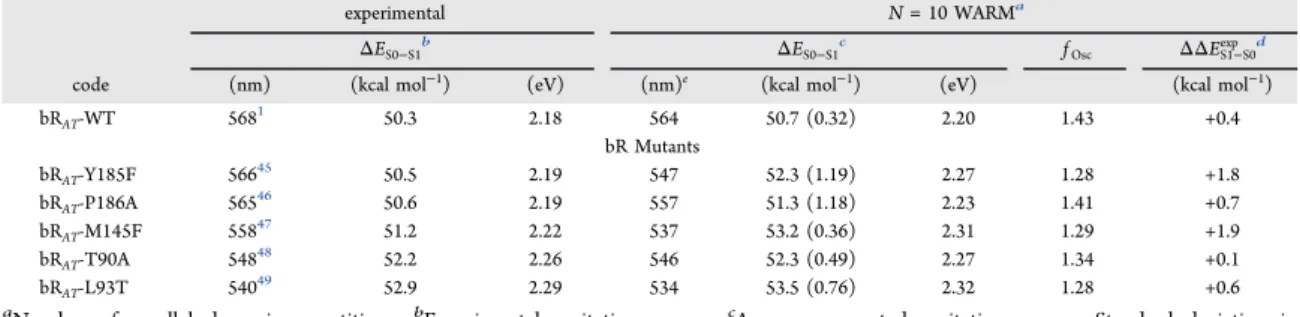
other 12 were generated by the procedure described insection 2.2.5. The data set incorporates the set employed by Melaccio et al.52for testing the original ARM (m-set), an additional set of rhodopsins (a-set), and a set of Rh mutants (Rh mutants). The full set, which includes vertebrate, invertebrate, and microbial rhodopsins is presented inTable 1and features λmaxa values

ranging from 430 to 575 nm. The number of observedλmaxa

values will provide information on the method accuracy while the diversity (e.g., microbial vs vertebrate) of rhodopsins will provide information on the transferability of the generated models.

In our benchmark study, we initially use the a-ARMdefault

approach to obtain, in a fully automated fashion, theΔES0−S1

trend. However, as reported in the previous section, default choices do not always generate a single a-ARM model. As we will document insection 3.2, this happens for the ASRAT, ASR13C,

and KR2 rhodopsins. In these cases, the selection of a single representative rotamer is only possible when the corresponding observedΔES0−S1value is available (as for our benchmarks). The

selected a-ARM model will be the one yielding the computed ΔES0−S1value closest to the observed one.

3. RESULTS AND DISCUSSION

We are interested in answering the question of whether the a-ARM models generated using the inputfiles PDBARM_{, cavity, and}

seqmut are suitable for predicting trends ofΔES1−S0of wild type

and mutant rhodopsins. For this purpose, wefirst compute the trend generated using the fully automated a-ARMdefault

approach. Then, we describe some specific models that do not produce values consistent with the observed trend (i.e., with deviations larger than∼3−4 kcal mol−1), for which the use of a-ARMcustomizedis needed. We recall that, in all cases, the computed

ΔES1−S0 values are averages over 10 replicas of the final

equilibrated a-ARM model (seesection 2.1). The S0 and S1

energies, for each of the 10 replicas, are reported inTable S3in the Supporting Information.

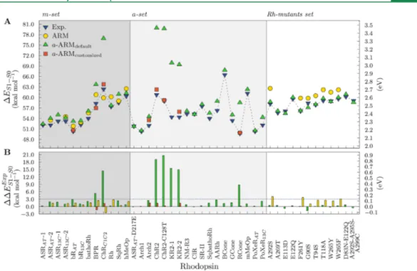
3.1.a-ARMdefault.Figure 5A displays theΔES1−S0values for

the 25 wild type and 14 mutant rhodopsins of the benchmark set (see Table 1), using the a-ARMdefault approach described in Figure 4.Automatic generation of mutants by using the SCWRL460

software. The code does not require any interaction with the user during execution.

DOI:10.1021/acs.jctc.9b00061 J. Chem. Theory Comput. 2019, 15, 3134−3152 3141

section 2.3(green up triangles), whereasFigure 5B displays their differences calculated with respect to experimental data (ΔΔES1−S0Exp ). The numerical values together with the

corre-spondingλmaxa and transition oscillator strength ( fOsc) values are

given inTable 2and demonstrate that the S1state is indeed a

strongly absorbing state.

Before discussing the performance of the fully automated approach, it is necessary to explain whyFigure 5shows, for certain rhodopsins, results from more than one model.

According to the a-ARMdefaultapproach (seesection 2.3), this

occurs for rhodopsins whose crystallographic data contain two alternate locations of some side chains. Multiple rotamers are found in the 1XIO,863X3C,1026G7H,87and 6EID70 crystallo-graphic structures. In the 1XIO structure, corresponding to Anabaena sensory rhodopsin (ASR), two possible conforma-tions were identified for both residues Lys-310 (ALys and BLys) and RET-301 (all-trans and 13-cis rPSB) that form the Lys-QM subsystem. Each rotamer in each pair exhibits 50% probability Table 1. Benchmark Set of Wild Type and Mutant Rhodopsinsa

proteinb _{code PDB ID RET-C}c _{chain(s) λ}

max

a _ΔE S0−S1

m-Set

X-ray Crystallographic Structures

Anabaena sensory rhodopsin (M) ASRAT 1XIO

86 all-trans A 550 52.0 (2.25)86 ASR13C 1XIO 86 13-cis A 537 53.2 (2.31)86 Bacteriorhodopsin (M) bRAT 6G7H87 all-trans A 568 50.3 (2.18)2 bR13C 1X0S88 13-cis A 548 52.2 (2.26)2 Bathorhodopsin (V) bathoRh 2G8789 all-trans A, B 529 54.0 (2.34)90,91 Blue proteorhodopsin (M) BPR 4JQ692 all-trans A, B, C 490 58.3 (2.52)93

Bovine rhodopsin (V) Rh 1U1984

11-cis A, B 498 57.4 (2.49)32,91

Chimaera channelrhodopsin (M) ChRC1C2 3UG9

94

all-trans A 458 62.4 (2.71)40

Squid rhodopsin (I) SqRh 2Z7395

11-cis A, B 489 58.5 (2.54)96

Comparative Models

Human melanopsin (V) hMeOp 2Z73e _{11-cis A 473 60.4 (2.62)}d

a-Set

X-ray Crystallographic Structures

Anabaena sensory rhodopsin D217E (M) ASRAT-D217E 4TL3

97

all-trans A, B 552 51.8 (2.25)98

Archaerhodopsin-1 (M) Arch1 1UAZ99 all-trans A, B 568 50.3 (2.18)100

Archaerhodopsin-2 (M) Arch2 3WQJ101 all-trans A 550 52.0 (2.25)101

Channelrhodopsin-2 (M) ChR2 6EID70

all-trans A, B 470 60.8 (2.64)70

Channelrhodopsin-2 N24Q/C128T (M) ChR2-C128T 6EIG70

all-trans A, B 485 59.0 (2.56)70

Krokinobacter eikastus rhodopsin 2 (M) KR2 3X3C102

all-trans A 525 54.5 (2.36)102

Nonlabens marinus rhodopsin-3 (M) NM-R3 5B2N71

all-trans A 517 55.3 (2.40)71

ClR 5G2872

all-trans A 517 55.3 (2.40)72

Sensory rhodopsin II (M) SRII 1JGJ103

all-trans A 497 57.5 (2.49)103

Squid bathorhodopsin (I) SqbathoRh 3AYM104

all-trans A, B 530 53.9 (2.34)104

Comparative Models

Ancestral archosaur rhodopsin (V) AARh 1U19e _{11-cis A 508 56.3 (2.44)}19

Human blue cone (V) BCone 1U19e _{11-cis A 430 66.5 (2.88)}105

Human green cone (V) GCone 1U19e 11-cis A 535 53.4 (2.32)105

Human red cone (V) RCone 1U19e 11-cis A 575 49.7 (2.15)105

Mouse melanopsin (V) mMeOp 2Z73e 11-cis A 467 61.2 (2.65)106

Parvularcula oceani Xenorhodopsin (M) PoXeRAT 4TL397,e all-trans B 568 50.3 (2.18)107

PoXeR13C 4TL3e 13-cis B 549 52.1 (2.26)107

Rh Mutants Set

Bovine rhodopsin mutation (V) A292S 1U19e _{11-cis A 491 58.2 (2.52)}32

A269T 1U19e _{11-cis A 514 55.6 (2.41)}43

E113D 1U19e _{11-cis A 510 56.1 (2.43)}108

E122Q 1U19e _{11-cis A 480 59.6 (2.58)}109

F261Y 1U19e _{11-cis A 510 56.0 (2.43)}43

G90S 1U19e _{11-cis A 489 58.5 (2.54)}110

T94S 1U19e _{11-cis A 494 57.9 (2.51)}111

T118A 1U19e _{11-cis A 484 59.1 (2.56)}112

W265F 1U19e 11-cis A 480 59.6 (2.58)113

W265Y 1U19e 11-cis A 485 59.0 (2.56)110

D83N-E122Q 1U19e 11-cis A 475 60.2 (2.61)109

A292S-A295S-A299C 1U19e 11-cis A 484 59.1 (2.56)110

a

Experimental maximum absorption wavelength,λmaxa _{, in nm, andfirst vertical excitation energy, ΔES0−S1, in kcal mol}−1_{. Values ofΔES0−S1in eV are} also provided in parentheses.bVertebrate (V), invertebrate (I), and microbial (M).cRetinal conformation.dAverage of available experimental values in refs106and114.e_{X-ray structure template model. See the details of the comparative model construction insection S6of the Supporting} Information.

DOI:10.1021/acs.jctc.9b00061 J. Chem. Theory Comput. 2019, 15, 3134−3152 3142

(occupancy number 0.5) to contribute to the observed structure.86,115 Therefore, the favored rotamer cannot be selected based on their occupancy, and thus, a-ARMdefault

generates four models: the all-trans (ASRAT) models using

ALys (ASRAT-1) and BLys (ASRAT-2) and the 13-cis (ASR13C)

models with, again, ALys (ASR13C-1) and BLys (ASR13C-2), as

also done manually in previous studies.52,54,55,86,115Thefinal models are then assigned to be those yielding aΔE_S0−S1value closest to the ones observed experimentally. More specifically, for ASRAT, we have selected model ASRAT-1 since (i) both the

error and the standard deviation are lower than that observed for the second model (ASRAT-2), while (ii) the oscillator strengths

are practically the same (see Table 2). A similar argument applies to the case of ASR13Cwhere, however, the selected model

is ASR13C-2.

In the case of the 3X3C structure, corresponding to Krokinobacter eikastus rhodopsin 2 (KR2), two alternate conformations (AAsp and BAsp) are present for the MC residue Asp-116 with occupancy numbers 0.65 and 0.35, respectively, and two alternate conformations (AGln and BGln) for Gln-157, both with occupancy number 0.5 (see

Figure 6A). Given their occupancy numbers, a-ARMdefaultuses

AAsp-116 and generates two models relative to Gln-157: KR2-1, which includes AAsp-116 and AGln-157, and KR2-2, which includes AAsp-116 and BGln-157. KR2-2 is the chosen model, after comparing the computed and observedΔES0−S1values.

The 6G7H structure, corresponding to Bacteriorhodopsin (bR), contains alternate locations for Asp-104, Leu-109, and Leu-15. However, the default choice leads to the generation of a single model with the rotamers AAsp-104, 109, and

ALeu-15, since the occupancy numbers of these specific rotamers are 0.80, 0.54, and 0.57, respectively.

Figure 5.(A) Vertical excitation energies (ΔES1−S0) computed with a-ARMdefault(up triangles) and a-ARMcustomized(squares), along with reported ARM52(circles) and experimental data (down triangles). S0and S1energy calculations were performed at the CASPT2(12,12)//CASSCF(12,12)/ AMBER level of theory using the 6-31G(d) basis set. The calculatedΔES1−S0values are the average of 10 replicas (seeTable S3in the Supporting Information). (B) Differences between calculated and experimental ΔES1−S0(ΔΔES1−S0Exp _{). Values presented in kcal mol}−1_{(left vertical axis) and eV} (right vertical axis).

Figure 6.a-ARM models. Conformational (the occupancy factor of the rotamers Asp-116 and Gln-157 are presented in parentheses) and ionization state variability for KR2 [PDB ID 3X3C] (A), BPR [PDB ID 4JQ6] (B), RCone (C) [PDB ID template 1U19], bRAT[PDB ID 6G7H] with standard (D) and modified cavity (E). MC and SC are presented as cyan and violet tubes, respectively.

DOI:10.1021/acs.jctc.9b00061 J. Chem. Theory Comput. 2019, 15, 3134−3152 3143

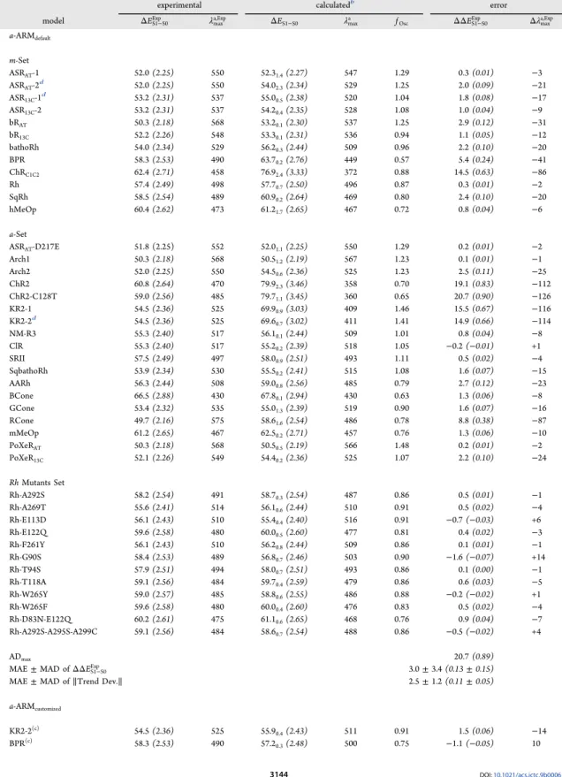
Table 2. Vertical Excitation Energies (ΔES1−S0, kcal mol−1and eV in Italic and Parentheses), Maximum Absorption

Wavelengths (λmaxa , nm), and Oscillator Strength (fOsc)a

experimental calculatedb _error

model ΔES1−S0Exp λmaxa,Exp ΔES1−S0 λmaxa fOsc ΔΔES1−S0Exp Δλmaxa,Exp

a-ARMdefault m-Set ASRAT-1 52.0 (2.25) 550 52.31.4(2.27) 547 1.29 0.3 (0.01) −3 ASRAT-2d 52.0 (2.25) 550 54.02.3(2.34) 529 1.25 2.0 (0.09) −21 ASR13C-1d 53.2 (2.31) 537 55.00.5(2.38) 520 1.04 1.8 (0.08) −17 ASR13C-2 53.2 (2.31) 537 54.20.4(2.35) 528 1.08 1.0 (0.04) −9 bRAT 50.3 (2.18) 568 53.20.1(2.30) 537 1.25 2.9 (0.12) −31 bR13C 52.2 (2.26) 548 53.30.1(2.31) 536 0.94 1.1 (0.05) −12 bathoRh 54.0 (2.34) 529 56.20.3(2.44) 509 0.96 2.2 (0.10) −20 BPR 58.3 (2.53) 490 63.70.2(2.76) 449 0.57 5.4 (0.24) −41 ChRC1C2 62.4 (2.71) 458 76.92.4(3.33) 372 0.88 14.5 (0.63) −86 Rh 57.4 (2.49) 498 57.70.7(2.50) 496 0.87 0.3 (0.01) −2 SqRh 58.5 (2.54) 489 60.90.2(2.64) 469 0.80 2.4 (0.10) −20 hMeOp 60.4 (2.62) 473 61.21.7(2.65) 467 0.72 0.8 (0.04) −6 a-Set ASRAT-D217E 51.8 (2.25) 552 52.01.1(2.25) 550 1.29 0.2 (0.01) −2 Arch1 50.3 (2.18) 568 50.51.2(2.19) 567 1.23 0.1 (0.01) −1 Arch2 52.0 (2.25) 550 54.50.6(2.36) 525 1.23 2.5 (0.11) −25 ChR2 60.8 (2.64) 470 79.92.3(3.46) 358 0.70 19.1 (0.83) −112 ChR2-C128T 59.0 (2.56) 485 79.71.1(3.45) 360 0.65 20.7 (0.90) −126 KR2-1 54.5 (2.36) 525 69.90.9(3.03) 409 1.46 15.5 (0.67) −116 KR2-2d _{54.5 (2.36) 525 69.6} 0.7(3.02) 411 1.41 14.9 (0.66) −114 NM-R3 55.3 (2.40) 517 56.10.1(2.44) 509 1.01 0.8 (0.04) −8 ClR 55.3 (2.40) 517 55.20.2(2.39) 518 1.05 −0.2 (−0.01) +1 SRII 57.5 (2.49) 497 58.00.9(2.51) 493 1.11 0.5 (0.02) −4 SqbathoRh 53.9 (2.34) 530 55.50.2(2.41) 515 1.08 1.6 (0.07) −15 AARh 56.3 (2.44) 508 59.00.8(2.56) 485 0.79 2.7 (0.12) −23 BCone 66.5 (2.88) 430 67.80.1(2.94) 430 0.63 1.3 (0.06) −8 GCone 53.4 (2.32) 535 55.01.3(2.39) 519 0.90 1.6 (0.07) −16 RCone 49.7 (2.16) 575 58.61.6(2.54) 486 0.78 8.8 (0.38) −87 mMeOp 61.2 (2.65) 467 62.50.2(2.71) 457 0.76 1.3 (0.06) −10 PoXeRAT 50.3 (2.18) 568 50.50.5(2.19) 566 1.48 0.2 (0.01) −2 PoXeR13C 52.1 (2.26) 549 54.40.2(2.36) 525 1.07 2.2 (0.10) −24 Rh Mutants Set Rh-A292S 58.2 (2.54) 491 58.70.3(2.54) 487 0.86 0.5 (0.01) −1 Rh-A269T 55.6 (2.41) 514 56.10.6(2.44) 510 0.91 0.5 (0.02) −4 Rh-E113D 56.1 (2.43) 510 55.40.4(2.40) 516 0.91 −0.7 (−0.03) +6 Rh-E122Q 59.6 (2.58) 480 60.00.5(2.60) 477 0.81 0.4 (0.02) −3 Rh-F261Y 56.1 (2.43) 510 56.20.8(2.44) 509 0.86 0.1 (0.01) −1 Rh-G90S 58.4 (2.53) 489 56.80.7(2.46) 503 0.90 −1.6 (−0.07) +14 Rh-T94S 57.9 (2.51) 494 58.00.7(2.51) 493 0.86 0.1 (0.00) −1 Rh-T118A 59.1 (2.56) 484 59.70.4(2.59) 479 0.86 0.6 (0.03) −5 Rh-W265Y 59.0 (2.57) 485 58.80.6(2.55) 486 0.88 −0.2 (−0.02) +1 Rh-W265F 59.6 (2.58) 480 60.00.4(2.60) 476 0.83 0.5 (0.02) −4 Rh-D83N-E122Q 60.2 (2.61) 475 61.10.6(2.65) 468 0.76 0.9 (0.04) −7 Rh-A292S-A295S-A299C 59.1 (2.56) 484 58.60.7(2.54) 488 0.86 −0.5 (−0.02) +4 ADmax 20.7 (0.89)

MAE± MAD of ΔΔES1−S0Exp 3.0± 3.4 (0.13 ± 0.15)

MAE± MAD of ∥Trend Dev.∥ 2.5± 1.2 (0.11 ± 0.05)

a-ARMcustomized KR2-2(c) _{54.5 (2.36) 525 55.9} 0.4(2.43) 511 0.91 1.5 (0.06) −14 BPR(c) _{58.3 (2.53) 490 57.2} 0.3(2.48) 500 0.75 −1.1 (−0.05) 10 DOI:10.1021/acs.jctc.9b00061 J. Chem. Theory Comput. 2019, 15, 3134−3152 3144

Furthermore, in the case of 6EID structure, corresponding to Channelrhodopsin-2 (ChR2), two alternate locations exist for the rPSB LYR: ALYR and BLYR, with occupancy numbers of 0.70 and 0.30, respectively. Therefore, the default model was generated using the conformation ALYR. This choice is consistent with the all-trans configuration of the rPSB presented in the resting conformation of ChR2.70

In the following sections, when discussing the results of ASRAT, ASR13C, and KR2, we will solely consider the models

ASRAT-1, ASR13C-2, and KR2-2, respectively.

We now discuss the performance of the fully automated approach in predicting experimentalλmaxa , expressed in terms of

ΔES1−S0trends. As observed inFigure 5A, the general trend for

wild type and Rh mutants models is qualitatively reproduced, mostly displaying blue-shifted absorption similar to the results of the original ARM.20,52,54,55Actually, as can be seen inFigure 5B, 30 out of the 39 studied rhodopsins (77%) exhibit blue-shifted errors lower than 3 kcal mol−1, 6 (15%) higher than 5 kcal mol−1, and only 3 (8%) present red-shifted values of just few (0.5−1.6) kcal mol−1. More specifically, among the m-set, BPR and ChRC1C2shows deviation of 5.4 kcal mol−1and 14.5 kcal mol−1,

respectively, which are larger than the more acceptable 3−4 kcal mol−1difference. Among the a-set, ChR2, ChR2-C128T, KR2, and RCone are off the observed value, with deviations around 9 and 21 kcal mol−1.

The ability of a-ARMdefault models to predict rhodopsin

functions can be estimated by using the data inTable 2. The analysis of these data reveals a mean absolute error (MAE) of 3.0 kcal mol−1, a mean absolute deviation (MAD) of 3.4 kcal mol−1, and a maximum absolute deviation (ADmax) of 20.7 kcal mol−1.

Clearly, these large statistical values are due to the fact that models created for BPR, ChR2, ChR2-C128T, KR2, and RCone with default parameters are insufficient to provide an acceptable description. For such cases, we employ the a-ARMcustomized

approach, as detailed in the next section.

3.2.a-ARMcustomized. We now employ the a-ARMcustomized

approach to generate improved models for the KR2, BPR, ChRC1C2, ChR2, ChR2-C128T, and RCone outliers identified in

the previous section. Indeed, we show that it is possible to construct a-ARM models (sections 3.2.1−3.2.5) yielding ΔES1−S0values in good agreement with the observed quantities

in all cases (see the orange squares and bars inFigure 5A,B, respectively). Moreover, insection 3.2.6we deepen the study of

bRAT, given its intrinsic importance and the debate surrounding

the protonation state of Asp-85 and Asp-212, linked to which of the two residues constitutes the actual MC.87,116,117

3.2.1. KR2. Since the KR2 models generated using a-ARMdefault (KR2-1 and KR2-2) are unable to reproduce the

experimentalΔES1−S0, we explored other possible protonation

states, although without changing the other default choices (e.g., the default rotamer choices AAsp-116 and BGln-157), as shown inFigure 6A. The hypothesis we followed is that, in certain cases, a-ARMdefaultdoes not correctly assign the residue charge (i.e.,

through Steps 3 and 4). According to the default model, the charge of the rPSB is stabilized by a counterion complex comprising two aspartic acid residues, Asp-116 and Asp-251. Based on distance analysis (see section 2.2.1) and the experimental evidence,102,118 Asp-116 and Asp-251 are identified as the MC and SC residues, respectively. The a-ARMdefaultapproach suggests that, at the crystallographic pH 8.0,

both residues are deprotonated and therefore negatively charged. However, this seems questionable as two negative charges would outbalance the rPSB chromophore single positive charge (seeFigure 6A). We propose that Asp-251 could be, instead, protonated (i.e., neutral). Accordingly, we generated a new model (KR2-2(c)_{) with the same features of KR2-2 (i.e., the}

default selected rotamers) but with a protonated Asp-251 residue. As observed inFigure 5(orange square) andTable 2, this model successfully reproduces the observed data. Thus, KR2 indicates a possible limit of the default protocol for the assignment of protonation states residue and shows how the a-ARMcustomizedapproach may be used to explore different choices

based on chemical reasoning and/or experimental evidence, so as to achieve a model with better agreement with experimental data.

We used KR2 also for testing the performance of the rotamer default assignment. As described insection 2.2.1, the assigned rotamer is the one with the highest occupancy number. To test this choice, we generated the models for all possible rotamers (seeFigure 6A andTable 3) reported in the crystallographic data (keeping the ASH-251 customized choice). As reported in

Table 3, we found that both models generated using the rotamer BAsp-116 with occupancy number 0.35 (KR2-3(c)_{for AGln-157}

and KR2-4(c)_{for BGln-157) produce aΔΔE}

S1−S0of∼15 kcal

mol−1, whereas those with AAsp-116 with occupancy factor of 0.65 (KR2-1(c) _{for AGln-157 and KR2-2}(c) _{for BGln-157)}

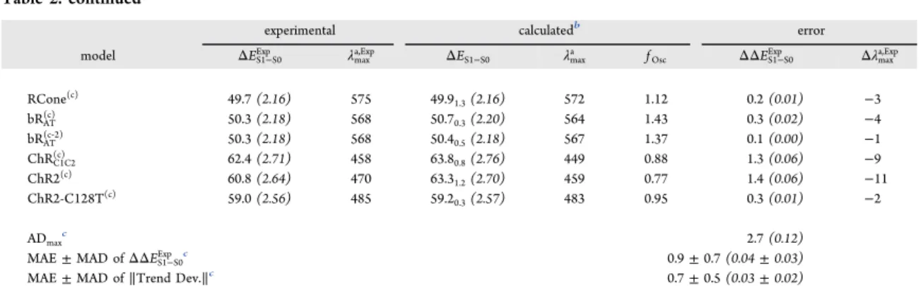
Table 2. continued

experimental calculatedb _error

model ΔES1−S0Exp λmaxa,Exp ΔES1−S0 λmaxa fOsc ΔΔES1−S0Exp Δλmaxa,Exp

RCone(c) _{49.7 (2.16) 575 49.9} 1.3(2.16) 572 1.12 0.2 (0.01) −3 bRAT(c) 50.3 (2.18) 568 50.70.3(2.20) 564 1.43 0.3 (0.02) −4 bRAT(c‑2) 50.3 (2.18) 568 50.40.5(2.18) 567 1.37 0.1 (0.00) −1 ChRC1C2(c) 62.4 (2.71) 458 63.80.8(2.76) 449 0.88 1.3 (0.06) −9 ChR2(c) _{60.8 (2.64) 470 63.3} 1.2(2.70) 459 0.77 1.4 (0.06) −11 ChR2-C128T(c) _{59.0 (2.56) 485 59.2} 0.3(2.57) 483 0.95 0.3 (0.01) −2 ADmaxc 2.7 (0.12)

MAE± MAD of ΔΔES1−S0Exp c 0.9± 0.7 (0.04 ± 0.03)

MAE± MAD of ∥Trend Dev.∥c _{0.7± 0.5 (0.03 ± 0.02)}

a_{Calculated using the a-ARMdefaultand the a-ARMcustomizedapproaches. Differences between calculated and experimental data (ΔΔES1−S0}Exp _,Δλmaxa,Exp₎ are also presented.bAverage value of 10 replicas, along with the corresponding standard deviation given as subindex.cFor BPR, bRAT, ChRC1C2, ChR2, ChR2-C128T, RCone, and KR2-2 a-ARMcustomizedare considered.dASRAT-2, ASR13C-1, KR2-1, and bRAT(c‑2)are excluded from the statistical analysis.

DOI:10.1021/acs.jctc.9b00061 J. Chem. Theory Comput. 2019, 15, 3134−3152 3145