ALGEBRAIC SURFACES WITH ISOLATED SINGULARITIES
E. FORTUNA, P. GIANNI, AND D. LUMINATI
Abstract. Given a real algebraic surface S inRP3, we propose a constructive procedure to
de-termine the topology of S and to compute non-trivial topological invariants for the pair (RP3, S)
under the hypothesis that the real singularities of S are isolated. In particular, starting from an implicit equation of the surface, we compute the number of connected components of S, their Euler characteristics and the weighted 2-adjacency graph of the surface.
1. Introduction
Given a real algebraic surface S in RP3 by means of an implicit equation, the problem of recognizing the topology of the surface can be addressed at two different levels: either considering
S only as an abstract topological space, or taking into account also its embedding in RP3 and looking at the topology of the pair (RP3, S).
When the surface S is non-singular, the possible topological models for the connected compo-nents of S are given by the topological classification theorem for surfaces. Thus, if S is implicitely defined by an equation of even degree, all its connected components are orientable topological 2-manifolds and hence homeomorphic to a sphere with g handles (i.e. to a sphere or, if g ≥ 1, to a torus with g holes); if the equation that defines S has an odd degree, then S contains exactly one non-orientable connected component homeomorphic to the connected sum of a projective plane and a sphere with g handles, while all the other components are orientable.
If we want to consider also how a surface is embedded in RP3, we say that two surfaces S, S0 are ambient-homeomorphic if there exists a homeomorphism ϕ : RP3→ RP3such that ϕ(S) = S0; in this case we also say that the pairs (RP3, S) and (RP3, S0) are homeomorphic. At present there is no classification of the pairs (RP3, S) up to homeomorphism even in the non-singular case and
deciding whether two pairs (RP3, S) and (RP3, S0) are homeomorphic is a very hard problem, also for simple classes of surfaces such as tori (with one hole). Hence a useful contribution in this direction is to be able to compute topological invariants of the pair (RP3, S).
A traditional approach to an algorithmical determination of the topology of a surface is via Cylindrical Algebraic Decomposition ([C] , see also [BPR]), which provides a cellular decomposition of the pair (RP3, S). Different approaches have been proposed by other authors, starting from
Gianni and Traverso ([GT]) who outlined a method based on the use of Morse theory; recently Mourrain and T´ecourt ([MT]) have proposed an algorithm that computes a simplicial complex isotopic to a given surface.
Developing the ideas in [GT], the papers [FGPT] and [FGL] give constructive answers to the problem of recognizing topologically a real algebraic non-singular surface proposing algorithms that compute the number of its connected components and the Euler characteristic of each of them, which determines them up to homeomorphism. In [FGLP] the non-singular surface is considered together with its embedding in RP3; the authors describe an algorithmical method to compute the
Date: July 15, 2005.
This research was partially supported by M.I.U.R. and by Eurocontract HPRN-CT-2001-00271.
“weighted adjacency graph” of the surface, which gives information both on the mutual disposition of the connected components and on their contractibility.
In this paper we address from a constructive point of view the same questions when the surface contains only isolated singularities. Our aim is to find a discrete set of data that are algorithmically computable, sufficient to determine the topology of the surface and that are non-trivial topological invariants for the pair (RP3, S).
For our approach the basic topological information is that in a small 3-dimensional ball D, centered at an isolated singular point, S ∩D is homeomorphic to the cone over the curve C obtained as the intersection of S with the boundary of the ball (see [M2]). Then, up to homeomorphism, the portion of S inside the ball can be seen as the space obtained taking the union of as many 2-dimensional disks as the connected components of C, choosing a point in each of these disks and collapsing these points to a single point. In this way we see the isolated singularity as the effect of two successive operations: first the glueing of a 2-cell (i.e. a subset homeomorphic to a closed 2-dimensional disk) along each connected component of C and then the collapsing of a set containing a point in each of the attached 2-cells.
Applying this procedure to all the singularities, we obtain a compact topological surface T without boundary such that S is homeomorphic to the topological quotient T /R where R is the equivalence relation that collapses suitable finite families of points of T . Thus our algorithm will determine topologically S by computing the Euler characteristics of the connected components of
T and the families of points that, through a collapsing process, produce the singularities of S.
Furthermore, after defining the weighted 2-adjacency graph of S, we show that it is a topological invariant of the pair (RP3, S) and we describe an algorithmical method to compute it.
This paper is a natural evolution of the articles [FGPT], [FGL] and [FGLP], which dealt with non-singular surfaces. Here we use the same basic ideas and techniques (use of a Morse projection, connecting paths, reduction to the affine case, etc.) but we insert them in a new procedure able to detect the presence of isolated singularities and to investigate their topological nature. Basically, while at a critical point most of the needed information is given by the index of that point, at an isolated singularity the necessary topological information will be obtained through the investigation of the curve where S intersects a small sphere centered at the singular point. Also to mantain the paper at a reasonable length, we have chosen to describe in detail only the topological results on which the algorithm bases its correctness and the organization of the main algorithm. As for the instrumental algorithmical techniques used as “black boxes”, we only recall their essential features and refer the reader to the papers previously mentioned for a detailed presentation.
The main definitions, the necessary theoretical background and the list D(S) of data invariant up to homeomorphism of the pair (RP3, S) to be computed are contained in Section 2. In order to
deal with isolated singularites we use a generalization of classical Morse theory to singular spaces, first introduced by Lazzeri ([L]), that we briefly recall in Section 3, where we prove also some related results necessary for the algorithm. In Section 4 we describe a constructive procedure to compute
D(S) when the surface is contained in an affine chart of RP3. This procedure can be applied if some preliminary tests have been positively passed, i.e. if the singularities of S are isolated and the working system of coordinates is a “good frame”; in Section 5 we present algorithms to perform both these tests and also some preliminary computations concerning the critical and singular points and some related data. When S is not affine, it is possible to construct a suitable compact algebraic surface bS in R3 and to recover D(S) from D( bS), which can be computed by
means of the affine-case algorithm. This reduction procedure and the general-case algorithm are presented in Section 6 which contains also some examples.
2. Some remarks on the topology of surfaces with isolated singularities Let S be the real projective algebraic surface in RP3 defined by the equation F (x, y, z, t) = 0, where F is a square-free homogeneous polynomial of degree d with real coefficients. A point P ∈ S is called a singular point of the surface if it annihilates all the first partial derivatives of F ; thus the set Sing S of the singular points of S is an algebraic set.
Recall that a point P ∈ S is called an isolated point of S if there exists an open neighborhood
U of P in RP3 such that S ∩ U = {P }; all isolated points of S are necessarily singular points. A
singular point P of S is called an isolated singular point if it is isolated in Sing S, i.e. if there exists an open neighborhood U of P such that (Sing S) ∩ U = {P }. We will consider only the case when each singular point of S is isolated in Sing S, so that Sing S is a discrete set containing finitely many points. Note that we make no assumption on the singular locus Sing SC of the complex
projective surface SCin CP3defined by the equation F = 0; since F is square-free, Sing SCcannot
have dimension 2, but it can be a complex curve.
If Q ∈ R3 and ² ∈ R, ² > 0, we will use the following notations to denote respectively the open
ball, the closed ball and the sphere of radius ² centered at Q: — B(Q, ²) = {X ∈ R3| d(X, Q) < ²}
— D(Q, ²) = {X ∈ R3 | d(X, Q) ≤ ²}
— S(Q, ²) = {X ∈ R3| d(X, Q) = ²},
where d(·, ·) denotes the Euclidean distance in R3. The previous notations make sense also for
points Q in RP3working in an affine chart U ' R3 containing Q.
If X is a topological space and Y a subspace, we will denote by G(X, Y ) the adjacency graph
of the pair (X, Y ), that is the graph whose vertices are the connected components of X \ Y and
where two distinct vertices Ω1, Ω2 are joined by an edge if and only if the topological closures of
Ω1 and Ω2 are not disjoint.
If Z is a topological space, the space Z × [0, 1]/Z × {1}, obtained by collapsing to a point the subspace Z × {1}, is called the cone over Z; we will denote it by Cone(Z). Conventionally the cone over the empty set consists of a point. If A ⊆ R3 and P is a point in R3, by cone over A with vertex P we will mean the union of all segments joining P with any point R ∈ A and we will
denote it by Cone(A, P ). Similarly by convention Cone(∅, P ) = {P }.
The following result, proved by Milnor also in the complex case, gives the important information that locally at an isolated singularity S is topologically a cone:
Theorem 2.1. ([M2], Proposition 2.10) Let Q be an isolated singular point of S. Then there
exists r > 0 such that for all positive ² ≤ r
i) C(Q, ²) := S ∩ S(Q, ²) is a non-singular curve (possibly empty) ii) S ∩ D(Q, ²) is homeomorphic to the cone over C(Q, ²).
Any r > 0 such that D(Q, r) \ {Q} contains no singular points of S and no critical points of the restriction to S of the function X → d(X, Q)2 satisfies the thesis of the previous theorem. For any ² ≤ r, we will call ² a Milnor radius at Q and S(Q, ²) a Milnor sphere at Q.
More precisely, using the Theorem of semialgebraic triviality for the function X → d(X, Q) and adapting suitably the proof of Theorem 9.3.6 in [BCR], we have:
Proposition 2.2. Let Q = (α, β, γ) be an isolated singular point of S. Let r be a Milnor radius
at Q both for the surface S and for the plane curve S ∩ {z = γ}. Then for all 0 < ² ≤ r there exists a homeomorphism φ : D(Q, ²) → D(Q, ²) such that:
(1) φ(S ∩ D(Q, ²)) = Cone(C(Q, ²), Q); (2) φ(D(Q, ²) ∩ {z = γ}) = D(Q, ²) ∩ {z = γ}; (3) φ(x) = x for all x ∈ S(Q, ²);
(4) φ(S(Q, ²0)) = S(Q, ²0) for all ²0 ≤ ². As an immediate consequence, one also has
Corollary 2.3. In the hypotheses of Proposition 2.2, we have
φ(S ∩ D(Q, ²) ∩ {z = γ}) = Cone(C(Q, ²) ∩ {z = γ}, Q).
Our strategy to study S will be based on the possibility of modifying S inside Milnor spheres centered at the singular points, getting a topological surface T ⊂ RP3 (i.e. a 2-dimensional topological manifold) from which we can obtain again S, except its isolated points if any, by means of a suitable quotient. We will construct T as an application of the following
Construction 2.4. Let X be a non-empty topological
1-dimen-ω2
ω1
ω3
Q
Figure 1. The construction de-scribed in 2.4
sional submanifold of a sphere S(Q, r). Let L1 be the adjacency
graph of the pair (S(Q, r), X); it is a tree having at least 2 ver-tices.
If L1has two vertices, then X is connected and we set W (X) = Cone(X, Q).
Otherwise denote by V1(L1) the set of the vertices of L1 of
valency 1. Any v ∈ V1(L1) is a connected component of S(Q, r) \ X homeomorphic to an open disk bounded by an oval ω(v) which
appears in L1 as the unique edge having v in its boundary. For i ∈ N denote by θi: S(Q, r) → S(Q,21ir) the function defined by θi(Y ) = 21i(Y − Q) + Q and let W1(X) = [ v∈V1(L1) µµ Cone(ω(v), Q) \ B(Q,1 2r) ¶ ∪ θ1(v) ¶ .
Then W1(X) is a union of disjoint 2-cells embedded in D(Q, r) and having as boundary the
curveSv∈V1(L1)ω(v) ⊆ X.
Let L2be the graph obtained from L1removing the vertices in V1(L1); it is the adjacency graph
of the curve X2= X \
S
v∈V1(L1)ω(v) of S(Q, r).
If L2has only one vertex (i.e. X2 is empty), we set W2(X) = ∅.
If L2has two vertices, we set W2(X) = Cone(X2, Q).
If L2has at least three vertices, we consider the set V1(L2) of its vertices of valency 1 and set W2(X) = [ v∈V1(L2) µµ Cone(ω(v), Q) \ B(Q, 1 22r) ¶ ∪ θ2(v) ¶ .
We iterate the constructive procedure until we get h ∈ N such that Lh has at most one vertex; then we let
W (X) = W1(X) ∪ . . . ∪ Wh−1(X). ¤ By construction we immediately get:
Lemma 2.5. Let X be a non-empty topological 1-dimensional submanifold of a sphere S(Q, r)
and denote by W (X) the subset of D(Q, r) described in Construction 2.4. Then W (X) is the union of finitely many disjoint 2-cells embedded in D(Q, r) such that
(1) the boundary of W (X) is the curve X, (2) W (X) ∩ S(Q, r) = X,
Assume at first, for simplicity, that Q is the only singular point of S. There are two possible situations:
– if Q is isolated in S, then S can be seen as the disjoint union of the point Q and the compact topological (not algebraic, in general) surface without boundary S \ {Q},
– if Q is not isolated in S and D(Q, ²) is a Milnor ball at Q, then S \ B(Q, ²) is a topological surface having as its boundary the non-empty curve C(Q, ²) = S ∩ S(Q, ²). Denote by T the topological surface without boundary embedded in RP3 which is the union of S \ B(Q, ²) and
the set W (C(Q, ²)) obtained applying Construction 2.4 to the curve C(Q, ²). Thus T is obtained from S removing S ∩ B(Q, ²) and attaching a 2-cell along each connected component of C(Q, ²). Choose a point in each of the attached 2-cells and denote by Z(Q) the set of these points. Then
S is homeomorphic to the topological quotient of T with respect to the equivalence relation that
collapses Z(Q) to a single point.
Coming back to the general case, henceforth we will denote by
• Q1, . . . , Qmthe singularities of the surface that are not isolated points in S, • R1, . . . , Rsthe isolated points in S.
Let ² be a small positive number such that D(Qi, ²) is a Milnor ball at Qi for i = 1, . . . , m and such that D(Qi, ²) ∩ D(Qj, ²) = ∅ whenever i 6= j. In particular Rh 6∈
Sm
i=1D(Qi, ²) for all h = 1, . . . , s.
If we remove from S the points R1, . . . , Rsand we apply Construction 2.4 to all the Milnor balls D(Qi, ²) (i.e. we attach a 2-cell along each connected component of S∩S(Qi, ²) for all i = 1, . . . , m), we get an embedded topological surface without boundary that we will denote by T henceforth. Again denote by Z(Qi) the set obtained choosing a point in each 2-cell attached to C(Qi, ²). If R is the equivalence relation on T that collapses to a point each of the sets Z(Q1), . . . , Z(Qm), then S is homeomorphic to the disjoint union of T /R and of the set {R1, . . . , Rs}.
The topological type of the space obtained by collapsing finitely many points in a compact con-nected surface does not depend on the choice of these points, but only on their number. Therefore, if T1, . . . , Trare the connected components of T , the topological type of T /R = (T1∪ . . . ∪ Tr)/R is completely determined by the topology of the Ti’s and by the number nij of points in Z(Qi) ∩ Tj for i = 1, . . . , m and j = 1, . . . , r.
If a compact connected surface is orientable, by the topological classification theorem for surfaces it is homeomorphic to the connected sum of a sphere and g tori, i.e. it is homeomorphic to a sphere with g handles. The number g, called genus, is a topological invariant that determines a compact connected orientable surface up to homeomorphism. We can equivalently determine any orientable connected surface by computing its Euler characteristic χ, since it turns out that χ = 2−2g (which in particular is always an even integer).
Again by the topological classification theorem, any compact connected non-orientable surface is homeomorphic to the connected sum of either a projective plane or a Klein bottle and a compact connected orientable surface of genus g; the Euler characteristic is then respectively either χ = 1−2g or χ = −2g, that is either odd or even. Note that a compact connected surface with an even Euler characteristic may be either orientable or non-orientable, so that in general the only knowledge of the characteristic is not sufficient to recognize topologically a compact connected surface, unless we know whether it is orientable or not. But it can be proved (see [V], 1.3.A) that the Euler characteristic of a non-orientable connected surface contained in RP3is necessarily odd. Hence the
knowledge of the Euler characteristics of the connected components of a compact surface embedded in RP3 completely determines the topological type of the surface.
Therefore, coming back to our situation, in order to determine the topological type of S, it will be sufficient to compute:
(1) the list χ(T ) = [χ1, . . . , χr] of the Euler characteristics of the connected components T1, . . . , Trof T ,
(2) m lists of non-negative integers, each having length r, say
l1= [n11, . . . , n1r], . . . , lm= [nm1, . . . , nmr] where nij= #(Z(Qi) ∩ Tj),
(3) the number s of isolated points in S.
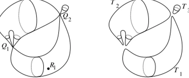
Example 2.6. The surface represented in Figure 2 has three isolated singularities Q1, Q2, R1and R1 is an isolated point, so that m = 2, s = 1. The topological surface T constructed as explained
above has three connected components T1, T2, T3 and all of them are spheres. The singularity Q1
can be obtained collapsing one point of T1 and two points of T2 to a single point; similarly Q2can
be obtained collapsing three points chosen respectively in T1, T2 and T3. Thus the topology of S
is determined by the following data: χ(T ) = [2, 2, 2], l1= [1, 2, 0], l2= [1, 1, 1], s = 1. ¤
Q1 R1 Q 2 T 3 T 1 T 2
Figure 2. A surface with three singular points (left-hand side) and the topological surface T associated to it (right-hand side).
So far our topological investigation has not taken into account the way in which the surface is embedded in RP3 and in particular it gives no information about the mutual disposition of the connected components of S and the connected components (or regions) of RP3\ S. In [FGLP] it
was shown how additional information can be obtained in the case of a non-singular surface by computing the adjacency graph of the surface, where two distinct vertices (i.e. regions of RP3\ S)
are joined by an edge if and only if their topological closures are not disjoint. When S is non-singular, two adjacent regions of RP3\ S share in their boundaries a connected component of S. Hence the edges of the adjacency graph of S are in 1-1 correspondence with the connected
components of the surface, with the only exception that, when S has an odd degree, the unique non-orientable component of S is not represented in the graph.
If S is singular, it may occur that the closures of two regions of the complement of S share only finitely many points; think for instance of the surface consisting of two spheres tangent at a common point. We will not consider two such regions ”really adjacent” and will be interested in the 2-adjacency graph G(S) whose vertices are the regions of RP3\ S, but in which two distinct
vertices are joined by an edge if and only if the closures of the two regions of RP3\ S meet in a
2-dimensional subset of S. Observe that
(1) the 2-adjacency graph G(S) just defined coincides with the ordinary adjacency graph when
S is non-singular,
(2) the graph G(S) is a topological invariant of the pair (RP3, S),
(3) the isolated points of S, if any, are not represented in G(S).
Unlike the non-singular case, there is not a bijective correspondence between the set of the edges of G(S) and the set of the connected components of the surface even if S has an even degree: for instance if S consists of two cones with the same vertex, S is connected but G(S) has two edges. Actually the next proposition shows that we recover similar properties if we consider the connected
components of S \ Sing S; the proof of this result, that we insert for completeness, may be omitted with no influence on the comprehension of the rest of the paper.
Proposition 2.7. Let S1, . . . , Sn be the connected components of S \ Sing S. Then
(1) If the degree of S is odd, then there exists a unique i such that, if we set Γ = Si, the set RP3\ Γ is connected, while for any j 6= i the set Sj disconnects RP3 into two connected regions.
(2) If the degree of S is even, for all j Sj disconnects RP3 into two connected regions. Proof. (1) The homology class [S] in H2(RP3, Z/2Z) is given by [S] =
Pn
i=1[Si]. If S has an odd degree, [S] is non-zero and hence there exists a component Si of S \ Sing S such that [Si] 6= 0.
Moreover for any j 6= i necessarily [Sj] = 0 because otherwise [Si] · [Sj] ∈ H1(RP3, Z/2Z) would
be non-trivial, which is impossible since Si∩ Sj⊂ Sing S consists of isolated points.
Let Γ = Si; we claim that RP3\ Γ is arcwise connected (and hence connected). Namely for each P, Q ∈ RP3\ Γ let α : [0, 1] → RP3 be a continuous path in RP3 joining P and Q. If α does not intersect Γ, the claim is proved; otherwise we can assume that α meets Γ in non-singular points of
S (i.e. lying in Γ) and transversally. Since Γ is homologically non-trivial, then Γ is non-orientable;
thus, if α(t0) ∈ Γ, there exists a loop γ in Γ passing through α(t0) and orientation-reversing for Γ.
If n(t) is a normal vector to Γ along γ , since RP3 is orientable, then n(1) = −n(0). It is therefore
possible to join α(t0−²) with α(t0+²) without intersecting Γ following the normal n(t). Repeating
this construction for each point where α meets Γ, eventually we get a path lying in RP3\ Γ and
joining P and Q.
We have only to prove that, for each Sj 6= Γ, RP3\ Sj is not connected. Otherwise, choosing a segment that meets transversally Sj in its medium point, and connecting the extremal points of this segment by means of a continuous path disjoint from Sj, we would find a closed curve δ that meets Sj only in one point. Then if we consider the homology classes [δ] ∈ H1(RP3, Z/2Z) and
[Sj] ∈ H2(RP3, Z/2Z), we would have [δ] · [Sj] = 1, in contradiction with the fact that [Sj] = 0. (2) When S is even-degree, we get the thesis arguing in a similar way. ¤ As a consequence of the previous result, there is a 1-1 correspondence between the closures of the connected components of S \ Sing S and the edges of G(S), except for odd-degree surfaces when the closure of the component Γ given by Proposition 2.7 is not represented in G(S).
Moreover, as a consequence of Lemma 2.5, it is not hard to see that
Proposition 2.8. The 2-adjacency graph G(S) is isomorphic to the adjacency graph G(T ). Apparently, not all information about the mutual position of couples of distinct regions of RP3\S
can be derived from the 2-adjacency graph G(S). For instance, if S consists of two spheres tangent at a point and each external to the other, the graph G(S) has 3 vertices and the two vertices corresponding to the interior parts of the two spheres are not joined by an edge, just as if the two spheres were disjoint. As a matter of fact, using the lists l1, . . . , lm relative to the singularities which are not isolated points in S, we can realize whether two regions not joined by an edge in
G(S) ' G(T ), and therefore not adjacent with respect to the surface T , meet at one or more points
of their boundaries after the collapsing process that yields S starting from T .
Recall that a subset A ⊂ RP3 is called contractible if any loop in A is contractible (i.e. homo-topically trivial) as a loop in RP3, non-contractible otherwise. Using this notion we can endow the vertices of G(T ) with weights by means of the function wT : {vertices of G(T )} → {c, nc} that marks each vertex of G(T ) (i.e. each region of RP3\ T ) as contractible or non-contractible.
Classical general results (see for instance [V]) ensure that the component Γ, if present, is always non-contractible, while the other components of T (that is the edges of G(T )) can be either contractible or non-contractible. Since it turns out that an edge of G(T ) is non-contractible if and
only if its two vertices are both non-contractible, the knowledge of the function wT is sufficient to know which components of T are contractible and which components are not. Let us recall that a contractible connected component W of T disconnects RP3 in two connected regions, only one of which is contractible and called the interior part of W . For such components it is possible to define a natural partial order relation: if Wiand Wjare two contractible connected components of T , we say that Wi< Wj if Wi is contained in the interior part of Wj. In [FGLP] it is shown how the graph G(T ) can be endowed with a set of roots r(T ) from which it is possible to reconstruct the previous partial order.
The triple (G(T ), wT, r(T )) will be called the weighted adjacency graph of T .
We can fix the same system of weights {c, nc} also on the vertices of the 2-adjacency graph
G(S) by means of wS : {vertices of G(S)} → {c, nc}. We will denote by Gnc(S) the subgraph of G(S) formed by the non-contractible vertices and by the edges having both vertices marked nc;
instead we will denote by Gc(S) the subgraph formed by all the contractible vertices, all the edges where at least one vertex is contractible and all the vertices of these edges. By means of arguments similar to those used in the proof of Proposition 2.7, one can see that, if S has an odd degree, all the regions of RP3\ S are contractible and hence Gnc(S) = ∅. Instead, when the degree of S is even, the closure Sjof each connected component of S \Sing S disconnects RP3into two connected regions and at least one of them is non-contractible (possibly both, as in the case of a one-sheeted hyperboloid); in particular Gnc(S) is not empty.
In the singular case, it is no longer true that the weights on the two vertices of an edge are sufficient to determine the contractibility of the edge. For instance, if S is a cone, G(S) has two vertices, one marked c, the other nc and still the only edge of G(S) (i.e. the cone itself) is non-contractible. However the knowledge of the weights on the vertices of G(S) is sufficient to define a partial order relation in the set of the closures of the connected components of S \ Sing S as precised in the following:
Definition 2.9. Let Si and Sj be distinct connected components of S \ Sing S. We say that Si is inside Sj if the following two conditions hold:
(1) Sj disconnects RP3 into two regions and one of these is contractible, (2) Si is contained in the contractible component of RP3\ Sj.
All the information necessary to know the previous partial order among the sets Si can be obtained by choosing some roots in the 2-adjacency graph G(S). The way in which this can be done depends on the degree of S.
If S has an even degree, Gnc(S) is connected and each connected component of Gc(S) is a tree that contains exactly one vertex weighted nc: we choose these vertices as a set of roots of G(S). In this way the order induced on each connected component of Gc(S) by the only root contained in it coincides with the partial order described in Definition 2.9.
If S has an odd degree, Gnc(S) is empty; however we are able to choose a root in G(S) also in this case: we will call root of G(S) the unique region of RP3\ S which is adherent to the connected
component Γ given by Proposition 2.7.
Note that, while for even-degree surfaces the information about which vertices are the roots of G(S) is obtained from the weights, for odd-degree surfaces this notion is independent of the weights on G(S) because in this case each vertex is marked c. However this piece of information is quite important since sometimes it is the only one that allows to realize that two pairs (RP3, S)
and (RP3, S0) are not homeomorphic: if, for instance, S consists of a projective plane and two topological spheres, only the knowledge of the root allows to recognize whether the two spheres are mutually external or one of them encircles the other one.
If r(S) denotes the set of roots of S defined as above, the triple (G(S), wS, r(S)) will be called the weighted 2-adjacency graph of S. With the previous definitions it is easy to see that
Proposition 2.10. (i) The weighted 2-adjacency graph of S is an invariant of the pair (RP3, S) up to homeomorphism.
(ii) The weighted 2-adjacency graph of S is isomorphic to the weighted adjacency graph of T .
The isolated points of S do not appear at all in G(S). While their number is sufficient for the topological characterization of S, in order to take into account the embedding of S in RP3we need to know in which regions of the complement they lie. For that it will be sufficient to compute a list q = [q1, . . . , qs] where qi is the region of RP3\ T containing the i-th isolated point Ri.
We will collect all the mentioned data concerning the surface in a single list of data
D(S) = [χ(T ), G(T ), wT, r(T ), l1, . . . , lm, q]. By the previous considerations we have that
(1) D(S) is an invariant up to homeomorphism of the pair (RP3, S),
(2) D(S) completely determines the topological type of S,
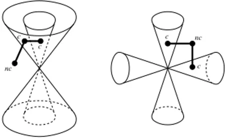
(3) though not sufficient to determine the pair (RP3, S), the set D(S) gives useful
informa-tion on the surface up to ambient-homeomorphism. For instance the surfaces S and S0 represented in Figure 3 are homeomorphic but the pairs (RP3, S) and (RP3, S0) are not homeomorphic since the weighted adjacency graphs of T and T0 are not isomorphic.
nc c c nc c c
Figure 3. Two surfaces that are homeomorphic, but not ambient-homeomorphic.
The next sections will be devoted to show that all the data in D(S) can be computed starting from an equation of S, even if T is not algebraic.
3. Passing through a critical or a singular point
In this section we start to describe our general strategy to compute the topology of a real algebraic surface S having only isolated singularities and we present the mathematical theoretical results on which the algorithm bases its correctness. In the present section we assume that S is contained in an affine chart of RP3 (as we will see, this is the basic case to be dealt with), so that we can see it as a compact affine surface in R3 defined by a polynomial equation f (x, y, z) = 0.
When S is non-singular it is possible to set up an algorithmical procedure to study S topo-logically using results from classical Morse theory. We refer to [FGPT], [FGL] and [FGLP] for a detailed description of such an algorithm; we recall here only its essential features as an help for the reader and for a later generalization.
Denote by p : S → R the projection defined by p(x, y, z) = z. A point P ∈ S is a critical point for p if it is non-singular but it annihilates the first partial derivatives fxand fy; in this case p(P ) is called a critical value. Recall (see [M2] Corollary 2.8) that p can have at most finitely many critical values.
A critical point P for p is called non-degenerate if it does not annihilate the determinant of the Hessian matrix
µ
fxx fxy fxy fyy
; by index of a non-degenerate critical point P one means the number of negative eigenvalues of the Hessian matrix of p at P with respect to local coordinates; it can be computed from fz and the Hessian matrix of f . If S is non-singular the projection p is a Morse function if any critical point for p is non-degenerate.
For each a ∈ R we will denote by Ca the level curve p−1(a) = S ∩ {z = a} and by Sa the level surface p−1([−N, a]) = S ∩ {z ≤ a} having C
a as its boundary.
In the non-singular case the basic idea to compute the topology of S is to find N > 0 such that S ⊂ R2× [−N, N ], to subdivide R2× [−N, N ] as the union of finitely many adjacent strips
R2× [a, b] each containing only one critical point and to compute iteratively the topology of S b from the one of Sa by computing the Euler characteristics of all the connected components of the level surface. Recall that χ is a homotopic invariant, i.e. if X and Y are homotopically equivalent, then χ(X) = χ(Y ); hence a crucial tool to get information on the topology of Sb is given by the following result from classical Morse theory:
Theorem 3.1. (cfr. [M1], Theorem 3.1 and Theorem 3.2) Assume that [a, b] is an interval such
that a and b are regular values for the projection p.
(1) If the strip R2× (a, b) contains no critical point for p, then S
a is homeomorphic to Sb (and furthermore Sa is a deformation retract of Sb).
(2) If R2× (a, b) contains only one point Q which is a non-degenerate critical point for p of index k = 0, 1, 2, then Sb is homotopically equivalent to the space obtained from Sa by attaching a k-cell.
This theorem, using only the index information, allows to compute how the global Euler charac-teristic of the level surface changes when passing through a (non-degenerate) critical point of index
k, since it increases by (−1)k. However it is not sufficient to reconstruct properly the topological type of Sb, i.e. its connected components and their Euler characteristics. To do that, it is also necessary to know how a k-cell is attached to the boundary of Sa. For instance in the case of a 1-cell it is important to detect whether it is attached to one or two components of Sa. This can be done by means of a more accurate analysis of the surface in the strip R2× [a, b] based on the
topological study of the level curves Ca and Cb and on a careful lifting procedure, for instance to recognize whether an oval of Ca and an oval of Cb bound the same connected component of S ∩ (R2× [a, b]) or not.
This is why in the iterative step the main algorithm makes use of two special-purpose procedures already described in previous papers in the literature. The first one is used to study the shape of
a level curve in correspondence of a regular value for p; in this case the level curve is an affine
non-singular compact algebraic curve, so that all its connected components are ovals. Recall that an oval is called empty if it contains no other oval in its interior part, and a list [ω1, . . . , ωt] of ovals of a curve is called a nest of depth t if ω1is empty, ωi is contained in the interior part of ωi+1 for all i = 1, . . . t − 1 (and any other oval containing ωi contains also ωi+1) and ωtis not contained in the interior part of any oval of the curve.
In correspondence of a regular value, say for instance b, the pair ({z = b}, Cb) is determined up to homeomorphism by the list of its nests or equivalently by the adjacency graph of the pair ({z = b}, Cb), that we simply denote by G(Cb). The first “black box” algorithmically computes G(Cb) starting from the equation f (x, y, b) = 0 of Cb; several authors have proposed algorithms to do that (see for instance [GT], [CGT], [AMcC], [R], [CGVR]) and one can use whichever of them. It is also possible (see for instance [FGPT]), by means of standard techniques, to enrich the curve-algorithm with special functions; namely, for a non-singular curve C,
– the function f indRegion, given a point P ∈ R2\ C, returns the connected component (or region) f indRegion(P ) of R2\ C containing P ,
– the function f indOvals, given a point P ∈ R2, returns the list of the ovals of C containing P
ordered by inclusion starting from the innermost oval,
– the function f indP oint, given an oval ω of C, returns a point lying inside ω, more precisely a point R such that ω is the first oval of the sequence f indOvals(R).
The second special-purpose procedure in the iterative step is needed to lift and relate information from the level {z = a} to the level {z = b}. This will be done by means of connecting paths: if
P ∈ {a ≤ z ≤ b} \ S, we will denote by pathU p(P, b) (resp. pathDown(P, a)) the final point α(1)
of a continuous path α : [0, 1] → {a ≤ z ≤ b} not intersecting S and such that α(0) = P and
α(1) ∈ {z = b} (resp. α(1) ∈ {z = a}).
In [FGLP] one can find a proof of the following
Proposition 3.2. Assume that a and b are regular values for p and that R2× (a, b) contains at most a point Q which is a non-degenerate critical point for p. Let Ω be a region of (R2×[a, b])\Sand let P be any point of Ω. Then
(1) if Q is critical of index 0 or of index 1, it is possible to construct an upward connecting
path from P to pathU p(P, b) contained in Ω
(2) if Q is critical of index 2 or of index 1, it is possible to construct a downward connecting
path from P to pathDown(P, a) contained in Ω
The previous results, in particular Theorem 3.1, are important but not sufficient to handle the situation we are dealing with in this paper, i.e. when S contains isolated real singular points. However it is possible to get information about how the level surface changes when passing through an isolated singularity by using a generalization of Morse theory for singular spaces, first outlined by Lazzeri ([L]) and then furtherly developed by [P] and [GMcP]. First of all it is necessary to generalize the notion of Morse function:
Definition 3.3. (1) A singular point Q = (α, β, γ) ∈ S is called non-degenerate with respect
to the projection p if there exists no sequence {Qn} of non-singular points of the surface converging to Q such that the horizontal plane {z = γ} passing through Q is the limit (in the Grassmannian of the 2-planes of R3) of the tangent planes T
Qn(S) to S at Qn. (2) The projection p is a Morse function on S if all the (smooth) critical points and all the
real singular points of S are non-degenerate.
From the theory presented in [L] one can obtain the following result that generalizes Theorem 3.1 to the singular case:
Theorem 3.4. ([L]) Let Q = (α, β, γ) be an isolated singular point for the surface S, which is
non-degenerate w.r.t. the projection p(x, y, z) = z. Assume that a < γ < b and that the strip
R2× [a, b] contains neither critical points for p nor singular points of S except Q. Then there exists r > 0 and a continuous function η : R+→ R+ such that
(1) for 0 < ² ≤ r and for 0 < η ≤ η(²) the plane set S ∩ {z = γ − η} ∩ D(Q, ²) is a smooth
compact curve (possibly with boundary) whose diffeomorphism class does not depend on η, so that we can denote it simply by M (Q),
(2) Sγ is a deformation retract of Sb,
(3) if K is a deformation retract of M (Q), then Sb is homotopically equivalent to Sγ−η ∪ Cone(K, Q),
(4) if ϕ : Sγ−η → Sa is a homeomorphism, then Sb is homotopically equivalent to the space obtained attaching to Sa the set Cone(K) along K0= ϕ(K).
Thus, if M (Q) is simply an oval, the cone over it is topologically a disk so that passing through
Q we have the attachment of a 2-cell to the boundary of Sa. Since an arc of curve is homotopically equivalent to a point, if M (Q) consists of l arcs then we have the attachment of the cone over l points. In general if M (Q) consists of h ovals and l arcs, Sbis obtained attaching to the boundary of Sa the cone over h ovals and l points.
Note that the previous description of the homotopy type of Sb with respect to Sa holds also when Q is a non-degenerate critical point of index k, and in fact the only one contained in the strip R2× (a, b). Namely, if Q has index 2 then M (Q) is an oval and the cone over it is a 2-cell;
if Q has index 1 then M (Q) is the union of 2 arcs, so that we can take as K a couple of points and the cone over them is topologically a 1-cell; if Q has index 0, then M (Q) is empty and the cone over it is a point, i.e. a 0-cell. In other words Theorem 3.4 generalizes Theorem 3.1 replacing the index of the critical point with the plane curve M (Q) as a source of information sufficient to describe the level surface Sb up to homotopy equivalence when passing through the point Q.
For computational reasons we will furtherly modify our source of topological information, prov-ing that we can get a topological model of M (Q) inspectprov-ing the intersection of S with a sphere
S(Q, ²) centered at a singular point Q = (α, β, γ) provided that ² is a Milnor radius both for S and
for the curve S ∩ {z = γ} at Q. This topological equivalence will be computationally relevant be-cause it will allow us to perform our computations on the fixed sphere S(Q, ²) without the problem of computing an η(²) sufficiently small so that the curve S ∩ {z = γ − η} ∩ D(Q, ²) is guaranteed to be topologically (and diffeomorphically) stable for all positive η < η(²).
For the rest of the section we will assume that
• ² is a Milnor radius both for S and for the curve S ∩ {z = γ} at Q = (α, β, γ),
• D(Q, ²) is contained in the interior part of a strip R2× [a, b] which contains no critical
points for the projection p and no singular points of S except Q.
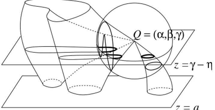
We will see that the asymptotic behaviour, for η → 0, of the horizontal plane section S ∩ {z =
γ − η} near the singular point Q is strictly related to the position of the connected components of
the curve C(Q, ²) = S ∩ S(Q, ²) with respect to the circle S(Q, ²) ∩ {z = γ}. It will therefore be useful to introduce the following terminology:
Definition 3.5. If Q = (α, β, γ), a subset X of S(Q, ²) is called (1) of type (+) if X ⊆ {z > γ}
(2) of type (−) if X ⊆ {z < γ} (3) of type (+−) if X ∩ {z = γ} 6= ∅.
Though C(Q, ²) is not a plane curve, we will call its connected components ovals. First of all let us prove that the type of an oval of C(Q, ²) does not change if we reduce the sphere radius: Proposition 3.6. Let ω be an oval of C(Q, ²). Denote by Y the connected component of (S ∩
D(Q, ²)) \ {Q} containing ω. For ²0≤ ², let ω(²0) = Y ∩ S(Q, ²0). Then, for all ²0≤ ² we have: (1) If ω is an oval of type (+) (resp. (−)), then ω(²0) is an oval of type (+) (resp. (−)). (2) If ω is an oval of type (+−), then ω(²0) is an oval of type (+−) and ω(²0)∩{z = γ} contains
as many points as ω ∩ {z = γ}.
Proof. Let Y = Y ∪ {Q}. By Proposition 2.2 and Corollary 2.3, there exists a homeomorphism φ : D(Q, ²) → D(Q, ²) such that φ(S ∩ D(Q, ²) ∩ {z = γ}) = Cone(C(Q, ²) ∩ {z = γ}, Q)) and φ(Y ) = Cone(ω, Q). In particular Y is topologically a disk. Then Y ∩ {z = γ} is homeomorphic
to the cone Cone(ω ∩ {z = γ}, Q).
If ω is of type (+) (resp. (−)), then ω ∩ {z = γ} = ∅ and hence Cone(ω ∩ {z = γ}, Q) = {Q}. Then Y ∩ {z = γ} = {Q} and Y ∩ {z = γ} = ∅. It follows that Y ⊆ {z > γ} (resp. {z < γ}) so that ω(²0) is of type (+) (resp. (−).
In the case ω is of type (+−) the thesis follows in the same way, observing that if ω∩{z = γ} consists of k points, then Y ∩ {z = γ} is homeomorphic to the cone over k points and so ω(²0) ∩ {z = γ} is homeomorphic to Cone(ω ∩ {z = γ}, Q) ∩ S(Q, ²0) hence it consists of exactly k points. ¤ Later on, it will be important also the following result on the positions of the ovals of C(Q, ²): Lemma 3.7. Let ω be an oval of C(Q, ²). Then ω is transversal to {z = γ}.
Proof. By contradiction suppose that ω is tangent to {z = γ} at a point P . Since ² is a Milnor
radius for S ∩ {z = γ}, then the curve S ∩ {z = γ} is transversal to the sphere S(Q, ²); hence the tangent line to that curve at P is transversal to S(Q, ²). Since the tangent line to ω at P is tangent to the sphere S(Q, ²), the tangent plane to S at P is generated by two transversal horizontal lines. Hence P is a critical point for the projection p, which is a contradiction. ¤
Q
= (α,β,γ)
z =
z = a
γ − η
Figure 4. Sections of a surface with a Milnor sphere centered at a singular point Q and with a horizontal plane {z = γ − η} passing below the singularity.
We are now ready to compare the local behaviour near a singular point of horizontal sections of S with the intersection of S with a Milnor sphere:
Proposition 3.8. Let ω and Y be as in Proposition 3.6. Then there exists η0> 0 such that for all positive η ≤ η0 we have:
(1) if ω is an oval of type (−), then Y ∩ {z = γ − η} consists of exactly one oval;
(2) if ω is an oval of type (+−), and more precisely ω ∩ {z ≤ γ} is the union of k arcs, then
Y ∩ {z = γ − η} is the union of k arcs too.
Proof. (1) Let η0 > 0 be such that ω ⊂ {z < γ − η0}. By connectivity, for any η ≤ η0 the set Y ∩ {z = γ − η} is not empty. Since ω ∩ {z = γ − η} = ∅ and the plane {z = γ − η} is transversal
to Y , then Y ∩ {z = γ − η} is a non-singular curve without boundary, i.e. consisting only of ovals. We have to prove that it consists of just one oval.
Suppose by contradiction that there exists η0≤ η
0such that Y ∩{z = γ−η0} contains at least two
ovals. Then, since there are no critical points in the strip {γ − η0≤ z < γ}, the same is true for all
sections Y ∩{z = γ−η} with η ≤ η0; morover, for all η1< η2≤ η0the set Y ∩{γ−η2≤ z ≤ γ−η1} is
a disconnected cylinder. This means that Y ∩ {γ − η2≤ z < γ} is disconnected: otherwise if τ were
a path in Y ∩ {γ − η2≤ z < γ} joining two points in two different components of Y ∩ {z = γ − η2},
it would exist a positive η < η2 such that τ ⊆ Y ∩ {γ − η2≤ z ≤ γ − η} contradicting the fact that
this set is a disconnected cylinder.
If Y = Y ∪ {Q}, the sets Uη= Y ∩ {γ − η ≤ z ≤ γ}, with 0 < η < η0, are a fundamental system
of neighborhoods of Q in Y , i.e. for any ρ > 0 there exists η such that Uη ⊆ B(Q, ρ). Otherwise there exist ρ and a sequence of points Pn ∈ Y ∩ {γ −n1 ≤ z ≤ γ} such that Pn6∈ B(Q, ρ). Since Y
is compact, we can assume that {Pn} converges to a point P ∈ Y ∩ {z = γ} = {Q}, contradicting the fact that Pn6∈ B(Q, ρ).
The sets Uη are connected, because any point P ∈ Uη can be joined to Q by a path in Uη. Namely, if ρ < η, let η0be such that U
η0 ⊆ B(Q, ρ) ∩ Y ⊆ Uη. Then, since Y ∩ {γ − η ≤ z ≤ γ − η0} is a cylinder, P can be joined to a point in Uη0 and hence also to Q because B(Q, ρ) ∩ Y is a cone. We have so found a fundamental system of neighborhoods of Q in Y that are disconnected removing the point Q, in contradiction with the fact that Y is homeomorphic to a disk.
Observe in particular that Uη is topologically a disk.
(2) Since by Lemma 3.7 ω is transversal to {z = γ}, there exists η0> 0 such that ω ∩{z ≤ γ −η}
is the union of k arcs for all η ≤ η0. Furthermore, for η ≤ η0 by a transversality argument Y ∩ {z = γ − η} is a smooth curve with a boundary equal to ω ∩ {z = γ − η} and hence it contains
exactly k arcs .
We have to prove that this curve cannot contain any oval. Suppose that there exists η0 such that Y ∩ {z = γ − η0} contains an oval σ. Since Y is homeomorphic to a disk, then σ disconnects Y . Let Y0 the connected component of Y \ σ not containing ω. It is clear that Y0∩ S(Q, ²) = ∅.
Let m = minY0z and M = maxY0z. Since the function p(x, y, z) = z cannot be constant on Y0, then M 6= m, and since z is constant on the boundary of Y0 then at least one of them must be achieved in an interior point R of Y0.
If Q 6∈ Y0, such a point R should be a smooth point of S and thus a critical point for the function p on S, while no such point exists in the strip we are working in.
Suppose instead that Q ∈ Y0. If the maximum M were achieved in a point different from Q, we would have a contradiction as before. So we can suppose that Y0\ {Q} ⊆ {z < γ}. The set Y0 is open in Y , hence for ²0small enough D(Q, ²0)∩Y ⊆ Y0. Then D(Q, ²0)∩Y = D(Q, ²0)∩Y0and thus S(Q, ²0) ∩ Y = S(Q, ²0) ∩ Y0. Since Y0\ {Q} ⊆ {z < γ}, we have S(Q, ²0) ∩ Y ⊆ S(Q, ²0) ∩ {z < γ} which means that ω(²0) = Y ∩ S(Q, ²0) should be an oval of type (−), contradicting Proposition
3.6. ¤
As a consequence of Theorem 3.4 and Proposition 3.8, we can describe the change of the topology of Sbwith respect to Sain terms of the ovals of C(Q, ²): passing through Q we have the attachment of the cone over h ovals and l points, where h is the number of ovals of C(Q, ²) of type (−) and l is the number of distinct arcs obtained intersecting all the ovals of C(Q, ²) of type (+−) with the negative halfsphere S(Q, ²) ∩ {z ≤ γ}.
Recall however that our true goal is not reconstructing globally the topology of Sb from that of Sa, but the topology of Tb from that of Ta and not globally but component by component. There are at least two remarkable differences: firstly S ∩ D(Q, ²) is connected while T ∩ D(Q, ²) may be non-connected; secondly, while Sγ is homotopically equivalent to Sb, in general Tγ is not homotopically equivalent to Tb because of the contributions due to the ovals of type (+).
In order to detect the independent contributions to the topology of the various connected compo-nents of Tbwhen passing through Q, a more careful analysis of the situation is needed. Henceforth we will use the following
Notation 3.9. If ω is an oval of C(Q, ²), we will denote by T (ω) the connected component of (T ∩ {a ≤ z ≤ b}) \ B(Q, ²) containing ω in its boundary.
Again a fundamental tool will be the possibility of constructing connecting paths starting from points on the Milnor sphere, which is easily achieved as a corollary of Proposition 3.2:
Corollary 3.10. Assume that a and b are regular values for p and that R2× (a, b) contains no critical point for p and a unique singular point Q = (α, β, γ). Let D(Q, ²) be a Milnor ball contained in R2× (a, b) and let Ω be a region of (R2× [a, b]) \ (S ∪ D(Q, ²)). Then
(1) if P ∈ S(Q, ²) ∩ {z > γ} ∩ Ω, then it is possible to construct an upward connecting path
from P to pathU p(P, b) contained in Ω
(2) if P ∈ S(Q, ²) ∩ {z < γ} ∩ Ω, then it is possible to construct a downward connecting path
from P to pathDown(P, a) contained in Ω.
Similarly to the non-singular case, by computing finitely many connecting paths starting from points on the Milnor sphere, it will be possible to detect which ovals of Ca∪ Cb are contained in T (ω) and thus to lift correctly all the data.
Let us conclude the section with some results that give information about T (ω) ∩ (Ca ∪ Cb) according to the type of ω.
Proposition 3.11. Let ω be an oval of C(Q, ²). If ω is of type (−) (resp.(+)), then T (ω)∩{z = a}
(resp. T (ω) ∩ {z = b}) consists of a single oval ω0, the boundary of T (ω) is ω ∪ ω0 and T (ω) is homeomorphic to a cylinder.
Proof. Assume for instance that ω is of type (−) and denote by Y the connected component of
(S ∩ D(Q, ²)) \ {Q} containing ω. Let η0 be such that ω ⊂ {z < γ − η0}; by Proposition 3.8 Y ∩ {z = γ − η0} is an oval, say λ. The set S ∩ {a ≤ z ≤ γ − η0} is a cylinder; let Λ be its connected
component containing λ. Hence Λ ∩ {z = a} consists of a single oval ω0.
The set Y = Y ∪ {Q} is topologically a disk; in the proof of Proposition 3.8 we saw that the sets Uη = Y ∩ {γ − η ≤ z ≤ γ}, with 0 < η ≤ η0, form a fundamental system of connected
neighborhoods of Q in Y and that Uη is topologically a disk. Then Y \ Uη0 is a connected cylinder
containing λ and ω and contained in S ∩ {a ≤ z ≤ γ − η0}; in particular Y \ Uη0 ⊆ Λ and hence ω ⊂ Λ.
Furthermore, since Λ ∪ Y = Λ ∪ Uη0 and Uη0 is a disk with boundary λ, then Λ ∪ Y is a disk
with boundary ω0, the set Λ \ Y = (Λ ∪ Y ) \ Y is a connected cylinder with boundary ω ∪ ω0 and Λ \ Y is a closed connected cylinder with boundary ω ∪ ω0.
In order to get the thesis, it suffices to prove that Λ \ Y = T (ω).
First of all we claim that Λ∩D(Q, ²) is connected. Namely otherwise, since Λ∩{z = γ −η0} = λ,
there exists a connected component W of Λ ∩ D(Q, ²) not containing λ, i.e. W ∩ {z = γ − η0} = ∅.
Then the boundary of W is contained in S(Q, ²) and there exists a point P ∈ W ∩ B(Q, ²) critical for the distance function d(Q, X)2, contradicting the fact that B(Q, ²) is a Milnor ball for S.
Therefore Λ∩D(Q, ²) is a connected set containing ω, hence Λ∩D(Q, ²) ⊆ Y , which implies that Λ \ Y ∩ B(Q, ²) = ∅. Thus Λ \ Y is a connected surface contained in S ∩ {a ≤ z ≤ b} \ B(Q, ²) (and hence in T ∩ {a ≤ z ≤ b} \ B(Q, ²)) with boundary ω ∪ ω0. Recall that if N ⊆ M are two surfaces such that N is connected and the boundary of N is contained in the boundary of M , then N is a connected component of M . Then Λ \ Y is the connected component of T ∩ {a ≤ z ≤ b} \ B(Q, ²)
containing ω, i.e. Λ \ Y = T (ω), which concludes the proof. ¤
This latter Proposition, together with the previous results, is sufficient to determine the contri-bution to the topology of Tb given by the ovals of type (−) or of type (+):
• if ω is of type (+), attaching a 2-cell along ω to S \ B(Q, ²), there appears in Tb a new connected component homeomorphic to a disk and with boundary ω0⊂ C
b; it is therefore topologically equivalent to passing through a critical point of index 0;
• if ω is of type (−), the attachment of a 2-cell along ω is topologically equivalent to the
attachment of a 2-cell along an oval ω0 of C
a (and hence equivalent to passing through a critical point of index 2); thus it contributes increasing by 1 the Euler characteristic of the connected component of Tb containing ω. Note that such a component may intersect S(Q, ²) also in other ovals of type (−) or (+−), thus its topology passing from level a to
As for the ovals of type (+−), again using Theorem 3.4 and Proposition 3.8 we get some information about the effect of the attachment of a 2-cell along each of them. Namely we already know that, if ω is an oval of type (+−) that intersects k arcs on the negative halfsphere, the attachment of a 2-cell along ω is homotopically equivalent to the attachment of the cone over k points to the boundary of Ta(ω), where Ta(ω) denotes the union of the connected components of Ta containing in their boundaries the ovals of T (ω) ∩ Ca. Hence all these components of Ta glue together into a component of Tbcontaining ω and the Euler characteristic of this latter component is increased by 1−k with respect to the sum of the Euler characteristics of the connected components of Ta(ω).
More precisely, if W is a connected component of Tb such that W ∩ S(Q, ²) consists of ovals of type (−) and/or (+−), then χ(W ) is equal to the sum of the Euler characteristics of the connected components of W ∩ {z ≤ a} increased by 1 for each oval of type (−) and increased by 1 − ki for each oval ωi of type (+−) that contains ki negative arcs.
Of course now the situation is more complicated because the boundary of T (ω), apart from
ω, can contain several ovals of Ca and several ovals of Cb that we need to detect by means of connecting paths. This can be done applying the following result to the connected components in which a region of type (+−) of S(Q, ²) \ S is split by {z = γ}:
Proposition 3.12. Let A be a region of S(Q, ²) \ (S ∪ {z = γ}). Then:
(1) if A is contained in {z > γ} and Ω is a region of {γ < z ≤ b} \ (S ∪ D(Q, ²)) containing
A in its boundary, then Ω ∩ {z = b} is non-empty and connected,
(2) if A is contained in {z < γ} and Ω is a region of {a ≤ z < γ} \ (S ∪ D(Q, ²)) containing
A in its boundary, then Ω ∩ {z = a} is non-empty and connected.
Proof. Consider for instance case (1). By Corollary 3.10 we have that Ω ∩ {z = b} is non-empty.
If P1, P2∈ Ω ∩ {z = b}, there exist two paths joining respectively P1 and P2 to a point R ∈ A and
contained in Ω. Hence we have a path σ joining P1 with P2 and contained in {γ < z ≤ b} \ S.
Then there exists γ0> γ such that σ is contained in {γ0≤ z ≤ b} \ S. Since the interval [γ0, b] does not contain critical values, also the connected components of {γ0≤ z ≤ b} \ S are cylinders, hence
σ can be deformed to a path in {z = b} \ Cb joining P1 and P2. ¤
4. The compact affine case
In this section we describe a constructive procedure to compute the list of data D(S) = [χ(T ), G(T ), wT, r(T ), l1, . . . , lm, q] when the real algebraic surface S defined in RP3 by the ho-mogeneous equation F (x, y, z, t) = 0 and having only isolated singularities does not intersect in real points the plane “at infinity” {t = 0} ⊂ RP3. In this case S is contained in the affine chart {[x, y, z, t] ∈ RP3 | t 6= 0} ' R3 and can be studied working in affine coordinates; namely f (x, y, z) = F (x, y, z, 1) = 0 is an affine equation for S.
The projection p : S → R, p(x, y, z) = z can have at most finitely many critical values and under our hypotheses S can have at most finitely many (real) singular points. Up to a generic linear change of coordinates we can assume (see [P]) that our system of coordinates (x, y, z) is a
good frame, that is
i) the projection p is a Morse function (i.e. any critical point for p and any singular point of
S is non-degenerate)
ii) if P1and P2 are either singular or critical and P16= P2, then p(P1) 6= p(P2).
In this section we assume to have already checked that S has only isolated singularities and that the given system of coordinates (x, y, z) is a good frame; also we assume to have already computed the critical points and their indexes, the singularities and a Milnor radius at each of them (more precisely, for each singular point Q, an r which is a Milnor radius at Q both for the surface and
for the plane curve obtained intersecting S with the horizontal plane through Q). In Section 5 we will see how these preliminary tests and computations can be performed.
Let [−N, N ] be an interval containing all the critical values of p and all the images through p of the singular points of S (that, for simplicity, we will call singular values). We can subdivide it as [−N, N ] = [−N = a0, a1] ∪ [a1, a2] ∪ . . . ∪ [au, au+1 = N ] so that each ai is neither critical nor singular and each interval (ai, ai+1) contains only one critical value or one singular value.
Since the singular points are only finitely many, we can assume that ² ∈ Q is positive and so small that
– D(Qi, ²) is a Milnor ball at the singular point Qi, for any i = 1, . . . , m, both for S and for the curve S ∩ {z = γi} where {z = γi} is the horizontal plane passing through Qi,
– D(Rj, ²) is a Milnor ball for S at the isolated point Rj for any j = 1, . . . , s, – D(Qi, ²) ∩ {z = ah} = ∅ ∀i = 1, . . . , m and ∀h = 0, . . . , u + 1
– D(Rj, ²) ∩ {z = ah} = ∅ ∀j = 1, . . . , s and ∀h = 0, . . . , u + 1.
Thus each Milnor ball of radius ² centered at a singular point is contained in a single open strip R2× (a
h, ah+1) and does not intersect any level plane {z = ah}.
As usual, denote by T the embedded topological surface without boundary obtained from S removing the points R1, . . . , Rs and applying Construction 2.4 to all the Milnor disks D(Qi, ²); then, for each h = 0, . . . , u + 1, we have that
(1) Cah= S ∩ {z = ah} = T ∩ {z = ah}
(2) Tah = T ∩{z ≤ ah} is a topological surface with boundary Cah obtained from Sahremoving the points Ri that lie in {z < ah} and applying Construction 2.4 to the Milnor disks D(Qi, ²) contained in {z < ah}.
Thus each Sah is homeomorphic to the disjoint union of the isolated points Rjlying in {z < ah} and the quotient space Tah/Rh, where Rh is the restriction to Tah of the equivalence relation R introduced in Section 2. Hence at each level we can get topological information on Sah studying the topological level surface Tah.
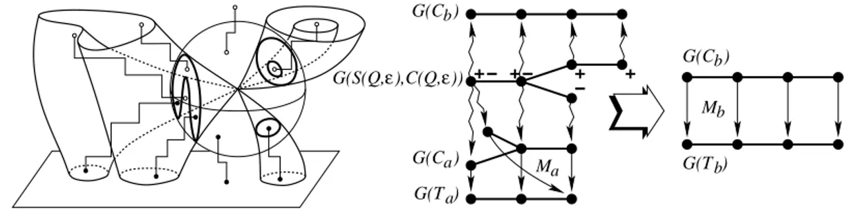
Our constructive procedure to compute the list of data D(S) will be based on the following Theorem 4.1. (Iterative Step) Let [a, b] be an interval such that a and b are regular values and R2× (a, b) contains only one point Q which is either critical for p or singular for S. Then it is possible to compute
Output(Sb) = {G(Cb), χ(Tb), G(Tb), Mb, l1(Tb), . . . , lm(Tb), q(Tb)} starting from Output(Sa), where
i) Cb= S ∩ {z = b} = T ∩ {z = b} and G(Cb) is the adjacency graph of the pair ({z = b}, Cb), ii) Tb = T ∩ {z ≤ b} and χ(Tb) is the list of the Euler characteristics of the connected
components of Tb
iii) G(Tb) is the adjacency graph of the pair ({z ≤ b}, Tb),
iv) Mb: G(Cb) → G(Tb) is the graph morphism that associates to each vertex v of G(Cb) the vertex of G(Tb) representing the region of {z ≤ b} \ Tb having in its boundary the region of {z = b} \ Cb represented by v
v) li(Tb) = [ni1, . . . , nir] where nijis the number of points of Z(Qi) lying in the j-th component of Tb (note that r depends on b)
vi) q(Tb) is a list of length s where the i-th element is the region of {z ≤ b} \ Tb containing the i-th isolated point Ri if Ri ∈ {z ≤ b}, it is 0 otherwise.
Before proving this theorem, let us show that it easily allows to achieve our main goal: Corollary 4.2. There is an algorithmical procedure to compute D(S).
Proof. At at the initial step both C−N and T−N are empty, so that G(C−N) and G(T−N) consist of a single vertex. The lists l1, . . . , lm, q are initialized as the zero lists; during the iterative procedure only the lists li(Tb) concerning the singular points Qilying in {z < b} are non-zero.
Since TN = T , the data χ(T ), G(T ), l1, . . . , lm, q contained in the list D(S) will be obtained after applying iteratively Theorem 4.1 to the intervals [−N, a1], . . . , [au, N ]. At the end of the iterative procedure, the only data that we still need to compute to get D(S) are the function wT and the roots r(T ). In the affine case this is straightforward: since T is contained in the affine chart {t 6= 0} of RP3, all its components are contractible and all the regions of RP3\T are contractible except the
only one external to all the components of T . The algorithm easily recognizes this external region as the only vertex in G(T−N); we choose it as the only root of G(T ), mark it as non-contractible
and mark as contractible all other vertices in G(T ). ¤
Example 4.3. Consider again the surface of Example 2.6 represented in the left-hand side of Figure 2. Focusing for instance our attention on the reconstruction of χ(T ), l1, l2, q, we want to
see how these data (already announced in Example 2.6) are obtained at the end of the iterative procedure in the strips represented in Figure 5.
Q1 R1 a6 a a 5 4 a3 2 a a1 a0 a7 a8 Q 2
Figure 5. Level planes and strips for the iterative reconstruction process. Output(Sa1): Sa1 = Ta1 is a disk, hence χ(Ta1) = [1], l1= [0], l2= [0], q = [0].
Output(Sa2): we pass through a point which is isolated in S, hence χ(Ta2) = [1], l1 = [0], l2 =
[0], q = [1] (where we label 1 the region of {z ≤ a2} \ Ta2 containing the isolated point).
Output(Sa3): passing through a critical point of index 1 influences only the Euler characteristic
and we get χ(Ta3) = [0], l1= [0], l2= [0], q = [1].
Output(Sa4): the strip {a3≤ z ≤ a4} contains the singular point Q1; Ta4 is the disjoint union of
three disks and, apart from the isolated point R1, Sa4 is homeomophic to Ta4/R where R collapses
to one point a set of three points lying respectively in the three connected components of Ta4.
Hence χ(Ta4) = [1, 1, 1], l1= [1, 1, 1], l2= [0, 0, 0], q = [1].
Output(Sa5): two connected components of Ta4 glue together, so that Ta5 is the union of two
disks and consequently the length of the lists l1 and l2 becomes 2. We get χ(Ta5) = [1, 1], l1 =
[1, 2], l2= [0, 0], q = [1].
Output(Sa6): we pass through the singular point Q2; Ta6 is the union of a sphere and two disks; Q2 is obtained collapsing one point in that sphere with two points chosen respectively in the two
disks so that χ(Ta6) = [2, 1, 1], l1= [1, 2, 0], l2= [1, 1, 1], q = [1].
Output(Sa7): only the Euler characteristics are modified passing through the critical point of index
2 contained in this strip and we get χ(Ta7) = [2, 1, 2], l1= [1, 2, 0], l2= [1, 1, 1], q = [1]. Output(Sa8): passing through the last critical point of index 2 we get the final expected data
χ(Ta8) = χ(T ) = [2, 2, 2], l1= [1, 2, 0], l2= [1, 1, 1], q = [1]. ¤
The remaining part of the section will be devoted to the Proof of Theorem 4.1, i.e. to see how it is possible to compute Output(Sb) from Output(Sa) in the Iterative Step.
![Figure 5. Level planes and strips for the iterative reconstruction process. Output(S a 1 ): S a 1 = T a 1 is a disk, hence χ(T a 1 ) = [1], l 1 = [0], l 2 = [0], q = [0].](https://thumb-eu.123doks.com/thumbv2/123dokorg/2948827.23334/18.918.359.545.488.649/figure-level-planes-strips-iterative-reconstruction-process-output.webp)