Chapter 7
Front-Wheel Drive Car Simulations
In this chapter we analyze the behavior of a front wheel drive car, characterized by the same parameters as the vehicle we referred in the previous chapter.
7.1
High Speed
In this first simulation we illustrate the vehicle behavior in case the driver imposes a too
wide steer angle, considering the car speed. Initially the car is driving at 65 m
s and the
steer angle follows a step function which final value is 0.75 deg.
480 500 520 540 560 580 600 620 20 30 40 50 60 70 80 distance (m) distance (m) NO control ESP Redistribution Redistribution & ESP
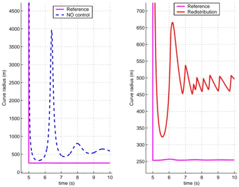
car which does not use these systems. This fact is also confirmed analyzing the graphs representing the trend of the “R” distance (fig.7.2 and fig.7.3).
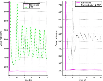
The radius of corner followed by the car which is not provided with any Yaw Control System presents an oscillating trend, with a very high peak after 6.4 s. Although both the speed and the steer angle are bigger than in the “Simulation A” (par. 6.1) this car does not spin around and it has a motion closer to the reference than the corresponding rear-wheel drive car. For this reason we can say that a front-wheel drive car is usually “more stable” than a rear-wheel drive car. However it does not mean that improvement of the vehicle behavior is not possible. We can notice that the curves referring to the other vehicles have still an oscillating performance but the stability systems manage to bring the peak values to a much lower level. Furthermore the cars provided with the “Haldex” coupling or with the combined system (central coupling and ESP) drive along narrower corners almost during the whole simulation. To use just the ESP causes a less regular behavior but the average bend radius is lower than the one followed by the non controlled vehicle, as we can see in fig.7.1.
5 6 7 8 9 10 0 500 1000 1500 2000 2500 3000 3500 4000 4500 time (s) Curve radius (m) 5 6 7 8 9 10 250 300 350 400 450 500 550 600 650 700 time (s) Curve radius (m) Reference NO control Reference Redistribution
5 6 7 8 9 10 300 400 500 600 700 800 900 1000 time (s) Curve radius (m) 5 6 7 8 9 10 250 300 350 400 450 500 550 600 650 700 time (s) Curve radius (m) Reference ESP Reference Redistribution & ESP
Figure 7.3: Comparison among the “R” distances
7.2
External Disturbance
In this simulation we want to present the effects of our stability systems in case the front outer wheel suddenly looses grip. This fact creates understeer, and it can be considered for example representative of a car which drives on an icy spot. The initial speed is 35 m s and the steer angle function is a step which final value is 1.5 deg. To model the loss of grip we considered the parameters a2 and b2 (see respectively (2.20) and (2.23)) depending on time, as shown in fig.7.4. Analyzing the trajectories (fig.7.5) we can observe that using independently the ESP system or the redistribution of torque the vehicle does not drive along a curve very different from the one followed by car non provided with any systems.
Only combining the ESP with the central coupling we manage to bring the trajectory closer to that the car would drive along if there was no external disturbance. Although we can have this performance improvement, the undisturbed trajectory remains quite distant from the other ones. We wandered why correcting an oversteering behavior is easier than to correct understeer. In fact, except for very extreme conditions (usually due to an exter-nal intervention and not due just to the vehicle intrinsic behavior) it is possible to correct satisfactorily an oversteering motion controlling the central coupling. This phenomenon is
0 5 10 15 500 600 700 800 900 1000 1100 1200 time (s) a2 0 5 10 15 600 700 800 900 1000 1100 1200 1300 time (s) b2 a2 data1data1 b2
Figure 7.4: Friction coefficients
260 270 280 290 300 310 320 330 340 350 360 100 150 200 250 distance (m) distance (m) NO control ESP
Redistribution & ESP Redistribution NO loss of grip
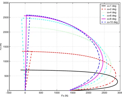
−5000 0 500 1000 1500 2000 2500 3000 500 1000 1500 2000 2500 3000 Fx (N) Fy (N) α=1 deg α=2 deg α=4 deg α=6 deg α=8 deg α=10 deg
Figure 7.6: Forces transferred by the tyre in combined slip conditions
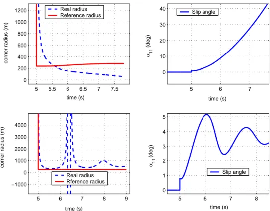
we can notice that usually the slip angles are inclined to increase, instead the understeer causes a decrease of the slip angles (for example see fig.7.7).
The curves represented in fig.7.6 make us understand the fact that the wider is the slip angle (α) the more the longitudinal force influences the lateral force. For example considering the curve regarding α = 1 deg and the curve concerning α = 10 deg, we want
to observe that a longitudinal force of 2000 N decreases Fy at α = 1 deg about 75 N. The
Fy at 10 deg slip angle instead has a decrease close to 800 N, therefore the longitudinal force has an almost 10 times stronger effect. Consequently the yaw moment produced by the coupling intervention will be much bigger in this last case, rather than in the first one. This is the reason why the redistribution of torque is much more effective when the vehicle is oversteering, rather than when it is understeering.
This argumentation is valid to explain the outcomes of our simulations but to under-stand better the effects of our Active Yaw Control during a real emergency condition we should take into account the driver’ s reactions. For example in a situation like that il-lustrated in this paragraph, when the car starts deviating from the expected trajectory, a common driver would increase the steer angle, then the front slip angles increase as well.
5 6 7 8 0 1 2 3 4 5 time (s) α11 (deg) 5 6 7 8 9 −1000 0 1000 2000 3000 4000 time (s) corner radius (m) 5 5.5 6 6.5 7 7.5 0 200 400 600 800 1000 1200 time (s) corner radius (m) 5 6 7 0 10 20 30 40 time (s) α11 (deg) Real radius
Reference radius Slip angle
Slip angle Real radius
Rference radius
Figure 7.7: Typical “R” distances and slip angles in oversteering (top) and understeering (bottom) conditions.
7.3
Avoidance Manoeuvre A
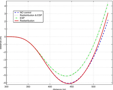
We simulated a front-wheel drive car making the same manoeuvre as the rear-wheel drive car described in the par.6.4 (“Avoidance manoeuvre”). Also in this case the front-wheel drive car demonstrated to be easier to drive than the corresponding rear-wheel drive vehicle. As shown in fig.7.8, the vehicle drives along a not very wide trajectory even if no stability control is used. Moreover to supply the vehicle with an “Haldex” coupling is almost useless. Providing or not a vehicle with the central coupling, the followed trajectories are practically the same, both using just the redistribution of torque system and combining the central coupling with an ESP. On the contrary the ESP is able to improve the car behavior, even if the maximum distance between the two trajectories is lower than 1 m. We want also to remark that the |β| angles are quite small during the whole simulation.
300 350 400 450 500 −6 −5 −4 −3 −2 −1 0 1 2 3 4 distance (m) distance (m) NO control Redistribution & ESP ESP
Redistribution
Figure 7.8: Trajectories followed by the cars
7.4
Avoidance Manoeuvre B
To create a more critical manoeuvre we increased the initial speed to 70 m
s and we changed
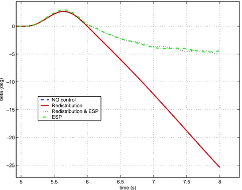
the curve representing the steer angle (fig.7.9). It has bigger amplitude and it has a double frequency than the function used in the previous simulations (fig.6.27). Comparing the trajectories we can understand that also in this simulation the effects of the redistribution of torque are almost negligible. Analyzing just fig.7.10 we could think that in this case the Yaw Control Systems affect negatively the vehicle behavior. In fact using the ESP (it is the only stability control system which causes a substantial effect) the manoeuvre takes a wider space. However if we analyze better the vehicle motion observing the body slip angle (fig.7.11) we realize that also in this case our systems work properly.
The non controlled car presents a β angle decreasing more and more, and after less than two seconds it exceeds the imposed threshold (-10 deg). On the contrary the cars provided with the ESP behave such a way that the body slip angle is never lower than -5 deg during the whole simulation. This fact can be considered a very good improvement in the car behavior even if the vehicle moves a little bit more on the right (approximatively
0 1 2 3 4 5 6 7 8 9 10 −1 −0.8 −0.6 −0.4 −0.2 0 0.2 0.4 0.6 0.8 1 time (s)
steering angle (deg)
Steering angle
Figure 7.9: Steer angle function
380 400 420 440 460 480 500 520 540 560 −3 −2 −1 0 1 2 3 4 5 6 7 distance (m) distance (m) NO control Redistribution & ESP ESP
Redistribution
5 5.5 6 6.5 7 7.5 8 −25 −20 −15 −10 −5 0 time (s)
beta (deg) NO control
Redistribution Redistribution & ESP ESP