Ansys model 3

(1)

Chapter

3

Ansys model

Contents

3.1 Introduction . . . 50 3.2 Combustion Chamber Outer Casing, CCOC . . . 50 3.2.1 System, CCOC plus probe . . . 56 3.2.2 First three families of nodal circles of nodal diameters with

refined model . . . 58 3.3 Comparison of the CCOC with Rolls Royce model . . . 58 3.3.1 Rolls Royce model . . . 58 3.3.2 Plot Nodal diameter-Frequency for the unclamped model,

free-free . . . 58 3.3.3 Plot Nodal diameter-Frequency for the clamped models . 59 3.4 Harmonic analysis, rigid brackets for the probe . . . 64 3.4.1 Modal analysis of the probe . . . 64 3.4.2 Modal analysis of the system, CCOC plus probe . . . 65 3.4.3 Comparison of a simulated mounted probe on the CCOC

and the simulated test configuration . . . 65 3.5 Harmonic analysis, rigid brackets and forces alongz . . 72 3.6 CCOC clamped by simple supports . . . 78

3.6.1 Harmonic analysis of the CCOC clamped by simple sup-ports, single force along z as harmonic excitation . . . 79 3.6.2 Harmonic analysis of the CCOC clamped by simple

sup-ports, displacements along z on one face as harmonic exci-tation . . . 79 3.7 Discussion . . . 87

(2)

3.1 Introduction

The chapter focus on the dynamic behaviour of an aircraft casing and a probe, its general accessory. In the first part a modal analysis is carried out for the aircraft casing and for the probe. The next step is a harmonic analysis for the probe in two different configurations as in the previous chapter. A real configuration, when the probe is attached at the aircraft casing, and a test room configuration, when the probe is installed on a shaker as a different input. Here, 6 DOFs for element is used leading a more accurate model compare to the previous chapter where only 1 DOF for element was considered. The Matlab scripts used in this chapter are reported in Appendix B.1.

3.2 Combustion Chamber Outer Casing, CCOC

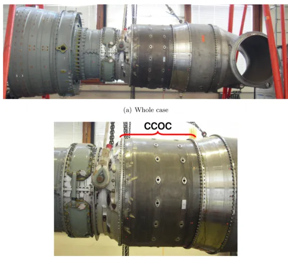
In this section, a part of an aircraft engine, Combustion Chamber Outer Casing (CCOC), is studied. The simplest model can be constructed from a cylinder with two small flanges on the end faces. This simple model was chosen because of low computational cost. The geometric dimensions for this model, see Table 3.1, were taken from Pegasus, an aircraft casing present in the laboratory of the Department of Mechanical Engineering at Imperial College London, see Figure 3.1. The material properties shown in Table 3.2 were taken from model used by Rolls Royce.

For the modal and the harmonic analysis, which were carried out with Ansys,

Table 3.1: Geometric dimensions of the CCOC

Radius 0.4 m

Length 0.5 m

Thickness 0.005 m

Table 3.2: Material properties of the CCOC

Density 8023 kg/m3

Poisson’s ratio 0.3

Young’s modulus 185 GP a

(3)

3.2. COMBUSTION CHAMBER OUTER CASING, CCOC

(a) Whole case

(b) Combustion Chamber Outer Casing

Figure 3.1: Pegasus

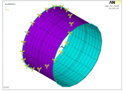
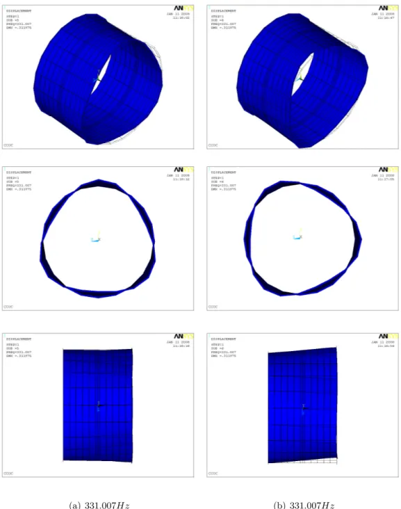
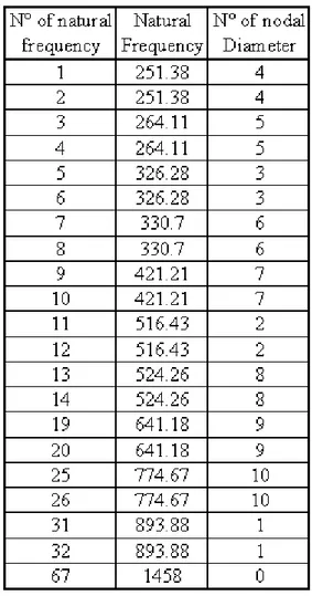
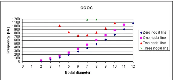
the circumference, and all DOFs on one face of the cylinder were constrained while those on the other side were free. This is shown as a cantilever in Figure 3.2. Natural frequencies and the plot Nodal diameter-Frequency for this model corresponding to the modes with zero nodal circles, are presented in Figure 3.3. It worth noting that for each number of nodal diameters there are two coincidental natural frequencies. This is because of the axi-symmetry of the system, see for an example Figure 3.4. It will be shown later that for a non axi-symmetric model those two natural frequencies are not coincidental. This is valid with the exception of two cases where for each nodal diameter only one natural frequency exist:

(4)

Figure 3.2: Shell model of the CCOC with constraint, rough mesh

For this problem the element size was large to show this property of the cylinder with few nodal diameters. The large element size leads the mesh to be unconvergent, which produces natural frequencies of higher value than the real well meshed model.

(5)

(6)

(a) 331.007Hz (b) 331.007Hz

Figure 3.4: 5th and 6th mode shape of the CCOC clamped one side, third nodal diameter and zero nodal circles

(7)

Figure 3.5: Zero nodal diameter and zero nodal circles

(8)

3.2.1 System, CCOC plus probe

A modal analysis of the system composed of the CCOC with a generic probe was conducted.

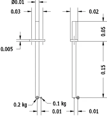
The probe is made of a frame which supports a beam, Beam4 was used as the element. At the end of the beam, two masses were joined by a rigid bracket (infinite stiffness) to make the probe asymmetric. M ass21 and CERIG were used as mass and rigid elements respectively. The geometric dimensions of the probe are shown in Figure 3.7, and the material properties in Table 3.3. The probe is fixed on

Figure 3.7: Drawing of the probe

Table 3.3: Material properties of the probe

Density 7800 kg/m3

Poisson’s ratio 0.3

Young’s modulus 211 GP a

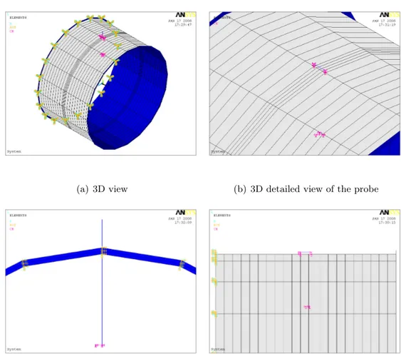
the mid-length of the cylinder, CCOC, by two rigid clamp screws set on the same generatrix of the cylinder, see Figure 3.8. CE, pink symbols in the figure, is the Ansys_{command which defines a constraint equation relating degrees of freedom. In}

(9)

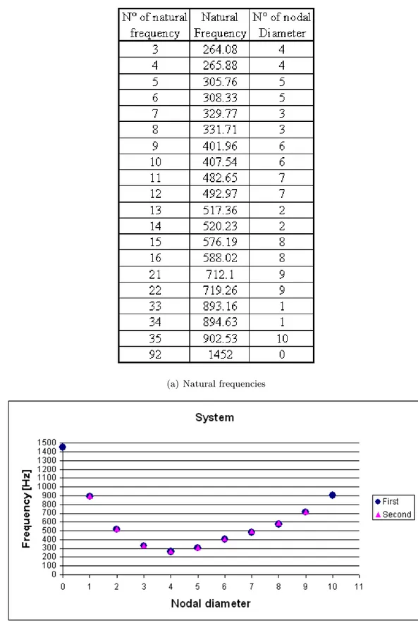
this case, CE was used to fix the probe at the engine and the masses at the probe. The natural frequency plot for this system corresponding to the zero nodal circles

(a) 3D view (b) 3D detailed view of the probe

(c) Front detailed view of the probe (d) Side detailed view of the probe

Figure 3.8: System, CCOC plus probe

is shown in Figure 3.9. Contrary to the plot of the CCOC, see Figure 3.3, where the model was axi-symmetric, for this configuration the system is not axi-symmetric because of the probe. Therefore the two natural frequencies corresponding to the same nodal diameter are separated, as shown in Figure 3.9. This is more evident from the table in Figure 3.9(a), than from the plot because for this case these natural frequencies are not so far apart.

(10)

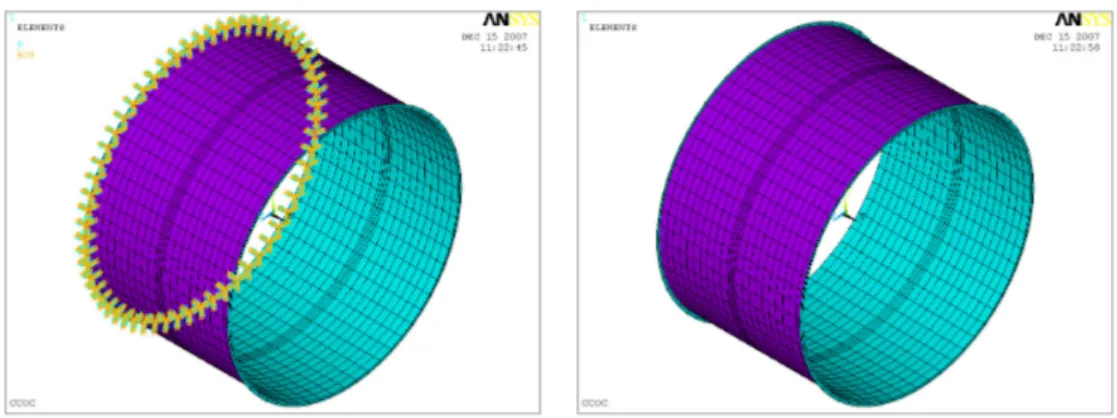
3.2.2 First three families of nodal circles of nodal diameters with refined model

On the previous model of the CCOC better mesh was assigned, which is fit for purpose, see Figure 3.11. The first three nodal circles families of the nodal diameters were found by modal analysis, the results are shown in Figure 3.12. The comparison of the natural frequencies of this model and the previous one, shows a rough mesh produces an apparent stiffness of the structure.

3.3 Comparison of the CCOC with Rolls Royce model

In this section, the dynamic behaviour of the model of CCOC well meshed with ≈ 10000 DOFs, see Figure 3.11 is compared to a more detailed Rolls Royce model of a similar structure, ≈ 130000 DOFs. Pictures, natural frequencies and responses of the model used by Rolls Royce cannot be reproduced here for copyright reasons.

3.3.1 Rolls Royce model

The Rolls Royce model is composed of a cylinder made out of shell elements and a large number of pipes attached at the case with CP elements which defines a set of coupled degrees of freedom. This model has a high computational cost and a modal analysis carried out of it produces too many natural frequencies, which are mainly due to the pipes. Clearly, this is beyond of the scope of the current research, which aims is to compare the previous model of the CCOC to a similar structure. Therefore only the case of the Rolls Royce model without the pipes and the CP elements is studied. It should be noted that if the CP elements were kept on the case without pipes, the natural frequencies of the case would be higher than the natural frequencies of the case without CP because they give a local stiffness, but clearly it does not make sense to keep the CP without the pipes.

3.3.2 Plot Nodal diameter-Frequency for the unclamped model, free-free

The CCOC and Rolls Royce models, without the pipes and the CP elements, were studied free-free, the first six natural frequencies are zero because they correspond with rigid body modes. It is usual to study a structure as free-free because it is the preferable way to carry out the test to validate the F E model. The related plot Nodal diameter-Frequency for the CCOC is shown in Figure 3.13. The comparison of

(11)

3.3. COMPARISON OF THE CCOC WITH ROLLS ROYCE MODEL

this plot and the plot relative to the Rolls Royce model showed that those models are similar around the low natural frequencies.

3.3.3 Plot Nodal diameter-Frequency for the clamped models

To see the opposite extreme of the clamping range, both ends were clamped. In this case, there were no rigid body modes. The related plot Nodal diameter-Frequency for the CCOC is shown in Figure 3.14, as in the previous case where these models were similar around the low natural frequencies. For this study the free-free and clamped configuration, are not ideal. The first method is not accurate because in general the structures are constrained or connected to each other, which influence the dynamic behaviour. The second way is also inaccurate, because even if there are frame or other structures attached at the part being analysed, such constraints are not infinitely rigid as represented here. The truth is in the middle of these two cases and it is hard to find the appropriate boundary conditions.

(12)

(a) Natural frequencies

(b) Nodal diameter-Frequency, first and second mean natural frequency for nodal diameter

Figure 3.9: Natural frequencies concerned modes shape of CCOC, System constrained on one side

(13)

(a) 329.768Hz (b) 331.71Hz

Figure 3.10: Zero nodal circles and third nodal diameter for the System

(a) With constraint (b) Without constraint

(14)

(a) Natural frequencies for the first nodal circles family

(b) Plot (Nodal diameter-Frequency) for the first three nodal circles families

(15)

Figure 3.13: CCOC unclamped, free-free

(16)

3.4 Harmonic analysis, rigid brackets for the probe

All the rotations and the translations on one side of the CCOC were constrained while on the other side a harmonic force of 10000 N , is distributed around four points, was applied along y from 0 to 500[Hz], as shown in Figure 3.15. A damping ratio of 2% was used.

(a) Draft

Figure 3.15: System used for the harmonic analysis, force along y

3.4.1 Modal analysis of the probe

For the modal analysis of the probe, shown in Figure 3.7, the probe was assumed to be fixed by rigid brackets on a rigid frame. The natural frequencies, ωi, in the

range 0 to 500[Hz] are:

ω1= 81.15 Hz ω2 = 82.5 Hz

(17)

3.4. HARMONIC ANALYSIS, RIGID BRACKETS FOR THE PROBE

Figure 3.16: First mode shape of the probe clamped by rigid brackets

Figure 3.17: Second mode shape of the probe clamped by rigid brackets

3.4.2 Modal analysis of the system, CCOC plus probe

Modal analysis was carried out for the system, the natural frequency results are shown in Figure 3.18. The first two natural frequencies are mainly due to the probe and the higher ones are due to the CCOC.

3.4.3 Comparison of a simulated mounted probe on the CCOC and the simulated test configuration

The real configuration is the system composed of the probe on the CCOC fixed by rigid brackets. The test configuration is composed of the probe clamped at the shaker at two mounting points. All elements have six DOFs, three translations (ux,

(18)

Figure 3.18: Natural frequencies of CCOC, probe and system

The same two locations were monitored for both configurations to allow a comparison: • monitoring point, P u, is the tip of the probe inside the CCOC. It is used to

compare the behaviour of the probe in those two different configurations • mounting point, M u1, is the first bracket where the probe is fixed at the

CCOC or at the shaker. The response of this point is measured on the real configuration and afterwards is applied by the shaker to the probe in the test configuration.

Vertical direction of monitoring pointP uy, vertical direction of the mount-ing point, M uy1

The vertical displacement, uy, was considered as the direction of interest, see Figure 3.19(a). The results of Figure 3.19(b) show that the gap between those two configurations is small and negligible. The maximum gap is around the natural frequencies of the CCOC.

Axial direction of monitoring and mounting point, P ux and M ux1

Here, the axial displacement, ux, was considered as the direction of interest, see Figure 3.20(a). As the shaker is only able to apply displacement orthogonal to the

(19)

(a) Draft

(b) Comparison P uy applying M uy1 by the shaker

Figure 3.19: Real configuration and test configuration, translation along y for both points: monitoring and mounting. Uy is vertical displacement with respect to the

(20)

plane where it is fixed, the probe must be rotated by 90◦ _{with respect to the real}

configuration that is being simulated. The results of Figure 3.20(b) show under testing for the probe around the natural frequencies of the CCOC.

Axial direction of monitoring point P ux, vertical direction of the mount-ing point, M uy1

The axial displacement for the monitoring point, P ux, and the vertical displace-ment, M uy1, for the mounting point, were considered, as shown in Figure 3.21(a).

In contrast to the previous cases, where the gap was significant only around the natural frequencies of the CCOC, in this case, the gap is also high around the natural frequencies of the probe, as shown in Figure 3.21.

Axial direction of monitoring and mounting point, P ux and M ux1,

maxi-mum value of M ux1 is used as input for the shaker

The axial displacement for the monitoring point, P ux, was considered. The maximum value of the axial displacement M ux1 was used as input for the shaker in

the frequency range 0 to 500[Hz], see Figure 3.22(a). The results of Figure 3.22(b), show that there is a large amount of over testing for the probe around the low natural frequencies while there is under testing for the high natural frequencies. At the high frequencies, the vibration environment is mainly due to the CCOC, which acts as a cantilever with a prevalence of vibration along y.

Displacement control on the shaker, axial direction of monitoring and mounting point

The logic used is shown in Figure 3.4.3. The output from the real configuration, probe on the CCOC, is used as the target point for the probe on the shaker where xs is found as input to have the same response as the target point. Figure 3.24(a)

shows that the axial displacement of the target point, P ux, has the same response for the probe on the CCOC, system, as for the probe on the shaker. Figure 3.24(b) shows how much extra excitation is required for the probe on the shaker to have the same displacement in axial direction leading to over testing for the mounting points in this direction.

(21)

(a) Draft

(b) Comparison P ux applying M ux1 by the shaker

Figure 3.20: Real configuration and test configuration, translation along x for both points: monitoring and mounting. Ux is axial displacement with respect to the

(22)

(a) Draft

(b) Comparison P ux applying M uy1by the shaker

Figure 3.21: Real configuration and test configuration, translation along x and y for the monitoring and mounting points respectively

(23)

(a) Draft

(b) Comparison P ux applying M ux1 by the shaker

Figure 3.22: Real configuration and test configuration, translation along x for both points: monitoring and mounting. The maximum value of M ux1 is used as input for

(24)

Figure 3.23: Draft of the displacement control on the shaker

3.5 Harmonic analysis, rigid brackets and forces along z

A harmonic force of 10000 N , distributed around four points, was applied along z on the face of the CCOC model. The displacement along z of the tip of the probe, P uz, was taken as a comparison point for the probe on the CCOC and for the probe on the shaker and the response in z of the first mounting point M uz1 was used as

input for the shaker, see Figure 3.25. The comparison between the two monitoring points P uz shows under testing for the probe over the whole frequency range, see Figure 3.26. As shows in Figure 3.27, the displacement of the tip of the probe is a combination of the translational displacements and the rotations of the mounting points. The rotations, which have a large influence on P uz, cannot be given as input for the probe by the shaker. This explains the large amount of under testing to which the probe is subjected. It should be noted how the probe reacts to the mounting point response on the shaker. Figure 3.28 plots the monitoring response P uz for the probe on the shaker, and the mounting point response M uz1 used as input for

the shaker. P uz is higher compared to M uz1 at the low frequencies because of the

(25)

3.5. HARMONIC ANALYSIS, RIGID BRACKETS AND FORCES ALONG Z

(a) Target point response of displacement control on the shaker, P ux

(26)

(a) Draft

(27)

Figure 3.26: Real configuration and test configuration, translation along z for both points: monitoring and mounting

(28)

also Figure 3.29.

Figure 3.28: Comparison between the input for the shaker, mounting point response from the system M uz1, and output from the probe on the shaker, P uz1

(29)

Figure 3.29: Deformed and underformed shape of the probe on the shaker, 75 Hz and , 283 Hz

(30)

3.6 CCOC clamped by simple supports

As discussed in the previous sections, it is not easy to find the suitable boundary condition for the CCOC. A right model to simulate the behaviour of the CCOC could be a complete model of engine, but obviously that has a high computational cost. Rolls Royce suggests that the following boundary conditions for the CCOC are the closest to the real model:

• all rotational DOFs are unrestrained and all translational DOFs are fixed on one face

• all rotational DOFs are unrestrained and all axial translation DOFs, in x, are also unrestrained on the other face

(a) Front view (b) Side view

(c) 3D view

(31)

3.6. CCOC CLAMPED BY SIMPLE SUPPORTS

These restraints were applied to the models for the following study. The CCOC constrained in this way is called CCOCclampedbysimplesupports in the present work. A modal analysis was carried out on the CCOC to allow the comparison with the CCOC clamped in different ways. Figure 3.33(c) shows how the CCOC clamped by simple supports has similar behaviour to the one clamped on both sides. The constraints on both sides produce a stiff model. This can be seem from the high values of the natural frequencies.

3.6.1 Harmonic analysis of the CCOC clamped by simple supports, single force along z as harmonic excitation

A harmonic force along z of 1 N was applied approximately at one fourth of the length of the model, close to the face where all DOFs of translation were fixed. The frequency range studied is from 0 to 1000[Hz]. Damping ratio, ξ, of 2% was used. The harmonic analysis was carried out for the real configuration (probe on the CCOC, system) and for the test configuration (probe on the shaker subjected to the first mounting point response along z, M uz1). P uz, the displacement along z of

the tip of the probe, was taken as monitoring point for both configuration to allow a comparison, see Figure 3.34. The comparison between test and real configurations shows under testing for the probe over the whole frequency range.

3.6.2 Harmonic analysis of the CCOC clamped by simple supports, displacements along z on one face as harmonic excitation

A harmonic displacement of 1 [mm] was applied to the face of the CCOC where all axial translation DOFs were unrestrained. The frequency range studied is from 0 to 1000[Hz]. A damping ratio, ξ, of 2% was used. M uz1 was chosen as the mounting

point and its response was used as input for the shaker in the test configuration. P uz, the displacement along z of the tip of the probe, was taken as monitoring point for both configuration to allow a comparison. The results of Figure 3.35 show that the gap between those two configurations is negligible except around the third natural frequency of the probe, 900, [Hz]. This is because the system subjected to this constraints and loads behaves like a beam (not a shell) where the first natural frequency is around 1500 [Hz], see Figure 3.37. In the frequency range studied, from 0 to 1000[Hz], the mounting point response is constant as shown in Figure 3.36 and

(32)

(a) Natural frequencies

(b) Nodal diameter-Frequency, first and second mean natural frequency for nodal diameter

Figure 3.31: CCOC clamped by simple supports, zero nodal circle family of the nodal diameters

(33)

(a) CCOC clamped by simple supports

(34)

(a) CCOC clamped by simple supports

(b) CCOC clamped on both sides

(c) Comparison

Figure 3.33: Comparison between CCOC clamped by simple supports (CLOSEST) and on both sides

(35)

(36)

(a) Draft

Figure 3.35: Real configuration and test configuration, translation along z for both points: monitoring and mounting

(37)

Figure 3.36: Mounting point response along z, M uz1

(38)

(a) Front view (b) Side view

(c) Top view

(39)

3.7. DISCUSSION

3.7 Discussion

The gap between real and test configurations is due to the different conditions that the probe is subjected to:

• the shaker is a very stiff body with its own dynamic, while the assembly has a totally different dynamic behaviour which influences the behaviour of the mounted substructure

• the shaker can apply a same displacement for both mounting points whereas the CCOC applies different displacement at each point

• the displacement applied by the shaker can be only one directional and with the same amplitude for both mounting points. In general, the displacement applied was a translation along one direction, while the CCOC applies to the probe six displacements: three rotations and three translation and these are also different for each mounting point.

In this configuration, due to the boundary condition, the system acts as a can-tilever, this means that the vibration environment along y is predominant compared to the rotations and the other translations also because the frequency range studied was above the first nodal circle of the CCOC the rotation effects are negligible. This explains why the test configuration (probe on the shaker) can simulate the real configuration well (probe on the CCOC) when the displacement along y is the input for the shaker. In the other cases however, there is over or under testing both at the monitoring point P , and at the mounting point Xs.